2015
UNIVERSIDADE DE LISBOA FACULDADE DE CIÊNCIAS DEPARTAMENTO DE FÍSICA
‘Portable lab-on-chip platform for bovine mastitis diagnosis in
raw milk’
Mestrado Integrado em Engenharia Biomédica e Biofísica Perfil em Engenharia Clínica e Instrumentação Médica
Ana Rita Sintra Soares
Dissertação orientada por:
Professora Doutora Susana Isabel Pinheiro Cardoso de Freitas Professor Doutor José António Soares Augusto
III
Aos Álamos, “Que a tua vida não seja uma vida estéril.
V
Resumo
As medidas de prevenção e controlo da mastite bovina consistem em boas práticas de gestão aliadas à administração de antibióticos. Os conceitos actuais para uma utilização prudente de antibióticos e preocupações a nível de saúde pública têm vindo a reforçar a necessidade de um diagnóstico adequado e atempado.
Geralmente, a mastite é detectada com base em sinais clínicos evidentes de condições anormais do leite e / ou do úbere das vacas ou por testes que indicam uma reacção inflamatória. O teste Califórnia Mastite, consiste na contagem de células somáticas e kits relativamente baratos de bio marcadores estão disponíveis para o efeito, mas estes apenas fornecem informações sobre a presença / ausência de inflamação.
Nos últimos anos, a tecnologia de Lab-on-Chip teve grandes desenvolvimentos, apresentando inúmeras vantagens relativamente aos métodos tradicionais de detecção de biomoléculas: maior sensibilidade, uma resposta mais rápida, recurso a pequenas quantidades de reagentes, redução do tamanho dos dispositivos, fácil utilização e custos acessíveis. Com o crescente interesse da medicina, indústria farmacêutica, biotecnologia e controlo ambiental, a tendência será deslocar os laboratórios para mais próximo dos clientes, através desta tecnologia também designada Point- of- Care (POC).
Paralelamente, a integração da tecnologia biológica em aplicações de engenharia alimentar tem tido particular interesse na última década. A identificação precoce dos agentes patogénicos causadores da mastite bovina tem uma grande importância para a implementação de medidas de controlo adequadas, reduzindo o risco de infecções crónicas e permitindo orientar a terapêutica antimicrobiana a ser prescrita. A rápida identificação dos agentes patogénicos, como
Staphylococcus spp. e Streptococcus spp. e, entre estes, a discriminação entre os principais agentes contagiosos Staphylococcus aureus e Streptococcus agalactiae, irá contribuir para um decréscimo dos danos económicos e de saúde
pública consequentes da mastite bovina.
Apesar dos sistemas de citometria convencional fornecerem resultados rápidos e fiáveis, estes continuam a ser volumosos, o que dificulta a sua portabilidade, além de apresentarem custos relativamente elevados e serem de utilização complexa. Por seu lado, os sensores magnetoresistivos são micro fabricados, podem ser integrados em canais microfluídicos e conseguem detectar células marcadas magneticamente.
Os sensores magnetoresistivos utilizados neste trabalho são designados por Spin-Valve, sendo constituídos por uma camada de metal não magnético entre duas camadas de metais magnéticos. Uma das camadas magnéticas apresenta uma magnetização fixa, devido a uma camada antiferromagnética adjacente que lhe fixa a magnetização, enquanto a magnetização da outra camada se encontra livre para rodar.
Esta dissertação pretende desenvolver uma plataforma portátil que integra um magnete permanente como fonte de magnetização, vinte e oito sensores magnetoresistivos e microfluídica, tornando possível a detecção e quantificação, de forma dinâmica e em tempo real, de partículas magnéticas e células marcadas magneticamente, utilizando vários sensores. Para tal, utilizou-se como ponto de partida um protótipo já existente no INESC-MN, que embora funcional, apresentava limitações na integração do biochip com a fonte de magnetização das nanopartículas, neste caso um magnete permanente. Como as Spin-Valves são apenas sensíveis a uma direcção no plano, se bem alinhadas na zona de homogeneidade dos campos perpendiculares criados pelo magnete, este não afecta a sensibilidade dos sensores. No entanto, uma pequena inclinação do magnete pode criar componentes de campo magnético no plano do sensor e, por conseguinte, afectar a sua sensibilidade. O magnete utilizado neste trabalho tem dimensões 20x20x3mm3 e um campo magnético residual de
VI
O sistema de microfluídica é composto por quatro canais lineares e individuais com 50 µm de altura, 100 µm de largura e 1 cm de comprimento, alinhados com cada conjunto de sensores. O chip e os microcanais são montados face-a-face e selados através de um processo químico, sendo depois montados e soldados num circuito impresso.
Neste caso particular, o biossensor é desenhado para ser capaz de detectar e quantificar pequenas variações de campo magnético causadas pela presença de marcadores superparamagnéticos que são funcionalizados com anticorpos para proteínas de parede celular específicas que estão presentes na superfície das células de interesse.
As partículas superparamagnéticas são muito utilizadas neste tipo de aplicações pelo facto de, na ausência de campo magnético externo, apresentarem magnetização nula – estão num estado superparamagnético. Quando um campo magnético externo é aplicado, provoca a magnetização destas partículas conduzindo-as a um estado paramagnético. Uma partícula magnetizada verticalmente, ao fluir no microcanal, gera um campo variável sobre o sensor. Como resultado, um pico bipolar é a assinatura da passagem de uma partícula perpendicularmente magnetizada sobre o sensor.
De forma a conseguir obter uma plataforma com as características identificadas acima, foram combinados vários componentes numa única plataforma, através de um processo faseado que incluiu:
i) A microfabricação de sensores magnetoresistivos, através de técnicas de fotolitografia, etching e lift-off; ii) A fabricação de um sistema de microfluidica em PDMS;
iii) A integração do chip com os microcanais de PDMS através de um processo de ligação químico;
iv) desenvolver um estudo sobre os efeitos de campos magnéticos externos sobre os sensores magnetoresistivos devido à presença de magnetes permanentes;
v) O desenvolvimento de um módulo com um sensor de efeito de hall, que integrado numa plataforma de scanning permitisse quantificar os campos perpendiculares e longitudinais de magnetes;
vi) a optimização do design do biochip de acordo com os dados obtidos;
vii) O desenvolvimento de uma plataforma de suporte para a combinação do biochip com o magnete permanente;
viii) A medição do momento magnético de um conjunto de partículas magnéticas com diferentes dimensões; ix) A validação experimental da eficiência do magnete permanente na magnetização de nanopartículas
magnéticas, através de ensaios experimentais de detecção de nanopartículas de diferentes dimensões. x) O desenvolvimento de um programa de análise e contagem de eventos magnéticos utilizando o software
Matlab®;
xi) A avaliação experimental da detecção de células marcadas com partículas magnéticas.
As medições experimentais foram realizadas utilizando uma plataforma electrónica desenvolvida pelo INESC-ID, há dois anos por um aluno de doutoramento, mostraram que a plataforma já optimizada permite a detecção de nanopartículas magnéticas e células marcadas magneticamente utilizando vários sensores magnetoresistivos, o que não era possível no protótipo anterior.
Cinco tipos de partículas magnéticas, com dimensões entre os 2800 nm e os 50 nm, foram testadas nos vários canais. Foram observados picos correspondentes à passagem de partículas magnéticas em todas as amostras, excepto para as partículas com dimensões de 80 nm e 50 nm. Face a estes resultados conclui-se que, provavelmente:
- Partículas de menores dimensões não apresentam tendência para formar aglomerados e, partículas individualizadas não têm momento magnético suficiente para serem detectadas;
- Ou que a magnetização das partículas pelo magnete permanente é demasiado pequena para induzir um momento magnético significativo nas mesmas.
Contudo, como neste caso é importante diminuir a probabilidade de ocorrência de falsos positivos, é relevante que partículas magnéticas que não estejam ligadas às moléculas de interesse não sejam detectadas pelo sensor. Deste modo, determinou-se que, para este sensor, as partículas de 80 nm ou 50 nm são as mais indicadas.
VII
Para validação da detecção de células foram realizadas experiências usando amostras de leite com Staphyloccocus spp. cedidas por uma colega do INESC-MN que está a desenvolver o seu trabalho de doutoramento em plataformas portáteis para análises ao leite. Estes testes com amostras biológicas foram realizados no INESC-MN, utilizando culturas de bactérias e protocolos de funcionalização e marcação magnética previamente desenvolvidos no Centro de Investigação Interdisciplinar em Sanidade Animal (CIISA).
As células foram marcadas magneticamente com partículas de 50 nm funcionalizadas com o anticorpo monoclonal
anti-Staphyloccocus spp. e introduzidas no biochip para os testes de aquisição. Nesta fase foram utilizadas amostras de 500 µL
contendo 10000 ufc e 8 x 10⁸ partículas magnéticas funcionalizadas. Foram detectados picos, o que indica a capacidade
desta plataforma para a detecção magnética de células marcadas. Para além disso, com o programa de contagem foi possível quantificar o número de eventos magnéticos ocorridos, tendo sido detectados 6063, para um número de colónias de 10000.
Os resultados obtidos são bastante promissores, no entanto são necessários ainda estudos futuros para que este citómetro possa quantificar com maior precisão. Nomeadamente, um dos objectivos seria a medição realizada por vários sensores em simultâneo, de forma a obterem-se resultados mais confiáveis e precisos. Para tal, optimizações ao nível da aquisição do sinal, mais propriamente ao nível da plataforma electrónica de aquisição serão necessárias para que seja possível a medição com sensores em paralelo.
Palavras-chave:
magnete permanente, sensores magnetoresistivos, microfluídica, partículas magnéticas,IX
Abstract
Over the past decade, the drawbacks of conventional flow cytometers have encouraged efforts in microfabrication technologies and advanced microfluidics systems.
Biosensor technology has been in exponentially development as it presents huge advantages when in comparison to traditional detection methods of biomolecules, such as high sensitivity, rapid response and small amount of reagents. Unlike external fluorescent/optical detectors, magnetoresistive (MR) sensors are micro-fabricated, can be integrated within microfluidic channels and can detect magnetically labelled biomolecules.
Bovine mastitis is an economic burden for dairy farmers and control measures to prevent mastitis are crucial for dairy company sustainability.
The present work describes a platform for dynamic mastitis diagnosis through detection of magnetically labelled cells with a magnetoresistive based cell cytometer, where a permanent magnet is used as magnetic source.
A study about the effects of the magnetic fields over the MR sensors was developed in order to be possible to design and engineer a platform integrating the permanent magnet with the chip in such a way that the magnetic fields did not affect the MR sensors behaviour.
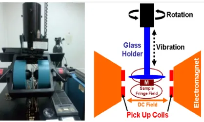
Overall, assays were performed involving magnetic nanoparticles (MNP) and cells labelled with MNP. These assays were performed with a platform mentioned above, containing a permanent magnet assembled with the chip which was integrated with an electronic platform from INESC-ID, allowing signal acquisition from magnetized nanoparticles.
In a very preliminary stage, magnetic particles between 2800 nm and 50 nm were tested flowing through a 100 µm wide, 50 µm high microchannel, with speeds around 50 µL/min being detected. Bipolar and unipolar signals with average amplitude of 15 µV – ~250 µV were observed corresponding to magnetic events. A home-made program to count magnetic events was developed in Matlab®.
In particular it is presented an example for the validation of the platform as a magnetic counter that identifies and quantifies
Staphylococcus spp. cells magnetically labelled with 50nm particles in a milk sample. In assays using 500 µL of milk
sample, cells were detected with signal amplitude of 30 µV – ~200 µV.
Key-words:
cytometers, magnetoresistive sensors, permanente magnet, magnetic nanoparticles, Staphylococcus spp..XI
Contents
Resumo ... V Abstract ... IX List of figures ... XIII List of Tables ... XX List of Acronyms ... XXI
Introduction ... 23
1.1 Objectives ... 24
1.2 Thesis Structure ... 24
1.3 State of the Art ... 25
Theoretical Background ... 31
2.1 Magnetic Dipoles ... 31
2.1.1 Magnetic Materials Properties ...31
2.2 Giant Magneto-Resistance (GMR) and Spin Valve (SV) sensors ... 35
2.3 Biosensors ... 39
Materials and Methods ... 41
3.1 Spin Valve Chip Design ... 41
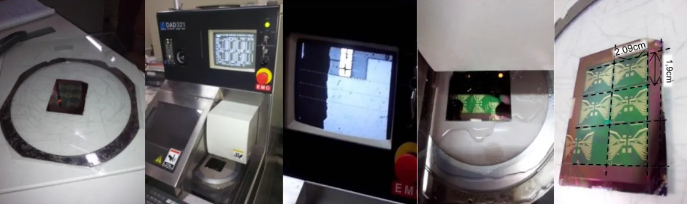
3.2 Microfabrication ... 42
3.3. Electrical Transport Characterization of SV sensors ... 48
3.4 Microfluidic system: PDMS channels and permanent bonding ... 50
3.5 Wirebonding and Encapsulation... 51
3.6 Magnetic Labelling and detection ... 52
3.6.1 Magnetization Method ...53
3.6.2 Detection Scheme ...53
3.7 Characterization of Magnetic Nanoparticles ... 55
Biochip Platform ... 61
XII
4.1.1 Electrical Transport Characterization of SV sensors with the permanent magnet ... 62
4.2 Design and Development of the Second Platform ... 64
4.2.1 Electrical Transport Characterization of SV sensors with the permanent magnet ... 65
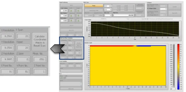
4.3 Development of a Magnetic Scanning Platform ... 66
4.3.1 Magnetic Scanning Analysis ... 69
4.3.2 Microfluidic Tests performed in the Platform with the permanent magnet ... 70
4.4 Second Spin Valve Chip Design ... 71
4.4.1 Chip Re-Design ... 71
4.4.1.1 Electrical Transport Characterization with the Permanent Magnet ... 72
Integration of the Biochip Platform with a portable electronic system ... 81
5.1 Electronic read-out of the sensors ... 81
5.2 Design and Development of the Third Platform ... 82
5.3. Experimental Results ... 83
5.3.1 Counting ... 84
5.3.2 Validation of micro-sized and nanometer-sized magnetic particles detection... 86
5.3.3 Detection of Biomolecular Recognition ... 95
Conclusions and Future work ... 101
Bibliography ... 103
A. Run Sheet: Magnetic Counter ... 111
B. Run Sheet: PDMS Microchannels ... 123
XIII
List of figures
Figure 1.1 Schematic representation of mastitis development in an infected udder. Environmental and contagious microorganisms invade the udder through the teat cistern. They multiply in the udder where they are attacked by neutrophils while damaging the epithelial cells lining the alveoli, with subsequent release of enzymes and anti-microbial components. The immune effector cells begin to combat the invading pathogens [1]. ...25 Figure 2.2 Representation of the magnetic moment associated with (a) an orbiting electron and (b) a spinning electron [5]. 31 Figure 2.3 Schematics of the gradual change in magnetic dipole orientation across a domain wall [5]. ...32 Figure 2.4 Schematic of the mutual alignment of atomic dipoles for a ferromagnetic material, which will exist even in the absence of an external magnetic field [5]. ...33 Figure 2.5 Representation of antiparallel alignment of atomic dipoles for antiferromagnetic manganese oxide [5]. ...33 Figure 2.6 Representation of domains in a ferromagnetic material. Arrows represent the atomic magnetic dipoles; the direction of alignment varies from one domain to another [5]...33 Figure 2.7 Exchange interaction between the antiferromagnetic and ferromagnetic layer. Top layer: Parallel alignment of the dipoles of the free pinned ferromagnetic layer. Bottom layer: Antiparallel alignment of the dipoles of the pinned ferromagnetic layer. ...34 Figure 2.8 Ferromagnetic material divides itself into magnetic domains to reduce the demagnetizing field therefore reducing the magnetostatic energy. Figure adapted from [30] ...35 Figure 2.9 Schematics of the SV sensor composed by a pinned layer and a free layer with parallel anisotropies [6]. ...35 Figure 2.10 Typical device structure: the two ferromagnetic layers separated by a nonmagnetic spacer. The arrows define the magnetization of each layer, upon the material acquires a shape. The antiferromagnetic layer (AFM) is introduced to fix the magnetization of the adjacent layer (pinned layer). ...36 Figure 2.11 a) Magnetostatic coupling between magnetic layers; b) Dipolar coupling between layers [21]. ...36 Figure 2.12 a) Transfer curve corresponding to parallel induced anisotropies, upon material deposition, showing that the magnetization reversal process along easy axis is predominantly domain wall motion; b) and c) Schematics of the effects of the material shape and dimensions in the crystalline anisotropy and shape anisotropy fields. The transfer curves show that the magnetization is a reversal process along the hard axis, which produces a coherent rotation of a domain wall motion. The PL crystalline anisotropy does not change his magnetization because it is fixed by AFM layer [6]. ...37 Figure 2.13 MR transfer curve principle. R(H) linear behaviour and typical magnetization orientations correspondence. The yellow arrows represent the free layer magnetization rotation and the blue arrows represent the pinned layer magnetization. ...38
XIV
Figure 2.14 Resistance vs. magnetic field transfer curve of a linear spin-valve at a given sense current. Red arrows
represent magnetization direction of PL and the yellow ones represent the magnetization direction of the FL. ... 39
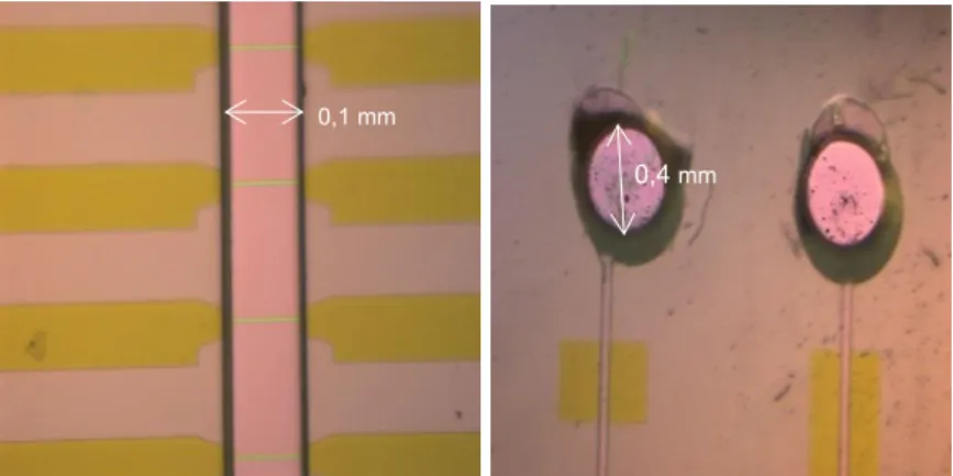
Figure 3.15 Design detailed of the biochip mask in AutoCad®: chip array of 28 SVs in red displayed vertically in the centre of the chip, the contact leads are presented in blue lines and the frame for electrical contact at the end of each contact leads displayed in green lines. ... 41
Figure 3.16 Schematics of one SV structure used in my thesis. ... 42
Figure 3.17 (A) SVG autonomous coating and development tracks system; (B) Direct Write Laser (DWL) system for lithography exposures; (C) AutoCad® Mask for first lithography: sensor’s definition. Chip with array of 28 SVs in red displayed vertically in the centre of the chip. ... 43
Figure 3.18 Ion beam system configured for the ion milling and O2 bonding mode. In this configuration only the assist gun is activated in order to etch the substrate surface. ... 44
Figure 3.19 Etching process: a) Patterning of the PR by photolithography b) Etching of the non-protected thin film layer c) sample after etch and resist strip. ... 44
Figure3.20 AutoCad® mask for second lithography: contact leads definition. The contact leads are presented in blue. ... 44
Figure 3.21 Thin film deposition process. ... 45
Figure 3.22 Photoresist and metal lift-off in wet bench. ... 45
Figure 3.23 Optical verification of Si3N4 deposition: passivation layer. ... 45
Figure 3.24 Design AutoCad® of the chip with the SV displayed in red. The frame for electrical contact at the end of each contact lead is displayed in green. ... 46
Figure 3.25 Reactive ion etching for pads opening. a) Visual and b) microscopic verification of defined SV, vias and contacts. ... 46
Figure 3.26 Sample was cut into individual dies. ... 46
Figure 3.27 a) Resist stripping; b) Microscope observation. ... 47
Figure 3.28 Annealing of each individualized chips. ... 47
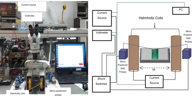
Figure 3.29 a) Transport Characterization setup; b) Schematic diagram of the setup employed for the electrical characterization. ... 48
Figure 3.30 Electrical Transport Characterization, MR curve of the Spin valve. ... 49
Figure 3.31 Top view of the microchannels in the AutoCad® mask and assembled mold and PMMA plates for PDMS casting. ... 50
Figure 3.32 Microscopic picture of the PDMS microchannel aligned with sensors on the chip. ... 50
XV
Figure 3.34 a) Wire bonding machine; b) Microscope picture of the connections between sensors contacts and the copper contacts of the PCB; c) PCB with mounted and bonded biochip. ...51 Figure 3.35 superparamagnetic particles behaviour in the presence and absence to an external magnetic field. ...52 Figure 3.36 Schematics of MR sensor detection of magnetically labeled targets flowing above the sensor for perpendicular magnetzation A [10] and B [4]; Perpendicular magnetization gives origin to an average field with a bipolar configuration C. 54 Figure 3.37 Picture of the VSM system used at INESC-MN and schematic illustration of the pick up coils and quartz rod. ...56 Figure 3.38 Magnetic properties of magnetic beads, measured by VSM. a) Magnetic moment per 50nm particle. b) Magnetic moment per 2800nm particles. ...56 Figure 3.39 Simulation of the average of the magnetic field sensed by the sensor relative to position of the MNP over distance from the sensor. a) Magnetic field along x-direction of a 50nm particle at height z=1 and z=10; b) Magnetic field along x-direction of a 2800nm particle at height=1 and 10; c) Magnetic field along x-direction of a 50nm particle at different heights. These simulations were permormed using the MAPLESOFT 12 software. ...58 Figure 3.40 Detection schematics (not to scale) of a magnetically particle, parallel magnetized, flowing over a SV sensor. The graphic represents an example of a simulated signal for 5 µm diameter cells, labelled with N= 2880 nanoparticles, parallel magnetized, at different heights [ 3, 7, 10] µm l. Adapted from [10]. ...58 Figure 4.41 Detailed design of the biochip mask in AutoCad®: chip array of 28 SVs is displayed in red, vertically in the centre of the chip, the contact leads are presented in blue lines and the frame for electrical contact at the end of each contact leads displayed in green lines. ...61 Figure 4.42 a) Assembly of the Biochip with the magnet, that is glue on the PCB; b) Schematics of the platform, showing the thicknesses of the different components of the platform. ...61 Figure 4.43 MR curve of the SV a) without a permanent magnet below; b) assembled with the permanent magnet. ...62 Figure 4.44 Schematics of the impact of the sensor response of each magnetic field component, set by magnet position transfer curves [4]. ...63 Figure 4.45 Schematics of the free and pinned layer magnetizations in the absence of a magnetic field. ...63 Figure 4.46 a) AutoCad® design of the support platform; b) Schematics of the full assembled integrated platform; c) Fotography of the full assembled integrated platform with the biochip and the squared permanent magnet. ...64 Figure 4.47 MR curve of the SV a) without a permanent magnet below; b) assembled with the permanent magnet at 0,5 cm distance; c) assembled with the permanent magnet at 1 cm distance; d) assembled with the permanent magnet at 2 cm distance. ...65 Figure 4.48 Magnetic scanning platform. ...66 Figure 4.49 Schematics of an Hall Effect sensor principle [16]. ...67
XVI
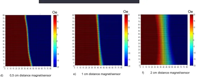
Figure 4.50 Use of an Hall Effect sensor for permanent magnet measurement of: perpendicular and in-plane magnetic fields. The sensor passes above the permanent magnet and their lines of force act on the chip. ... 68
Figure 4.51 Schematics of the measurements of the permanent magnet. ... 68 Figure 4.52 LabView softawe developed for the permanent magnet scanning masurements. ... 69 Figure 4.53 Perpendicular ( a), b), c) ) and Longitudinal ( d), e), f) ) magnetic field scan results from the surface of the permanent magnet at different heights from the sensor. The resolution used in the scanning was 0.25 mm, so the dimensions of the magnet are showen in the graphics multiplicated to 0.25. ... 69 Figure 4.54 a) Dynabeads® M-280; Photography of: b) experimental setup; c) a section of the microchannel where a sample that contains water, magnetic particles and blue dye can be observed under a microscope using a magnification of 20x. ... 71 Figure 4.55 Top view of the biochip in the AutoCad® mask (A); Four arrays of spin valve sensors (B); One group of spin valve sensors (C). ... 72 Figure 4.56 MR curve of the SVs a) without a permanent magnet below; b) assembled with the permanent magnet at 1 cm distance; c) assembled with the permanent magnet at 2 cm distance. ... 72 Figure 4.57 Representation of the impact of positioning of magnet in sensors transfer curve parameters: A. Magnetoresistivity; B. Effective coupling field; C. Coercive field. ... 75 Figure 4.58 Schematics of a non perpendicular orientation between the F layer and P layer, which promote discontinuities in sensor magnetic response to an external magnetic field. F: Free; P: Pinned (P). ... 75 Figure 4.59 Schematics of the linearization of the sensor due to the presence of the permanent magnet. F: Free; P: Pinned (P). ... 76 Figure 4.60 (A) AutoCAD® design of the chip; (B) Array of SVs is zoomed showing the location of SVs number 15 and 23, refered below. ... 76 Figure 4.61 Tranfer curves of SV number 15 and 23 obtained when: a) there is no permanent magnet below; b) a permanent magnet is placed at 1 cm from the SVs; c) a permanent magnet is placed at 2cm below the SVs. The graphics show the influences on the tranfer curves caused by the permnent magnet presence below the sensors. ... 77 Figure 4.62 Tranfer curves of four SVs, localized in each one of microchanels, obtained when: a) there is no permanent magnet below; b) a permanent magnet is placed at 1 cm from the SVs; c) a permanent magnet is placed at 2cm below the SVs. The graphics show the influences on the tranfer curves caused by the permanent magnet presence below the sensors. ... 78 Figure 5.63 Setup used in the experiments: 1) Biochip platform; 2) batteries for power supply and portability; 3) acquisition board, which encrypts the data collected from sensors; 4) Digital to analogue converter (DAC), it is responsible for the data conversion and transition to the device for user interface (computer); 5) Syringe pump to impose flowrates; 6) User interface (computer)... 81
XVII
Figure 5.64 AutoCad® PCB design. ...82 Figure 5.65 Assembly of the platform with the SV chip and permanent magnet to PCBs and data acquisition electronic platform. ...83 Figure 5.66 Acquisition setup assembly. ...83 Figure 5.67 Statistical analysis of the noise measured from a sample containing non-magnetic material. The standard deviation is ~ 3.86 µV and for counting calculations (in this case) was considered to be between ± 4σ. So, in this case, the threshold should be 4 x (±3.86 x10-06) = ± 1.54x10-05 V. ...85
Figure 5.68 Example of data acquired (104 points) by one sensor when a buffer with magnetic particles flow inside the
microchannel. The counting peaks software counts just the peaks above the threshold defined by the noise to the noise background. ...85 Figure 5.69 Data acquired by the SV 7: a) No sample inside the microchannel; b) When a buffer pass through the microchannel, corresponding to the noise background. ...86 Figure 5.70 Statistical analysis of the noise measured from a sample containing non-magnetic material. The standard deviation is ~ 8 µV and for counting calculations (in this case – SV 7) was considered to be between ± 5σ. The threshold should be 5 x (±8.02 x10-06) = ± 4.05x10-05 V. ...87
Figure 5.71 Representative figure of three single peak detection response of one sensor to one trial of 30 second run of the sample M-280 Streptavidin magnetic particles. The peak amplitude values are displayed in µV. ...87 Figure 5.72 Number of peaks counted and their amplitude. ...88 Figure 5.73 Data acquired by the SV 3: a) No sample inside the microchannel; b) When a buffer passes through the microchannel, corresponding to the noise background. ...88 Figure 5.74 Statistical analysis of the noise measured from a sample containing non-magnetic material. The standard deviation is ~ 2 µV and for counting calculations (in this case – SV 3) was considered to be between ± 5σ. The threshold should be 5 x (±2.26 x10-06) = ± 1.13x10-05 V. ...89
Figure 5.75 Representative figure of two single peak detection response of SV 3 to one trial of 30 second run of the sample 250nm magnetic particles. The peak amplitude values are displayed in µV...89 Figure 5.76 Number of peaks counted and their amplitude. ...90 Figure 5.77 Data acquired by the SV 10: a) No sample inside the microchannel; b) When a buffer flow through the microchannel, corresponding to the noise background. ...90 Figure 5.78 Statistical analysis of the noise measured from a sample containing non-magnetic material. The standard deviation is ~ 2 µV and for counting calculations (in this case – SV 10) was considered to be between ± 4σ. The threshold should be 4 x (±3.86 x10-06) = ± 1.54x10-05 V. ...91
XVIII
Figure 5.79 Representative figure of peak detection response of one sensor to one trial of 30 second run of the sample 130
nm magnetic particles. A zoom is applied to four single peaks. The peak amplitude values are displayed in µV. ... 91
Figure 5.80 Number of counted peaks and their amplitude. ... 92
Figure 5.81 Data acquired by the SV 12: a) No sample inside the microchannel; b) When a buffer flow through the microchannel, corresponding to the noise background. ... 92
Figure 5.82 Statistical analysis of the noise measured from a sample containing non-magnetic material. The standard deviation is ~ 0.5 µV and for counting calculations (in this case – SV 12) was considered to be between ± 4σ. The threshold should be 4 x (±3.86 x10-06) = ± 1.54x10-05 V. ... 92
Figure 5.83 Representative figure of non-peak detection response of one sensor to one trial of the sample 80 nm magnetic particles. A zoom of the date showed that values are above the defined threshold. ... 93
Figure 5.84 Data acquired by the SV 8: a) No sample inside the microchannel; b) When a buffer flow through the microchannel, corresponding to the noise background. ... 93
Figure 5.85 Statistical analysis of the noise measured from a sample containing non-magnetic material. The standard deviation is ~ 0.3 µV and for counting calculations (in this case – SV 8) was considered to be between ± 4σ. The threshold should be 4 x (±3.86 x10-06) = ± 1.54x10-05 V. ... 94
Figure 5.86 Representative figure of non-peak detection response of one sensor to one trial of 30 second run of the sample 50 nm magnetic particles. ... 94
Figure 87 Schematics of immuno-magnetic functionalization of cells. a) 50 nm Superparamagnetic particle; b) Protein A; c) anti-staphylococci spp. monoclonal antibody; d) Staphylococcus Cell; e) Staphylococci immunogenic protein. ... 95
Figure 5.88 Acquired signal: a) sensor base noise level ; b) raw milk blank sample; c) raw milk with functionalized nanoparticles (control sample). ... 96
Figure 5.89 Statistical analysis of the noise measured from a sample containing non-magnetic material. The standard deviation is ~13 µV and for counting calculations (in this case – SV 4) was considered to be between ± 6σ. The threshold should be 6 x (±5.16 x10-06) = ± 3.1x10-05 V. ... 97
Figure 5.90 Raw milk sample with Staphylococcus cells. The peak amplitude values are displayed in µV. ... 98
Figure 5.91 Number of peak counts of the sample measured and the amplitude. ... 98
Figure A92 Spin Valve layers. ... 111
Figure A93 Overall Process of the third step. ... 112
Figure A94 AutoCad® Mask for first lithography: sensor’s definition. Chip with array of 28 SVs in red displayed vertically in the centre of the chip. ... 113
Figure A95 Schematics of physical etching. ... 114
XIX
Figure A97 Second lithography process. ... 115
Figure A98 AutoCad® mask for second lithography: contact leads definition. The contact leads are presented in blue. .... 116
Figure A99 Schematics of Thin film deposition process. ... 118
Figure A100 Photoresist and metal litf-off process. ... 118
Figure A101 Schematics of Si3N4 deposition: passivation layer. ... 119
Figure A102 Third lithography process. ... 119
Figure A103 Design AutoCad® of the chip with the SV displayed in red. The frame for electrical contact at the end of each contact lead is displayed in green. ... 120
Figure A104 Schematics of reactive ion etching for pads opening. ... 121
Figure A105 Sample was cut into individual dies. ... 122
XX
List of Tables
Table 1.1 Diagnostic overview of bovine mastitis [1, 2]. ... 27
Table 3.2 Simulations of the average magnetic field sensed by the sensor relative to position of the MNP at a certain height (z). ... 57
Table 3.3 Simulations of the voltage output measured by the sensor relative to position of the MNP at a certain height (z). 57 Table 4.4 Important parameters taken from SVs transport characterization ... 65
Table 4.5 Important parameters taken from the MR curve of the SVs without a permanent magnet below. ... 73
Table 4.6 Important parameters taken the MR curve of the SVs with a permanent magnet below at 1 cm. ... 73
Table 4.7 Important parameters taken the MR curve of the SVs with a permanent magnet below at 2 cm. ... 73
Table 4.8 Values obtain from the equation above, showing the impact of the contribution of the permanent magnet field components in saturation field sensors transfer curve. ... 77
Table 4.9 Values obtained from the equation above, showing the impact of the positioning of the magnet below the sensors due to the contribution of the permanent magnet field components in saturation field sensors transfer curve. ... 79
Table 5.10 Statistical analysis of the noise measured from a sample containing non-magnetic material. ... 85
Table 5.11 Statistical parameters of the SV 7 signal without sample flowing inside ... 87
Table 5.12 Statistical parameters of the SV 3 signal without sample flowing inside ... 89
Table 5.13 Statistical parameters of the SV 10 signal without sample ... 91
Table 5.14 Statistical parameters of the SV 12 signal without sample flowing... 93
Table 5.15 Statistical parameters of the SV 8 signal without sample ... 94
Table 5.16 Statistical parameters of the SV 4 signal without sample flowing inside microchannel, from a milk sample, milk sample with functionalized MNPs and a milk sample with bacteria’s labelled with functionalized MNPs. ... 97
XXI
List of Acronyms
Ab AFM CIISA DC DWL ELISA FL FM GMR GPIB IBD IBM INESC-MN INESC-ID MNPs MR PBS PCB PDMS PECVD PL PMMA POC PR SCCs SV UHV II UV - O VSM Antibody AntiferromagneticCentro de Investigação Interdisciplinar em Sanidade Animal Direct Current
Direct Write Laser
Enzyme-Linked Immunoabsorbent Asay Free Layer
Ferromagnetic
Giant Magnetoresistance General Purpose Interface Bus Ion Beam Deposition
International Business Machines Corporation
Instituto de Engenharia de Sistemas e Computadores – Microsistemas e Nanotecnologias Instituto de Engenharia de Sistemas e Computadores – Investigação e Desenvolvimento Magnetic Nanoparticles
Magnetoresistance Phosphate Buffer Saline Printed Circuit Board Poly(dimethylsiloxane)
Plasma Enhanced Chemical Vapour Deposition Pinned Layer
Poly-methyl-methacrylate Point-of-Care
Photoresist Somatic cell counts Spin Valve
Ultra-High Vacuum II Ultraviolet and Ozone
23
Chapter 1
Introduction
Regarding milk production, bovine mastitis continues to be an economically important disease being difficult to estimate the losses associated with clinical mastitis, which arises from the costs of treatment, culling, death and decreased milk production.
Beside financial implications of mastitis, the importance of this disease in public health should not be overlooked. The extensive use of antibiotics in its treatment and control has possible implications for human health through the increased risk of antibiotic resistance strains of emerging bacteria that may then enter in the food chain. Diagnostic methods have been developed to check the quality of the milk through detection of mammary gland inflammation and diagnosis of the infection and its pathogens, but these methods have their limitations and there is a need of new, rapid, sensitive and reliable assays.
Since 2000, INESC-MN has pioneered research and development on spintronic based lab on chip platforms for biomolecular recognition events. These are recognized by integrated spintronics transducers: Spin Valves or Magnetic Tunnel Junctions.
At INESC-MN, Point-of-Care platforms have already been designed, fabricated and tested for: DNA based assays (gene expression chips-CF mutation detection), proteins and cell assays (Salmonella, E. coli) and lateral immune assays (antibiotics in meat). The control electronics acquisition setup was also developed leading to two prototypes: one for static biomolecular recognition, where probes are immobilized over sensor sited and the signal is recorded as labelled targets hybridized with the probes, and another that is a dynamic cell counter for labelled cells as they pass over sensors, while flowing inside microfluidic channels.
This thesis focuses on an optimization of the dynamic cell counter prototype for the identification and quantification of bacteria, Staphylococci.
Hopefully, this device will contribute as an integrated part of a magnetoresistive Point-of-Care system, serving as an efficient tool.
Counting Analysis
Milk sample Microfluidic
channel
Spin Valve
24
1.1 Objectives
The present work follows the research done at INESC-MN on a biosensor system based on antibody recognition of mastitis pathogen, which uses a permanent magnet as magnetization source. This avoids the need of an external power source, enabling a more compact device and portable tests, which provides additional flexibility on their employment and also lowers the production costs of tests.
The detection scheme used in this platform relies on magnetoresistive (MR) sensor’s sensitivity to count cells in flow, detecting bacterial cell events as these pass over the sensor. However, the external permanent magnet, which is placed below the sensor, creates a strong field gradient that causes changes in sensor’s behaviour and also magnetic nanoparticles agglomeration at microchannels. A more homogeneous magnetic field needs to be implemented in order to minimize this effect.
The main goal of this thesis relies on the optimization of the integration of the chip that contains an array of sensors, with a permanent magnet, making possible to have more than one sensor functional to be used in measurements of four different samples simultaneously. In this way, this thesis supports a device capable of performing the counts of bacteria cells in an accurate, quantitative, easy and fast way.
To achieve these objectives there are some main tasks:
I. Fabrication of Spin Valve (SV) sensors and their assembly with a microfluidic module.
II. Biosensor system optimizations to allow the use of a permanent magnet as magnetization source without affecting the sensors, in order to be possible to use more than one sensor measuring at the same time.
III. Connection of the biosensor to an acquisition setup.
IV. Validation of the assembled device’s ability to detect different magnetic particles and, further on, magnetically labelled bacteria.
1.2 Thesis Structure
This thesis is organized as explained below.
After a brief introduction that includes a state of the art on systems for mastitis detection, chapter 2 includes a theoretical background. Chapter 3 is focused on the material and methods for the fabrication of the biochip, its assembly in the platform and the description of microfluidic system.
The experimental chapters are then divided into chapter 4 that comprises the integration of the biochip with permanent magnets, results and respective conclusions and chapter 5 which contains the integration of the
25
biochip platform, developed and fabricated (Chapter 3) at INESC-MN, with a portable electronic system developed in association with INESC-ID, assessing the detection of magnetic particles and cells in a Biochip. Finally, chapter 6 closes the project with general conclusions and future perspectives.
1.3 State of the Art
Bovine mastitis (mast = breast; it is = inflammation) is defined as an inflammation of the mammary gland. Organisms as diverse as bacteria, mycoplasmas, yeasts and algae have been implicated as causes of the disease. Fortunately, the vast majority of mastitis is of bacterial origin, being related with only five species of bacteria: Echerichia coli, Streptococcus uberis, Staphylococcus aureus, Streptococcus agalactiae and
Streptococcus dysgalactiae.
The potential spread of zoonotic organisms via milk, though it is rare in the era of pasteurisation, remains a risk especially in the niche markets of unpasteurised dairy products and during pasteurisation failures.
The traditional concept of environmental mastitis is that organisms live in the environment and contaminate the teats.
Invasion of the udder is considered to occur when the teat orifice is open. Usually, the teat canal is tightly closed by sphincter muscles, preventing the entrance of pathogens. However, when fluid accumulates within the mammary gland as parturition approaches, it results in an increased intramammary pressure and mammary gland becomes vulnerable due to dilatation of the teat canal leakage of mammary secretions. In addition, during the milking there is a distention of the teat canal and the sphincter requires ~2h to return back to the constricted position, Figure 1.1, [1].
Following rapid bacteria multiplication in the milk, an inflammatory response is mounted. The severity of the disease is then thought to be influenced in part by the speed of the immune response, in particular polymorphonuclear cell migration into the udder.
Figure 1.1 Schematic representation of mastitis development in an infected udder. Environmental and contagious microorganisms invade the udder
through the teat cistern. They multiply in the udder where they are attacked by neutrophils while damaging the epithelial cells lining the alveoli, with subsequent release of enzymes and anti-microbial components. The immune effector cells begin to combat the invading pathogens [1].
26
Early diagnosis is of the utmost importance due to the high costs of mastitis. Currently, milk quality payments are based on somatic cell counts (SCCs), and elevated levels result in reduced payments [1].
In Europe, elevated SCCs above 200 000 cells/mL are widely used as an indicator of mastitis and are determined using haemocytometers or cell counters [1]. Measurements of SCC lower than 1 x 10³
cells/mL indicates normal milk while during the infection it can rise to above 1 x 10⁶
27
Currently measurement of SCCs and alternative methods for detection of mastitis have been developed such as:
Table 1.1 Diagnostic overview of bovine mastitis [1, 2].
Advantages Disadvantages
California Mastitis Test
(CMT)
Simple cow-side indicator test for subclinical mastitis by somatic cell count estimation of milk. The measurement in milk samples uses a test reagent which
reacts with the DNA in those cells, forming a gel. The viscosity achieved by the aggregation of nucleic acids is proportional to the leukocyte number.
- Cost effective - Rapid - User friendly - Portable
- Results are difficult to interpret - Low sensitivity
Portacheck This method uses an esterase-catalysed enzymatic reaction to determine the SCC
in milk.
- Cost effective - Rapid - User friendly
- Low sensitivity at low SCCs
Fossomatic SCC
Fluorometric assay that uses ethidium bromide that penetrates and intercalate with the nuclear DNA and a fluorescent signal is generated and used to estimate the
SCC in milk. - Rapid - Expensive - Complex to use Delaval Cell Counter
This counter operates on the principle of optical fluorescence, where propidium iodide is used to stain nuclear DNA to estimate the SCC in milk.
- Rapid - Portable - Expensive R-mastitest (Electrical conductivity test)
This is an indirect test for cow’s mastitis diagnosis and as it measures the increase in conductance in milk caused by the elevation in levels of ions during
inflammation.
- Portable - Non-mastitis related variations
in Electrical conductivity can present problems in diagnosis.
pH test Colorimetric assay. The rise in milk pH, due to mastitis, is detected using
bromothymol blue
- Cost effective - Rapid - User friendly
28 In vitro culture
based diagnosis
Milk samples can be taken for bacterial, viral and fungal culture in a specific media and further microbiological/biochemical tests are used to identify different
microorganisms involved in mastitis cause.
- Identifies specific pathogens causing mastitis - A laboratory is needed to perform the tests - Time consuming
- Culture is capable of detecting only viable cells
PCR based diagnosis
Multiplex PCR: can identify multiple pathogens in a single reaction at the same time.
Real time PCR: Circulating miRNA:
- PCR based detection from mastitis milk samples are less time consuming - PCR assay is based on DNA and thus no
matter of live or dead organisms
- A laboratory is needed to perform the tests
- PCR detects lower number of organisms
- Costly instruments and consumables
Immune assay ELISA: enzyme-linked immunosorbent assay is a test that uses antibodies and
colour change to identify a substance.
- Rapid
- Antigens of very low or unknown concentration can be detected
- A laboratory is needed to perform the tests
- Only monoclonal antibodies can be used as matched pairs - Negative controls may indicate
positive results if blocking solution is ineffective.
Proteomics based detection
Proteomic tools as two-dimensional gel electrophoresis and mass spectroscopy helped to identify various proteins expressed during mastitis.
- It is the only technique that can be routinely applied for parallel quantitative expression profiling of complex protein mixtures such as whole cell and tissue lysates
- It is the most widely used method for efficiently separating proteins, their variants and modifications
- the complexity of biological structures and physiological processes
- Proteins expressed at low abundance may be missed -
Biosensors Biological sensors which use bio-receptors like antibody, nucleic acid, enzymes,
and produce a signal after combination with transducers.
- Rapid - Portable - User friendly - Cost effective
- Results are difficult to interpret - Low sensitivity
29
At present, control of the disease is centred on reducing environmental challenges around parturition and during lactation and ensuring strict hygiene both at and after milking. The biggest challenge facing the modern industries is the pressure to reduce the use of antibiotics in food producing animals, coupled with the dramatic increase in organic milk production in recent years [3].
For the past three decades, advances in sample pre-treatment, flow handling, precision technologies and bioinformatics have allowed the introduction of some sophisticated analytical tools in the cell/molecular biology areas, industrial bioprocesses, disease diagnostics, and so many other fields. In addition to detection and enumeration, some flow cytometers have the ability to sort cells at high speeds based on detected signals. Over the past years, the drawbacks of conventional flow cytometers have triggered efforts to take advantages of microfabrication and microfluidics technologies to achieve smaller, simple, low-cost instrumentation and enhanced portability for in-situ measurements.
The Lab-on-Chip approach has been making use of inexpensive polymers and detection techniques integrated with electronics, for example optical fibres, diode lasers, electrodes and magnetoresistive sensors. Some platforms present a static detection, where labels complementary to the target are immobilized on the sensors surface. However these platforms are limited by the sensors surface area and number of immobilized labels/targets.
This project addresses the optimization of permanent magnet integration on a biochip, which comprises MR sensors and microfluidics, as magnetic source for magnetic nanoparticles that flow inside microchannels. The ultimate goal is the to detect and count Staphylococci and Streptococci cells in milk samples in collaboration with a colleague at INESC-MN doing a PhD on veterinary and portable platforms for milk analysis.
31
Chapter 2
Theoretical Background
Magnetism is the phenomenon by which material assert an attractive or repulsive force or influence on other materials.
Iron, some steels and the mineral iodestone are examples of materials that exhibit magnetic properties. However all substances are influenced by the presence of a magnetic field.
2.1 Magnetic Dipoles
Magnetic forces are generated by moving electrically charged particles. Imaginary lines of force may be draw to indicate the direction of the force at positions in the vicinity of the field source.
Magnetic dipoles are found to exist in magnetic materials and can be compared to electric dipoles. Magnetic dipoles may be seen as small bar magnets composed of north and south poles instead of positive and negative electric charges. These dipoles are influenced by the magnetic field in a manner similar to the way in which electric dipoles are affected by electric fields.
2.1.1 Magnetic Materials Properties
Macroscopic magnetic properties of materials are a consequence of magnetic moments associated with individual electrons. Each electron in an atom has magnetic moments being originated from two sources:
I. Related to its orbital motion around the nucleus. An electron being a moving charge may be considered to be a small current loop that generates a very small magnetic field and has a magnetic moment along its axis of rotation, Figure 2.2a).
II. Related to its spinning movement around an axis. Spin magnetic moments may only be in an up direction or down direction, and thus each electron in an atom may be perceived as a small magnet having permanent orbital and spin magnetic moments, Figure 2.2b).
Figure 2.2 Representation of the magnetic moment associated with (a) an
32
In each individual atom, orbital moments of some electron pairs cancel each other. The net magnetic moment for an atom is just the sum of the magnetic moments (both orbital and spin contributions) of each of the constituent electrons.
For an atom which has completely filled electron shells or subshells, when all electrons are considered, there is a total cancellation of both orbital and spin moments. Thus, materials composed by atoms with completely filled electron shells are not capable of being permanently magnetized, such as the inert gases and some ionic materials.
All materials exhibit some type of magnetism, whose behaviour depends on the response of electron and atomic magnetic dipoles to the application of an external applied magnetic field. According to their magnetic properties, the materials can be classified into five distinct groups: diamagnetic materials, paramagnetic materials, ferromagnetic materials, antiferromagnetic materials and ferrimagnetic materials.
In this study it was used some of these materials, which are described below:
Paramagnetic material
The atoms of paramagnetic materials have a permanent magnet moment in absence of a magnetic field, due to the unpaired electrons on their partially filled shell, Figure 2.3. Since these atoms, as magnetic dipoles, poorly interact with each other they get random orientation due to thermal agitation. In the presence of an external magnetic field, the moments increasingly align with the field as the intensity of the field increases. Paramagnetic materials have positive and small susceptibility [5].
Ferromagnetic material
This material exhibits a large permanent magnetization even when a magnetic field is not present. The atoms of ferromagnetic materials have unpaired electrons, so the electron spins are not cancelled. Furthermore, coupling interactions cause spin magnetic moments of adjacent atoms to align with one another. When a magnetic field rises the individual moments tend to align with the field, Figure 2.4. The saturation magnetization (Ms) is achieved when all the magnetic dipoles are mutually align with the external field. Ferromagnetic materials have positive and large susceptibility [5].
Figure 2.3 Schematics of the gradual change in magnetic dipole
33
Antiferromagnetic material
In antiferromagnetic materials, the interaction between their atoms results in individual magnetic moments with antiparallel alignment, Figure 2.5. Manganese oxide (MnO) is an example of such material, having Mn2+
and O
2-ions. No net magnetic moment is associated with O2-,
since there is a total cancelation of both spin and orbital moments. However, Mn2+
ions have a net magnetic moment that is predominantly of spin origin and they are arrayed in the crystal structure such that the moments of adjacent ions are antiparallel. Since the opposing moments cancel one another with equal magnetic magnitude, the net magnetic moment in the absence of magnetic field is zero [5]. Antiferromagnetic materials have positive and small susceptibility.
Exchange energy
Any ferromagnetic or ferrimagnetic material is composed of small volume regions in which there are mutual alignments of all magnetic dipole moments in the same direction, Figure 2.6. Such region is called a domain, and each domain is magnetized to its saturation magnetization.
Figure 2.5 Representation of antiparallel
alignment of atomic dipoles for antiferromagnetic manganese oxide [5].
Figure 2.6 Representation of domains in a ferromagnetic material.
Arrows represent the atomic magnetic dipoles; the direction of alignment varies from one domain to another [5].
Figure 2.4 Schematic of the mutual alignment of atomic dipoles for a ferromagnetic material, which will exist even in the absence of an external magnetic field [5].
34
According to the theoretical model of atomic dipoles for ferromagnets, each permanent dipole interacts strongly with its nearest dipoles.
Dipoles are aligned in a parallel or antiparallel way depending if the material is ferromagnetic or antiferromagnetic, respectively. Exchange interaction between the antiferromagnetic and ferromagnetic layers determines the magnetization of the adjacent ferromagnetic layer, Figure 2.7.
In order to keep a minimum value of energy, the magnetic dipoles have a preference to remain aligned with each other.
Magnetocrystalline energy
Crystalline materials are magnetically anisotropic as the main crystallographic axis of the structure provides for a preferential direction for orientation of the dipoles . This direction is called easy direction.
In this way, the magnetocrystalline anisotropy energy, Ek, corresponds to the work that is necessary to rotate the
sample magnetization to a certain direction different of easy axis direction. This energy has a minimum value for an angle of zero between the magnetization and the easy axis, which means that when the magnetic field decreases to zero, the material will tend to align their dipole with easy axis.
Shape anisotropy
As mentioned above, crystalline materials have a preferential direction for orientation of the dipoles along the main crystallographic axis of the structure.
However, when a shape is given to the material, a magnetization is induced by reorientations of the dipoles in order to minimize energy and it is called demagnetizing field or self-demagnetizing field, Figure 2.8
Figure 2.7 Exchange interaction between the antiferromagnetic and ferromagnetic layer. Top layer: Parallel alignment of the dipoles of
35
2.2 Giant Magneto-Resistance (GMR) and Spin Valve (SV) sensors
A GMR structure is composed essentially by four thin films: a free layer (sensing layer) (FL), a conducting spacer, a pinned layer (PL) and an antiferromagnetic magnetic layer. The pinned, free and conducting layers are very thin, allowing the electrons to be frequently conducted back and forward the spacer. The magnetic orientation of the pinned layer is fixed and held in place by the adjacent antiferromagnetic layer. The magnetic orientation of the sensing layer changes in response to the magnetic field (H) [6,7].
The interaction among the layers normally aligns the magnetization of adjacent layers in opposite directions and electrons of both spins are scattered equally. If an external field is applied it aligns all the layers in one direction and it leads to a reduction of electrons scattering of one of the spins. As a consequence, the resistance of the sensor drops [7].
2.2.1.1 Macroscopic model for coherent rotation
Upon material deposition, both FL and PL have a configuration where their uniaxial induced anisotropy axes are parallel (parallel anisotropies), Figure 2.9.
For the linearization of magnetoresistive (MR) sensors with micrometric dimensions, is considered that layers have a magnetic single-domain so edge effects can be neglected. The magnetization of a single ferromagnetic layer, M, can be described as a single collective vector, whose magnitude (saturation magnetization - Ms)
𝑀𝐹𝐿
𝐻𝑑𝐹𝐿 𝐻𝑁 𝐻𝑘
Figure 2.9 Schematics of the SV sensor composed by a pinned layer and a free layer with parallel anisotropies [6].
𝐻𝑑𝑅𝑒𝑓
Figure 2.8 Ferromagnetic material divides itself into magnetic domains to reduce the demagnetizing field therefore reducing the magnetostatic energy. Figure adapted from [30]
36
remains constant and orientation may vary in space and time,. The total energy associated with sensing layer has some contributions [6]:
𝐄𝐅𝐥= 𝐄
𝐇+ 𝑬𝒅𝑭𝑳+ 𝐄𝐤+ 𝑬𝒅𝑷𝑳+ 𝐄𝐍 Equation 1
Where:
- EH is the Zeeman energy or external field energy.
- 𝐸𝑑𝐹𝐿 is the demagnetization field energy or shape anisotropy energy of the free layer. The demagnetization energy, Ed measures the interaction between the magnetic film and demagnetizing field. When the material acquires a shape, a magnetization - self-demagnetizing field - is induced by reorientation of the dipoles in order to minimize its energy, Figure 2.10.
- Ek is the crystalline anisotropy term. The minimum Ek is obtained when ∅ is 0º or 180º, i.e, when the
domains are orientated along the easy axis.
- 𝐸𝑑𝑃𝐿is the demagnetizing field energy of the pinned layer.
- ENis the Néel energy. The Neél coupling field (HN), induced by correlation between interface roughness
at the spacer interfaces with ferromagnetics. In spintronic multilayers, magnetostactic fields largely arise from roughness-induced surface poles. As device dimensions are reduced, the magnetic layers within stacks are more likely to become a single-domain, and then structural magnetostactic fields become more important, Figure 2.11.
Figure 2.10 Typical device structure: the two ferromagnetic layers separated by a nonmagnetic spacer. The arrows define the magnetization of each layer, upon the material acquires a shape. The antiferromagnetic layer (AFM) is introduced to fix the magnetization of the adjacent layer (pinned layer).
Figure 2.11 a) Magnetostatic coupling between magnetic layers; b) Dipolar coupling between layers [21].
37
To understand the conditions required for the linear behaviour of the MR device, Figure 2.12, one can consider the energy balance of the sensing layer with the following structure PL/Spacer/FL where the system is considered to be under the influence of an external field low than 500 Oe for the PL to have its magnetization fixed [6].
Figure 2.12a) represents the magnetization anisotropy, HK, for the FL defined in parallel orientation with respect to the PL. In this configuration, the SV shows a step response from a maximum high resistance state to low
resistance state, near the zero applied magnetic fields, reflecting the fact that the magnetization reversal process along easy axis is predominantly domain wall motion.
Figure 2.12b) shows schematics of the magnetization anisotropy of the FL defined in the transverse orientation with respect to the pinned layer due to the shape anisotropy effects. This allows the rotation of the magnetization of the FL when a magnetic field is applied, translating into a linear response of the SV between a high and low plateaus, reflecting the fact that the magnetization reversal process along the hard axis produces a coherent rotation instead of a domain wall motion. The uniaxial anisotropy can be obtained by applying a magnetic field during the film deposition or annealing process (Section 3). The origin of the induced anisotropy is the short range directional ordering, in which atomic pairs in a film tend to align with the local magnetization [6].
Applied Field (H) 1 2 3 H R 1 2 3 Hc R 1 2 3 H Hc FL PL HK 𝐻𝑑𝐹𝐿 HK c) R 1 2 3 H Hc ~ 0 FL PL HK HK b)
Figure 2.12 a) Transfer curve corresponding to parallel induced anisotropies, upon material deposition, showing that the magnetization reversal
process along easy axis is predominantly domain wall motion; b) and c) Schematics of the effects of the material shape and dimensions in the crystalline anisotropy and shape anisotropy fields. The transfer curves show that the magnetization is a reversal process along the hard axis, which produces a coherent rotation of a domain wall motion. The PL crystalline anisotropy does not change his magnetization because it is fixed by AFM layer [6]. FL PL a) HK HK HK HK 1 2 3 Applied Field (H) 𝐻𝑑𝐹𝐿 1 2 3 Applied Field (H)
38
Carefull patterning and dimensioning of the SV is needed to manipulate the demagnetizing field of the FL, HdFL,
Figure 2.12c).For the parallel anisotropy it is crucial that the FL induces a demagnetizing field along the easy axis direction, which is promoted by the shape anisotropy.
The easy axes for stable magnetization direction are 0 and π radians. If one cycle of magnetic field is applied in the perpendicular direction to the easy axis in ferromagnetic films, the magnetization direction changes from 0 to
𝜋
2radians as the magnetic field increases, and 𝜋
2to π radians as he magnetic field decreases, Figure 2.13.
When Hext -HdPL+HN < |Hk-NhMsFL|, two distinct situations can occur. If the induced anisotropy term is higher than
The magnetization direction of the PL can only be reversed at fields above the exchange bias field which can be as high as 500 Oe for pinned layers comprising a single ferromagnetic and anti-ferromagnetic layers.
2.2.1.2 Sensor Transfer Curve
The sensor behaviour is characterized by its transfer curve, which represents directly the output resistance dependence on field signal.
The name SV appears because if an external field is applied, this sensor acts as a valve for one of the electron spins. SV are sensitive not only the magnitude but also to the direction of the field in the plane [8].
A magnetoresistive device is a transducer which converts an external field into a resistance given a DC bias current supply.
The devices have a minimum (Rmin) and a maximum (Rmax) resistance plateau and the path from one level to the
other should to be linear, allowing them to work as magnetic field sensors, Figure 2.14. The magnitude of magnetoresistance effect is defined as follows:
Figure 2.13 MR transfer curve principle. R(H) linear behaviour and typical magnetization orientations correspondence. The yellow arrows represent the
free layer magnetization rotation and the blue arrows represent the pinned layer magnetization.
Free Layer Spacer Pinned Layer AFM Layer Substrate No external H field a External H field Free Layer Spacer Pinned Layer AFM Layer Substrate b External H field Free Layer Spacer Pinned Layer AFM Layer Substrate c
Strong external H field
Free Layer Spacer Pinned Layer AFM Layer Substrate d c R H b d a
39
𝐌𝐑(%) =𝐑𝐦𝐚𝐱−𝐑𝐦𝐢𝐧
𝐑𝐦𝐢𝐧 × 𝟏𝟎𝟎 Equation 2
The GMR materials typically have MR ratios about 10-50% [9].
Saturation fields define the ideal linear range of the device, where a dR variation corresponds to a single dH value. The key feature of a magnetic sensor response is its field sensitivity, which represents how the sensor is reactive to a field variation. It can be measured experimentally from the slope of the transfer curve.
The sharp magnetization reversal near zero magnetic field is due to the switching of the FL in the presence of its weak coupling to PL. The relative orientations of two magnetic layers were indicated by the pairs of arrows in each region of the MR curve, where the resistance is larger for antiparallel alignment of the two magnetic layers [9].
2.3 Biosensors
The ability of magnetoresistive sensors to detect weak magnetic fields is present in many different applications. New and promising areas are biomedicine and biotechnology. In the last decade, biomolecular recognition plays an important role in areas such as health care, pharmaceutical industry and environmental analysis.
The main idea behind magnetoresistive biochips is to provide a good alternative to the traditionally used fluorescent marker devices. These devices use an expensive optical or laser-based fluorescence scanning system to detect fluorescent labelled biomolecules that recognize a known biomolecule which is previously immobilized on the sensor surface.
Among the variety of affinity biosensor systems based on biomolecular recognition and labelling assays, magnetic labelling and detection is emerging as a promising new approach. In magnetic biochips, the fluorescent markers are replaced by nanoparticles, and a magnetic sensor detects the stray field produced by the label giving an electrical signal. Magnetic labels can be non-invasively detected by a wide range of methods, are physically and chemically stable, relatively inexpensive to produce, and can easily be made biocompatible.
α
-HSat HSat
RMax
RMin
Figure 2.14 Resistance vs. magnetic field transfer curve of a linear spin-valve at a given sense current. Red arrows represent magnetization
direction of PL and the yellow ones represent the magnetization direction of the FL.
S = MR
∆Hlinear
![Figure 3.36 Schematics of MR sensor detection of magnetically labeled targets flowing above the sensor for perpendicular magnetzation A [10] and B [4];](https://thumb-eu.123doks.com/thumbv2/123dok_br/15448449.1026657/54.892.95.798.445.1012/figure-schematics-detection-magnetically-labeled-targets-perpendicular-magnetzation.webp)