Spectral and Homogenization Problems
Rita Alexandra Gon¸calves Ferreira
Dissertation for the Degree of Doctor of Philosophy
in Mathematics
Supervisors:
Professor Irene Fonseca (MCS/CMU)
Professor M. Lu´ısa Mascarenhas (FCT/UNL)
Spectral and Homogenization Problems
Rita Alexandra Gon¸calves Ferreira
Dissertation for the Degree of Doctor of Philosophy
in Mathematics
Supervisors:
Professor Irene Fonseca (MCS/CMU)
Professor M. Lu´ısa Mascarenhas (FCT/UNL)
Acknowledgments
I want to express my deep gratitude to my supervisors, Professor Irene Fonseca and Professor Lu´ısa Mascarenhas, for their availability, for their constant support and encouragement, and for having shared with me their vast scientific and human knowledge.
I also want to express my sincere appreciation to Professor Giovanni Leoni as his door was always open for any question and support.
I also would like to thank the members of my thesis committee, Professor Ana Barroso, Professor Irene Fonseca, Professor Diogo Gomes, Professor David Kinderlehrer, Professor Giovanni Leoni, and Professor Lu´ısa Mascarenhas, for their comments and suggestions on the first draft of my thesis. I am very thankful to the CMU | Portugal Ph.D. Program for having provided me with myriad opportunities in the realm of academia, as I have been exposed to several research groups, and have been given the opportunity to interchange ideas with people from different cultures and having different backgrounds, and also to present my research work at several scientific meetings.
I am extremely grateful to the Department of Mathematical Sciences at Carnegie Mellon University and to the Department of Mathematics at Faculdade de Ciˆencias e Tecnologia da Universidade Nova de Lisboa for their hospitality.
Quero exprimir o meu profundo agradecimento `a minha fam´ılia, em especial aos meus pais, pela infinita paciˆencia, pelo permanente apoio e pelo imenso carinho que sempre me dispensaram. A special Thank You! to my friends for always being there for me. Foremost I thank Pittsburgh for introducing me to my better half. Thanks Ricardo for your unconditional love and support.
Abstract
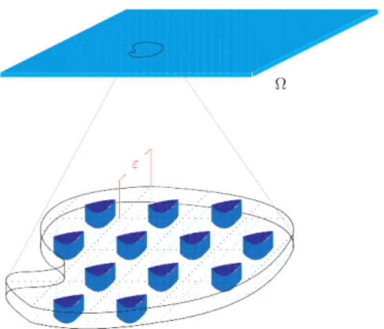
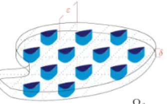
In this dissertation we will address two types of homogenization problems. The first one is a spectral problem in the realm of lower dimensional theories, whose physical motivation is the study of waves propagation in a domain of very small thickness and where it is introduced a very thin net of heterogeneities. Precisely, we consider an elliptic operator with"-periodic coefficients and the corresponding Dirichlet spectral problem in a three-dimensional bounded domain of small thickness . We study the asymptotic behavior of the spectrum as"and tend to zero. This asymptotic behavior depends crucially on whether"and are of the same order ( ⇡"), or"is of order smaller than that of ( ="⌧, ⌧ <1), or" is of order greater than that of ( = "⌧, ⌧ > 1). We consider all three
cases.
The second problem concerns the study of multiscale homogenization problems with linear growth, aimed at the identification of effective energies for composite materials in the presence of fracture or cracks. Precisely, we characterize (n+1)-scale limit pairs (u, U) of sequences{(u"LN
bΩ, Du"bΩ)}">0⇢
M(Ω;Rd) ⇥ M(Ω;Rd⇥N) whenever {u"}">0 is a bounded sequence in BV(Ω;Rd). Using this characterization, we study the asymptotic behavior of periodically oscillating functionals with linear growth, defined in the spaceBV of functions of bounded variation and described byn2Nmicroscales.
Resumo
Nesta disserta¸c˜ao ser˜ao tratados dois problemas no ˆambito da teoria da homogeneiza¸c˜ao. O primeiro refere-se a um problema espectral no dom´ınio das teorias de baixa dimens˜ao, que tem como motiva¸c˜ao o estudo de propaga¸c˜ao de ondas em dom´ınios de pequena espessura e onde ´e introduzida uma fina rede de heterogeneidades. Mais precisamente, consideramos um problema espectral definido num dom´ınio tridimensional de espessura , com condi¸c˜oes de Dirichlet nulas, associado a um operador el´ıptico com coeficientes"-peri´odicos. Apresentamos o comportamento assimpt´otico do espectro quando"e tendem para zero, distinguindo trˆes casos: o caso em que a frequˆencia das oscila¸c˜oes e a espessura do dom´ınio s˜ao da mesma ordem de grandeza ("⇡ ), o caso em que a frequˆencia das oscila¸c˜oes ´e muito maior do que a espessura do dom´ınio ( = "⌧, ⌧ < 1) e, finalmente, o caso em que a espessura do
dom´ınio ´e muito menor do que a frequˆencia das oscila¸c˜oes ( ="⌧, ⌧ >1).
O segundo problema aqui tratado reporta-se ao estudo de problemas de homogeneiza¸c˜ao caracterizados por m´ultiplas escalas microsc´opicas e condi¸c˜oes de crescimento lineares, que tˆem em vista a identifica¸c˜ao da energia efectiva de comp´ositos com fracturas ou rachas. Mais precisamente, caracterizamos os pares limite a (n + 1)-escalas (u, U) de sucess˜oes {(u"LN
bΩ, Du"bΩ)}">0 ⇢
M(Ω;Rd)⇥ M(Ω;Rd⇥N) em que {u"}">0 ´e limitada. Usando esta caracteriza¸c˜ao, estudamos o comportamento assimpt´otico de funcionais periodicamente oscilantes com condi¸c˜oes de crescimento lineares, definidos no espa¸coBV das fun¸c˜oes de varia¸c˜ao limitada e caracterizados porn2Nescalas microsc´opicas.
Notation and List of Symbols
Symbol/Expression
N,Z, andR: set of natural, integer, and real numbers N0 : {0} [N
R+ : set of positive real numbers Rm: m-dimensional Euclidean space
[x] andhxi (x2Rm) : integer and fractional parts of xcomponentwise, respectively ⇠·⇣ or (⇠|⇣) (⇠, ⇣2Rm) : Pm
i=1⇠i⇣i
Zm: (z1,· · ·, zm) : zi2Zfor alli2 {1,· · ·, m} Md⇥N : space ofd⇥N-dimensional matrices A⇠⇣ (A2MN⇥N,⌘, ⇣2RN) : (A⇠|⇣)
⇠⌦⇣ (⇠2Rd,⇣2RN) : (⇠
i⇣j)16i6m,16j6d2Md⇥N
Rd⇥N : space ofd⇥N-dimensional matrices identified withRdN ⇠:⇣ (⇠, ⇣2Rd⇥N) : Pd
i=1
PN
j=1⇠ij⇣ij
|⇠| (⇠2Rd⇥N) : p⇠:⇠
(· | ·) or (· | ·)H : inner product in a Hilbert spaceH
k · kork · kX : norm in a Banach spaceX
h·,·i: duality pairing
ij : Kronecker symbol
∆ : Laplacian
r: gradient div : divergence
ri or @x@i : first order partial derivative with respect to the variablexi
∆ior @
2
@x2
i : second order partial derivative with respect to the variablexi Y (reference cell) : (0,1)N or [0,1]N
Yi withi2N: copy ofY
subscript # : Y1⇥· · ·⇥Yn-periodic functions (or measures) w.r.t.the variables (y1,· · ·, yn)
@Ω (Ω⇢RN) : boundary of Ω
Ω0⇢⇢Ω (Ω⇢RN) : Ω0 compact with Ω0 ⇢Ω
Ω domain (Ω⇢RN) : Ω open and connected
suppf, Lipf : support and Lipschitz constant, respectively, of a functionf
f⇤,f⇤⇤ : polar (or conjugate) and bipolar functions, respectively, of a functionf
Cf,Qf : convex and quasiconvex envelopes, respectively, of a functionf C(Ω),C(Ω;Rd) : space of real- andRd-valued continuous functions in Ω, respectively
Cc(Ω),Cc(Ω;Rd) : space of functions inC(Ω) andC(Ω;Rd), respectively, with compact support
C0(Ω),C0(Ω;Rd) : closure ofCc(Ω) andCc(Ω;Rd), respectively, w.r.t.the supremum norm C#(Y1⇥ · · · ⇥Yn) : Y1⇥ · · · ⇥Yn-periodic, real-valued continuous functions inRN
C#(Y1⇥ · · · ⇥Yn;Rd) : Y1⇥ · · · ⇥Yn-periodic,Rd-valued continuous functions inRN
f 2Cc(Ω;C#(Y1⇥ · · · ⇥Yn)) : for all x 2 Ω, f(x,·) 2 C#(Y1 ⇥ · · · ⇥Yn) and for all y1, ..., yn 2 RN,
f(·, y1, . . . , yn)2Cc(Ω)
f 2Cc(Ω;C#(Y1⇥ · · · ⇥Yn;Rd)) : for all x2 Ω, f(x,·) 2C#(Y1⇥ · · · ⇥Yn;Rd) and for ally1, ..., yn 2 RN,
f(·, y1, . . . , yn)2Cc(Ω;Rd)
C0(Ω;C#(Y1⇥ · · · ⇥Yn)) : closure ofCc(Ω;C#(Y1⇥ · · · ⇥Yn)) w.r.t.the supremum norm
C0(Ω;C#(Y1⇥ · · · ⇥Yn;Rd)) : closure ofCc(Ω;C#(Y1⇥ · · · ⇥Yn;Rd)) w.r.t.the supremum norm
Ck(Ω),Ck(Ω;Rd) : space of all functions in C(Ω) andC(Ω;Rd), respectively, whoseith-partial derivatives are continuous functions in Ω for all i 2 {1,· · ·, k}; the spacesCk
c(Ω;Rd),C0k(Ω;Rd),C#k(Y1⇥ · · · ⇥Yn;Rd),Cck(Ω;C#k(Y1⇥
· · · ⇥Yn;Rd)), andC0k(Ω;C#k(Y1⇥ · · · ⇥Yn;Rd)), with the co-domain
omitted ifd= 1, are defined in an obvious way
C1(Ω),C1(Ω;Rd) : space of all functions in Ck(Ω) andCk(Ω;Rd), respectively, for all k 2 N; the spacesC#1(Y1⇥· · · ⇥Yn;Rm),Cc1(Ω;C#1(Y1⇥· · · ⇥Yn;Rd)), and
C1
0 (Ω;C#1(Y1⇥ · · · ⇥Yn;Rd)), with the co-domain omitted ifd= 1,
are defined in an obvious way Lp(Ω),Lp(Ω;Rd) : usual Lebesgue spaces
W1,p(Ω),W1,p(Ω;Rd) : usual Sobolev spaces
BV(Ω),BV(Ω;Rd) : space of functions of bounded variation *,*? : weak and weak-?convergence, respectively
B(X) : -algebra of the Borel subsets of a topological spaceX
M(X;Z) (Z Banach space) : space ofZ-valued Radon measures
Ld : d-dimensional Lebesgue measure
a.e. inRd : everywhere inRd except in a set of zerod-dimensional Lebesgue measure M(⇣, ⌘,Ω) : set of allN⇥N real matricesA= (aij)16i,j6N 2[L1(Ω)]N⇥N bounded and
MS(⇣, ⌘,Ω) : set of all N⇥N real, symmetric matricesA= (aij)16i,j6N 2[L1(Ω)]N⇥N
bounded and coercive a.e. in Ω
D(A), R(A), N(A), G(A) : domain, range, kernel, and graph, respectively, of an operatorA
Table of Contents
Acknowledgments v
Abstract vii
Resumo ix
Notation and List of Symbols xi
Chapter 1. Introduction 1
1.1 Spectral Analysis in a Thin Domain with Periodically Oscillating Characteristics 4 1.2 Reiterated Homogenization inBV via Multiscale Convergence 6
Chapter 2. Preliminaries 11
2.1 Measure Theory 11
2.1.1 Positive Measures. . . .11
2.1.2 Measurable Functions. . . .13
2.1.3 Decomposition and Differentiation of Measures. . . .15
2.1.4 Signed Measures. . . .16
2.1.5 Product Measures. . . .18
2.1.6 Space of Radon Measures as a Dual Space. . . .19
2.1.7 Disintegration of Measures. . . .21
2.1.8 Reshetnyak’s Continuity and Lower Semicontinuity Results. . . .21
2.2 Lebesgue and Sobolev Spaces 22 2.2.1 Lebesgue Spaces. . . .22
2.2.2 Sobolev Spaces. . . .24
2.3 Integration with Respect to Functions of Bounded Variation-Valued Radon Measures 27 2.3.1 Space of Functions of Bounded Variation. . . .27
2.3.2 Integration with respect toBV#(Y;Rd)-valued Radon measures. . . .29
2.4 Unbounded Linear Operators in Hilbert Spaces: Spectral Theory 38 2.4.1 Quadratic Forms and Associated Unbounded Linear Operators. . . .41
2.4.2 The Case of Elliptic Partial Differential Operators. . . .42
2.5 Γ-Convergence andG-Convergence 44 2.5.1 Γ-Convergence. . . .44
2.5.2 G-Convergence. . . .48
Chapter 3. Spectral Analysis in a Thin and Periodically Oscillating Medium 51
3.1 Main Results 51
3.2 Preliminary Results 57
3.3 Proof of Theorem 3.1.1 ("⇡ ) 60
3.4 Proof of Theorem 3.1.2 ("⌧ ) 63
3.5 Proof of Theorems 3.1.4 and 3.1.7 (" ) 66
Chapter 4. Multiscale Convergence of Sequences of Radon Measures 79
4.1 Main Results 81
4.2 Multiscale Convergence inBV 83
Chapter 5. Reiterated Homogenization in BVvia Multiscale Convergence 113
5.1 Main Results 116
5.2 Proof of Theorem 5.1.3 122
5.3 Proof of Corollary 5.1.4 144
Chapter 6. Future Research Projects 149
Chapter 1
Introduction
This dissertation is devoted to the study of mathematical problems within the framework of homogenization theory, which addresses the description of the macroscopic or effective behavior of a microscopically heterogeneous system. There are multiple applications in the fields of physics, mechanics and engineering sciences, from which we emphasize problems aimed at the modeling of composites, stratified or porous media, finely damaged materials, or materials with many holes or cracks.
From the mathematical point of view, homogenization is often associated to the study of the asymptotic behavior of oscillating partial differential equations, or of minimization problems yielding from certain oscillating functionals, depending on one or more small-scale parameters. Several approaches have been proposed to handle this type of problems, such as the method of asymptotic expansions (see the books of Bensoussan, Lions and Papanicolaou [13], Jikov, Kozlov and Ole˘ınik [53], Bakhvalov and Panasenko [12], and Sanchez-Palencia [69]) and methods using the concepts of G-convergence due to Spagnolo (see Spagnolo [71] and De Giorgi and Spagnolo [35]),H-convergence due to Murat and Tartar (see Murat and Tartar [63], Tartar [73] and Murat [62]), Γ-convergence due to De Giorgi (See De Giorgi and Dal Maso [36] and De Giorgi and Letta [37]), and two-scale convergence due to Nguetseng (see Nguetseng [64]), further developed by Allaire [1] and Allaire and Briane [2]. For a comprehensive introduction to the theory of homogenization and for an overview of the different homogenization methods, we refer to the book of Cioranescu and Donato [28].
As a simple illustration of a homogenization problem, we briefly describe the problem regarding the study of the thermal conductivity of a periodic composite material. Composites are structures constituted by two or more finely mixed materials that, depending on the performance we are looking for, in general exhibit a better behavior than the average of its components, and for this reason they may have an impact in industrial applications. Loosely speaking, the smaller the heterogeneities, the better the mixture, which then seems homogeneous (see Fig. 1.0.1).
by
k"(x) :=k
⇣x " ⌘
,
where" >0 is a small parameter, andk is the Y-periodic function, beingY := [0,1]3 the reference cell1.1, defined for all y
2Y by
k(y) := ⇢
k1 ify2Y1, k2 ify2Y\Y1, whereY1 is a measurable subset ofY.
Fig. 1.0.1. Microscopically heterogeneous material
Note that
Ω1:=✓ [
z2Z3
"(z+Y1) ◆
\Ω and Ω2:=✓ [
z2Z3
"(z+Y\Y1) ◆
\Ω.
Assuming without loss of generality that the temperature on the surface@Ω of the body is zero and representing byf the heat source, then the temperatureu"=u"(x) at each pointx2Ω satisfies the
Dirichlet problem ⇢
div(k"ru") =f in Ω,
u"= 0 on@Ω.
(1.0.1) We observe that two scales characterize problem (1.0.1): the macroscopic one, x, which indicates the position in Ω, and the microscopic or fast-oscillating scale, x
", which assigns the position in the
reference cell, in the sense that there exists a uniquey2Y such that x
" =y+z for somez2Z
3. It is commonly agreed in the engineer and physics communities that the bigger is the ratio between the size of the body and the size of each of its separated components, that is, the smaller " is, the more stable are the physical properties (in this case, the heat transfer) of the mixture. Moreover, the global or effective behavior of the mixture generally differs from the average of its components. Heuristically, we seek to replace the heterogeneous material by a “fictitious” homogeneous material whose global characteristics are dictated by the effective properties. From the mathematical point of view, this reduces to the study of problem (1.0.1) in the limit as" !0+. Precisely, we want to investigate whether{u"}">0converges is some sense to some functionu0as"!0+, and, if so, we aim 1.1 For simplicity, we take here as reference cell the unit cube inR3, but we could have taken any bounded interval inR3,
at describing the limit problem of (1.0.1) that admitsu0 as solution. Under some mild hypotheses onf (see, for example, Cioranescu and Donato [28] for the details), the answer to these questions is affirmative: {u"}">0 converges weakly in H01(Ω), as " ! 0+, to a function u0, solution of the homogenizedDirichlet problem ⇢
div(Ahru) =f in Ω,
u= 0 on@Ω, (1.0.2)
whereAh:= (ah
ij)16i,j632M3⇥3is the constant matrix whose coefficients are given by ahij :=
Z
Y
k(y)⇣ ij @wj
@yi
⌘
dy, i, j2 {1,2,3}, where ij is the Kronecker symbol, andwj is the solution of thecell problem
8 > > < > > :
div(krwj) = @k
@yj
inY , wj Y-periodic,
Z
Y
wj(y) dy= 0.
(1.0.3)
The matrix Ah encodes the overall characteristics of the original mixture, and since it cannot be
written in the form aI, with a > 0 and I the identity matrix, we conclude that the homogeneous limit material is not isotropic. We also observe that the considerations above are still valid in any dimensionN 2N(and not justN = 3).
In this work we will sometimes adopt the variational point of view, i.e., instead of looking for solutions of boundary problems of the type (1.0.1) we will be interested in solutions of minimization problems associated with the energy functional corresponding to the physical system under study. For instance, in the case of problem (1.0.1), we would be led to the study of the minimization problem
min ⇢ Z
Ω
k"(x)|ru(x)|2dx 2
Z
Ω
f(x)u(x) dx: u2H01(Ω) . These minimization problems often assume the general form
min ⇢ Z
Ω
f"(x, Du(x)) dx: u2 A ,
whereAis the class of admissibleu’s. In the limit as"!0+ we expect a minimizationhomogenized
problem of the form
min
⇢ Z
Ω
fhom(Du(x)) dx: u2 A ,
wherefhom plays the role of the matrixAh in (1.0.2), and it is given byasymptotic homogenization
formulasorcell problem formulas, which correspond to the variational formulation of the cell problems (1.0.3).
1.1. Spectral Analysis in a Thin Domain with Periodically Oscillating Characteristics.
Within the framework of quantum mechanics, Schr¨odinger’s equation for the time-independent wave function associated to a particle in a three-dimensional space is given by:
¯
h
2m∆ +V =E ,
where ¯h :=h/2⇡, h being Plank’s constant, m is the mass of the particle, ∆ is the usual Laplace’s operator,V is the potential energy andE is the energy of the system with wave function . When we consider the particle to be confined to a certain domain Ω ⇢ R3, but otherwise free, precisely,
when the potential function is of the formV(x) := 0 if x2Ω, and V(x) := +1if x62Ω, then the problem of finding the spacial wave function and the energy levelsEreduces to solving the following eigenvalue problem for the Laplace’s operator:
⇢
∆v= v in Ω,
v= 0 on@Ω,
where, using standard mathematical notations, we identified ⌘ v and ⌘ 2m
¯
h E. In the joint
works with Mascarenhas [45] and with Mascarenhas and Piatnitski [46], we addressed this eigenvalue problem in the case in which the domain has a very small thickness and the material presents very small "-periodic heterogeneities. We proved that the energy levels depend strongly on both small parameters and"and on their ratio.
Precisely, let", >0 be small parameters, and consider the thin domain Ω :=!⇥ I, where!⇢R2
is a bounded domain, andI:= ( 1/2,1/2). Our goal is to study the asymptotic behavior as"!0+
and !0+ of the spectral problem
⇢
div(A"rv") = "v" a.e. in Ω ,
v" 2H1 0(Ω ),
(1.1.1)
whereA"(¯x) :=A(x"¯), ¯x2R2, withA= (aij)16i,j632[L1(R2)]3⇥3a real, symmetric andY-periodic
matrix, whereY := (0,1)2, satisfying appropriate boundedness and coercivity hypotheses. We assume
further thata↵3= 0 a.e. inY,↵2 {1,2}. We refer to Chapter 3 for the details.
The spectrum " of problem (1.1.1) is discrete and can be written as " := { ",i 2 R+: i 2 N},
where 0< ",i 6 ",i+1 for alli2N, and
",i !+1as i!+1. For fixed">0, as the thickness
of the domain goes to zero ( ! 0+) all the eigenvalues go to infinity. For fixed > 0, a classical
result in the theory of homogenization asserts that as"!0+ the eigenvalues converge to eigenvalues
associated with the corresponding homogenized problem of (1.1.1). As we mentioned before, in the case in which the small parameters"and converge to zero simultaneously, the asymptotic behavior of the spectrum " depends crucially on whether " and are of the same order (" ⇡ ), or" is of order smaller than that of (" ⌧ ), or" is of order greater than that of (" ). The results corresponding to the cases" ⇡ and "⌧ were announced in Ferreira and Mascarenhas [45]. In Ferreira, Mascarenhas and Piatnitski [46] detailed proofs of the statements formulated in Ferreira and Mascarenhas [45] were provided, and the case" was studied. Our main tools are Γ-convergence and asymptotic expansion techniques.
operator convergence have been introduced in Ole˘ınik, Shamaev and Yosifian [65] and Attouch [8]. Other homogenization approaches in spectral problems and related topics have been proposed by Allaire and Conca [3], Allaire and Malige [4]. The homogenization of singularly perturbed operators has been considered in Kozlov and Piatnitski [56], [57] and some other works. The novelty in the homogenization spectral problem treated here is its study in the realm of lower dimensional theories. We refer to Bouchitt´e, Mascarenhas and Trabucho [19], Gaudiello and Sili [50], Krejˇciˇr´ık [59], and to the references therein, for other spectral problems within lower dimensional theories.
A brief description of the case " ⇡ . Let ",k be akth eigenvalue associated with problem
(1.1.1) for =". Then (see Theorem 3.1.1)
",k= µ0
"2 +⌫",k,
whereµ0>0 is the first eigenvalue associated with a certain bidimensional periodic spectral problem
with nonzero potential. Moreover,⌫",k!⌫k as"!0+, with⌫k aktheigenvalue associated with the
bidimensional homogenized spectral problem in the cross section!
⇢
div( ¯Bhr¯') =⌫' a.e. in!,
'2H1 0(!),
(1.1.2)
where ¯Bh is a certain 2⇥2 constant matrix. Loosely speaking, the term µ0
"2 provides information on
how the eigenvalues ",k diverge, and also on the precise shift of the spectrum in order to retain the
macroscopic behavior of the physical problem under study, which is given by the limit problem (1.1.2). As expected this is a two-dimensional problem of the same type of the original three-dimensional one, but with constant coefficients. Note that ",k µ"20 k2N={⌫",k}k2N is the spectrum of the shifted operator div(A"r) µ"20I with zero Dirichlet boundary conditions, whereI represents the identity
operator.
The asymptotic behavior of the eigenfunctions associated with ",kwill also be provided. We refer to
Chapter 3 for the details.
A brief description of the case "⌧ . Assume thata↵ are uniformly Lipschitz continuous in
Y. Let ",kbe aktheigenvalue associated with problem (1.1.1) for ="⌧, with some⌧ 2(0,1), and
leti2Nbe such that i 1
i <⌧6 i+1i . Then (see Theorem 3.1.2)
",k= i
X
j=0 %j
"⌧(2j+2) 2j +⇢ ⌧ "+⌫",k,
where%0=⇡2
R
Y a33(¯y) d¯y >0, and forj2N,%jare well-determined constants. Furthermore,⇢⌧" !0
as "! 0+, ⌫
",k ! ⌫k as " ! 0+, with ⌫k akth eigenvalue associated with a certain bidimensional
homogenized spectral problem in the cross section !, of the same type as (1.1.2). Here, the sum
Pi j=0
%j
"⌧(2j+2) 2j plays the role of
µ0
"2 in the above case " ⇡ . The term ⇢⌧", which is innocuous in
the limit as it converges to zero, is related to this sum and we may think of it as a remainder. The asymptotic behavior of the eigenfunctions associated with ",kwill also be provided.
A brief description of the case " . i) This case is considerable more difficult to handle
than the previous ones, and it depends strongly on the behavior of the potentiala33. An interesting
case of composites). In that direction new hypotheses on a33 are introduced: Assume thata↵ are
smooth functions and that there exists an open and smooth subdomainQofY,Q⇢⇢Y, such that
a33 coincides with its minimum, amin, in Q and is a smooth function strictly greater thanamin in Y\Q. Let ",1be the first eigenvalue of problem (1.1.1) with ="⌧ for some⌧ 2(1,+1). Then (see
Theorem 3.1.4)
",1=
amin⇡2 "2⌧ +
⌫0 "2 +"
⌧ 3µ
1+· · ·+"k(⌧ 1) 2µk+⇢⌧"+⌫",⌧1,
wherekis the first integer greater or equal than 2/(⌧ 1),⌫0>0 is the first eigenvalue associated with
a certain bidimensional spectral problem onQ, andµi,i2 {1,· · ·, k}, are well-determined constants, |⇢⌧"|6C"(k+12)⌧ (k+52) !0 as" !0+, for some constant C independent of", and ⌫⌧
",1 vanishes as "!0+. In this case, the limit problem degenerates.
ii) Finally, under quite more general hypotheses than those above, we are able to characterize the limit spectrum in the sense of Kuratowsky: Assume thata33 attains a minimum value,amin, at some
¯
y02R2such thata↵ anda33are continuous in some neighborhood of ¯y0. Then (see Theorem 3.1.7)
lim
"!0+ "
2⌧
" =⇥amin⇡2,+1⇤, (1.1.3)
where "represents the spectrum of problem (3.1.2) with ="⌧ for some⌧2(1,+1), and the limit
in (1.1.3) is to be understood in the sense of Kuratowsky, that is,⇥amin⇡2,+1⇤is the set of all cluster
points of sequences{ "}">0, "2"2⌧ ".
1.2. Reiterated Homogenization in BV via Multiscale Convergence.
Within the framework of nonlinear elasticity, the elastic energy associated with an N-dimensional composite materials is of the form Z
Ω
f"(x,ru(x)) dx,
where Ω⇢RNdenotes the reference configuration,u: Ω!Rd is the deformation of the body, andf"
stands for the elastic stored density energy. We will assume thatf"satisfies linear growth conditions,
which is the natural setting for composite materials in the presence of fractures or cracks. In order to allow for jump-type discontinuities, we consider the space of admissible deformations to be the space
BV(Ω;Rd) of functions of bounded variation. In the presence of n microscales, or fast-oscillating
variables, we seek to characterize the asymptotic behavior as"!0+of energy functionals of the form
F"(u) :=
Z
Ω
f⇣ x
%1(")
,· · ·, x
%n(")
,ru(x)⌘dx+
Z
Ω
f1⇣ x
%1(")
,· · ·, x
%n(")
, dD
su
dkDsuk(x)
⌘
dkDsuk(x)
(1.2.1) foru2BV(Ω;Rd) withDu=ruLN
bΩ+Dsuthe Lebesgue decomposition ofDu with respect toLNbΩ,
where
f1(y1,· · ·, yn,⇠) := lim sup
t!+1
f(y1,· · ·, yn, t⇠)
t
is the recession function of a certain functionf :RnN⇥Rd⇥N !R, separately periodic in the firstn
variables and satisfying linear growth conditions, and%1, ...,%n are positive functions in (0,1) such
that for alli2 {1,· · ·, n}and for allj2 {2,· · ·, n},
lim
"!0+%i(") = 0, "lim!0+
%j(")
In the context of multiscale composites, the functions%1, ...,%nstand for thelength scalesorscales of oscillation. The second condition in (1.2.2) is known as a separation of scales hypothesis. A simple example of such functions%i is the case in which%i(") :="i,i2 {1,· · ·, n}.
We observe that for fixed " > 0, and under some hypotheses on f, the functional in (1.2.1) is the relaxed functional inBV(Ω;Rd) of
u7!
Z
Ω
f⇣ x
%1(")
,· · ·, x
%n(")
,ru(x)⌘dx
with respect to theL1(Ω;Rd) topology (see Fonseca and M¨uller [49]).
We now briefly describe the methodology adopted to carry out the aforementioned asymptotic characterization. In a joint work with Fonseca [43] we generalized the notion of two-scale convergence for sequences of Radon measures with finite total variation obtained in Amar [5] to the case of multiple periodic length scales of oscillations. The main result in Ferreira and Fonseca [43] concerns the characterization of the multiple-scale limit of{(u"LN
bΩ, Du"bΩ)}">0⇢ M(Ω;Rd)⇥ M(Ω;Rd⇥N)
whenever{u"}">0 is a bounded sequence inBV(Ω;Rd). Using this characterization and the periodic
unfolding method (see, for example, Cioranescu, Damlamian and De Arcangelis [26] and Fonseca and Kr¨omer [47]), in a subsequent joint work with Fonseca [44] we treated multiscale homogenized problems in the spaceBV of functions of bounded variation of the form (1.2.1). In the case of one microscale we recovered Amar’s result [5] under more general conditions, as well as Bouchitt´e’s result [16] and De Arcangelis and Gargiulo’s result [34]; for two or more microscales the results we obtained are new.
Precisely, let Ω ⇢ RN be an open set and let Y := (0,1)N. For i 2 N, Yi is a copy of Y. We
use the subscript # to represent Y1⇥ · · · ⇥Yn-periodic functions (or measures) with respect to
the variables (y1,· · ·, yn). We say that a sequence {µ"}">0 ⇢ M(Ω;Rm) of Radon measures with
finite total variation in Ω, (n+ 1)-scale converges to a Radon measure with finite total variation µ02 C0(Ω;C#(Y1⇥· · ·⇥Yn;Rm)) 0 ' My#(Ω⇥Y1⇥· · ·⇥Yn;Rm) in the product spaceΩ⇥Y1⇥· · ·⇥Yn, if for all'2C0(Ω;C#(Y1⇥ · · · ⇥Yn;Rm)) we have
lim "!0+
Z
Ω '
✓
x, x
%1(")
,· · ·, x
%n(")
◆
·dµ"(x) =
Z
Ω⇥Y1⇥···⇥Yn
'(x, y1,· · ·, yn)·dµ0(x, y1,· · ·, yn),
in which case we writeµ"(n+1)"-sc*µ0.
This notion of convergence is justified by a compactness result, which asserts that every bounded sequence in M(Ω;Rm) admits a (n + 1)-scale converging subsequence (see Theorem 4.1.3). Furthermore, the usual weak-?limit in M(Ω;Rm) is the projection on Ωof the (n+ 1)-scale limit, so that the latter captures more information on the oscillatory behavior of a bounded sequence in
M(Ω;Rm) than the former. This leads us to study the asymptotic behavior with respect to the (n+ 1)-scale convergence of first order derivatives functionals with linear growth of the form (1.2.1).
In that direction, the first step is the characterization of the (n+ 1)-scale limit associated with u"LN
bΩ, Du"bΩ "⇢ M(Ω;Rd)⇥ M(Ω;Rd⇥N),{u"}">0 being a bounded sequence inBV(Ω;Rd).
This was established in Ferreira and Fonseca [44] and may be summarized as follows (see Chapter 4 for the details). Assume that the length scales%1, ...,%n are, in addition, well separated (c.f. Allaire and Briane [2]), i.e., there existsm2Nsuch that for alli2 {2,· · ·, n}, we have
lim "!0+
✓
%i(")
%i 1(")
◆m 1
Then, up to a not relabeled subsequence,
u"LNbΩ(n+1)"-sc* ⌧u,
where⌧u2 My#(Ω⇥Y1⇥ · · · ⇥Yn;Rd) is a certain measure only depending onu, and Du"(n+1)"-sc* u,µ1,···,µn,
where u,µ1,···,µn 2 My#(Ω⇥Y1⇥ · · · ⇥Yn;R
d⇥N) is a certain measure depending on u and on n measures µi 2 M?(Ω⇥Y1⇥ · · · ⇥Yi 1;BV#(Yi;Rd)), i.e., measures µi 2 M(Ω⇥Y1⇥ · · · ⇥
Yi 1;BV#(Yi;Rd)) for which there exists a measure i2 My#(Ω⇥Y1⇥ · · · ⇥Yi;Rd⇥N) such that for
allB2 B(Ω⇥Y1⇥ · · ·Yi 1),E2 B(Yi), we have
Dyi(µi(B)) (E) = i(B⇥E).
The measures ⌧u and u,µ1,···,µn admit an explicit characterization, whose proof is not a simple
generalization of the casen= 1 treated in Amar [5]. In fact, considerable modifications are required whenn>2, similar to those in Allaire and Briane [2] in the Sobolev setting. Moreover, we found out that fully developing the underlying measure-theoretical background was not straightforward. Using the main results in Ferreira and Fonseca [43], in Ferreira and Fonseca [44] we characterized and related the functionals
Fsc(u,µ1,· · ·,µn) := infnlim inf
"!0+ F"(u") : u"2BV(Ω;
Rd), Du"(n+1)-sc
" * u,µ1,...,µn
o
and
Fhom(u) := infnlim inf
"!0+ F"(u") : u"2BV(Ω;
Rd), u"*? "uweakly-?inBV(Ω;Rd)o
foru2BV(Ω;Rd) andµi2 M?(Ω⇥Y1⇥ · · · ⇥Yi 1;BV#(Yi;Rd)),i2 {1,· · ·, n}, where F" is given
by (1.2.1).
Precisely, under certain hypotheses on the function f (see Chapter 5 for the details), for all (u,µ1,· · ·,µn)2BV(Ω;Rd)⇥ M
?(Ω;BV#(Y1;Rd))⇥ · · · ⇥ M?(Ω⇥Y1⇥ · · · ⇥Yn 1;BV#(Yn;Rd))
we have that (see Theorem 5.1.3)
Fsc(u,µ1,· · ·,µn) =
Z
Ω⇥Y1⇥···⇥Yn
f⇣y1,· · ·, yn,
d ac u,µ1,...,µn
dL(n+1)N (x, y1,· · ·, yn)
⌘
dxdy1· · ·dyn
+
Z
Ω⇥Y1⇥···⇥Yn
f1⇣y1,· · ·, yn,
d s
u,µ1,...,µn dk s
u,µ1,...,µnk
(x, y1,· · ·, yn)
⌘
dk s
u,µ1,...,µnk(x, y1,· · ·, yn).
(1.2.3) Moreover, for allu2BV(Ω;Rd),
Fhom(u) = inf
µ12M?(Ω;BV#(Y1;Rd)),...,
µn2M?(Ω⇥Y1⇥···⇥Yn 1;BV#(Yn;Rd))
Fsc(u,µ1,· · ·,µn)
=
Z
Ω
fhom(ru(x)) dx+
Z
Ω
(fhom)1
⇣ dDsu
dkDsuk(x)
⌘
dkDsuk(x),
(1.2.4)
wherefhom is given by a cell problem formula (see (5.1.4)).
[44] was proving a similar result without assuming coercivity, or boundedness from below, off. Such weak hypotheses are often useful to deal with degenerate media.
The main ingredients we will use to establish (1.2.3) and (1.2.4) are the unfolding operator (see Cioranescu, Damlamian and De Arcangelis [25], Cioranescu, Damlamian and Griso [27]; see also Fonseca and Kr¨omer [47]) and Reshetnyak’s continuity- and lower semicontinuity-type results. The approach via the unfolding operator, in connection with the notion of two-scale convergence and in the framework of homogenization problems, sometimes referred as periodic unfolding method, has already been adopted by other authors in the Sobolev setting (see, for example, Cioranescu, Damlamian and De Arcangelis [25], Cioranescu, Damlamian and De Arcangelis [26], Fonseca and Kr¨omer [47]).
This dissertation is organized as follows. In Chapter 2, we collect the basic notations and background results that are used in the subsequent chapters. In Chapter 3, we prove the results announced in Section 1.1 above concerning the asymptotic behavior as " ! 0+ and
! 0+ of the spectrum
of an elliptic operator with"-periodic coefficients in a three-dimensional bounded domain of small thickness . The aim of Chapter 4 is to prove the characterization of (n+ 1)-scale limit pairs (u, U) of sequences {(u"LNbΩ, Du"bΩ)}">0 ⇢ M(Ω;Rd)⇥ M(Ω;Rd⇥N) whenever {u"}">0 is a bounded
sequence in BV(Ω;Rd) referred in the Section 1.2. Finally, in Chapter 5, we treat multiple-scale
Chapter 2
Preliminaries
The aim of this chapter is to provide a survey of the concepts and known results used throughout this dissertation. At the beginning of each section we will give references where proofs of the results therein and further considerations on the corresponding topic may be found.
2.1. Measure Theory.
In this section we briefly overview properties of measures. We refer to the books Fonseca and Leoni [48], Rudin [68], Evans and Gariepy [40], Ambrosio, Fusco and Pallara [7], and to the references therein.
2.1.1. Positive Measures
Definition 2.1.1.( -algebra, measurable space, measurable set) LetX be a nonempty set. We say that a collectionM⇢ 2X is a -algebra (in X) if ; 2 M, X\E 2 Mwhenever E 2 M, and M is
closed under countable unions. IfM⇢2Xis a -algebra, we call the pair(X,M)a measurable space,
and a setE⇢X is said to be measurable ifE2M.
Definition 2.1.2.(Borel -algebra, Borel set)LetX be a topological space. The smallest -algebra inX that contains all open subsets ofX is called the Borel -algebra (inX) and is represented by
B(X). A setE2 B(X)is said to be a Borel set.
Definition 2.1.3.(Positive measure, measure space)Let(X,M)be a measurable space. We say that
a set mapµ:M![0,+1]is a positive measure onMifµ(;) = 0and µis countably additive, i.e.,
µ
✓+[1
j=1
Ej
◆
=
+1
X
j=1
µ(Ej) (2.1.1)
whenever{Ej}j2Nis a countable collection of mutually disjoint measurable sets. The triple(X,M, µ)
is called a measure space.
Definition 2.1.4.(Restriction of a measure)Let(X,M, µ)be a measure space and letE2M. The
measureµbE:M![0,+1]defined by
Definition 2.1.5.( -finite set, -finite and finite measures)Let (X,M, µ)be a measure space. A
setE2Mis said to have -finite µmeasure if it can be written as a countable union of measurable
sets of finiteµmeasure. In the case in which X has -finiteµmeasure we say that µis -finite. If µ(X)<+1we say thatµis finite.
The next result concerns monotone convergence properties of measures.
Proposition 2.1.6.Let(X,M, µ)be a measure space. If{Ej}j2N⇢Mis an nondecreasing sequence,
then
µ
✓+[1
j=1
Ej
◆
= lim
j!+1µ(Ej). If{Ej}j2N⇢Mis an nonincreasing sequence withµ(E1)<+1, then
µ
✓+\1
j=1
Ej
◆
= lim
j!+1µ(Ej).
Definition 2.1.7. (Borel, Borel regular and Radon measures; inner and outer regular sets) Let
(X,M, µ)be a measure space, withX a topological space. We say that
(i) µis a Borel measure ifB(X)⇢M;
(ii) µis a Borel regular measure if it is a Borel measure and for every setE2Mthere exists a set
F 2 B(X)such thatF E andµ(E) =µ(F);
(iii) µis a Radon measure if it is a Borel measure satisfying the following conditions:
(a) µ(K)<+1for every compact setK⇢X,
(b) every open setA⇢X is inner regular, i.eµ(A) = sup{µ(K) : K⇢A, K compact}, (c) every setE2Mis outer regular, i.eµ(E) = inf{µ(A) : A E, Aopen}.
Definition 2.1.8. (Support of a Borel measure) Let (X,M, µ) be a measure space, with X a
topological space andµa Borel measure. The support of µis the set
suppµ:= x2X: µ(O)>0for every open neighborhoodOofx .
Definition 2.1.9.(Negligible set) Let(X,M, µ)be a measure space. We say that a set M ⇢X is
µ-negligible if there is a measurable setE 2M such thatE M and µ(E) = 0. A property P(x)
depending onx2X is said to holdµ-almost everywhere inX (in short, to holdµ-a.e. inX or to hold forµ-a.e. x2X)2.1 if the set
{x2X: P(x)does not hold}isµ-negligible.
In applications it is often very important to guarantee that subsets of sets of zero measure are still measurable.
Definition 2.1.10.(Complete measure)Let(X,M, µ)be a measure space. We say thatµis complete
if given any setE2Mwithµ(E) = 0, then every subset ofE belongs toM.
2.1 Ifµis thel-dimensional Lebesgue measureLl,l2N, then its dependence is often omitted, and we simply writea.e. in
It is always possible to complete a measure. Precisely,
Proposition 2.1.11.Let(X,M, µ)be a measure space and letMcbe the collection of all setsE⇢X
for which there existF, G2Mwith F ⇢E ⇢Gand such thatµ(G\F) = 0. Define µc(E) :=µ(F).
ThenMc is a -algebra that containsM and µc : Mc ![0,+1] is a complete measure, which are
called theµcompletion ofMand the completion ofµ, respectively.
One of the most important examples of completion of a measure is the completion of the Lebesgue measure on the Borel -algebra.
Notation 2.1.12. Letl 2N. We will represent byLl both thel-dimensional Lebesgue measure on the Borel -algebra and its completion.
2.1.2. Measurable Functions
Definition 2.1.13. (Measurable and Borel functions) Let (X,M) and (Z,N) be two measurable
spaces. We say that a functionu:X !Z is measurable ifu 1(F)
2Mfor allF 2N. In the case in
whichX andZ are topological spaces,M=B(X)andN=B(Z)we say thatuis a Borel function.
Remark 2.1.14.IfX andZ are topological spaces, a functionu:X !Z is Borel if, and only if, for every open setA⇢Z we haveu 1(A)2 B(X).
We now extend the notion of measurability to functions defined everywhere except in a set of zero measure.
Definition 2.1.15.(Generalization of the notion of measurable function)Let(X,M, µ)and(Z,N)
be a measure and a measurable space, respectively, and letE2Mbe such thatµ(X\E) = 0. We say
thatu:E!Z is measurable overX ifu 1(F)2Mfor allF 2N.
Remark 2.1.16. Let (X,M, µ) be a measure space and let u : E ! [ 1,+1] be a measurable
function overX, where E 2 M is such that µ(X\E) = 0. Then the functionu˜ : X ![ 1,+1]
defined by
˜
u(x) :=
⇢
u(x) ifx2E,
0 ifx2X\E,
is measurable andRXu˜dµ=REudµ, where R dµis the usual Lebesgue integral with respect to the measureµ.
Definition 2.1.17.(Simple function) Let (X,M) be a measurable space. We say that a function
s:X !Ris a simple function if it is measurable and if it takes finitely many values. Ifc1, ...,cmare the distinct values ofs, then we write
s=
m
X
i=1
ci Ei,
where Ei is the characteristic function of the measurable setEi:=s
1(
{ci}).
Theorem 2.1.18.Let(X,M)be a measurable space andu:X![ 1,+1]a measurable function.
Then there exists a sequence{sj}j2N of simple functions such that
lim
for allx2X. Moreover, the convergence is uniform in every set in whichuis bounded.
Lemma 2.1.19.(Fatou’s Lemma)Let(X,M, µ)be a measure space. The following statements hold:
(i) If {uj}j2N is a sequence of nonnegative measurable functions uj : X ! [0,+1], then the
functionu:= lim inf
j!+1uj is measurable and
Z
X
udµ6 lim inf
j!+1
Z
X ujdµ;
(ii) If{uj}j2Nis a sequence of measurable functionsuj :X ![ 1,+1] for which there exists a
measurable functionv:X ![0,+1]such that uj 6v for allj2N, and RXvdµ <+1, then the functionu:= lim sup
j!+1
uj is measurable and
Z
X
udµ> lim sup
j!+1
Z
X ujdµ.
Theorem 2.1.20.(Lebesgue Dominated Convergence Theorem)Let(X,M, µ)be a measure space,
and let{uj}j2Nbe a sequence of measurable functionsuj:X ![ 1,+1]such that lim
j!+1uj(x) =u(x)
for µ-a.e. x 2 X. If there exists a Lebesgue integrable function2.2 v : X
! [0,+1] such that
|uj(x)|6v(x)forµ-a.e.x2X and for allj2N, thenuis Lebesgue integrable and
lim
j!+1
Z
X|
uj u|dµ= 0.
In particular,
lim
j!+1
Z
X
ujdµ=
Z
X udµ.
Corollary 2.1.21.Let (X,M, µ) be a measure space and let{uj}j2N be a sequence of measurable
functionsuj :X ![ 1,+1]. If
+1
X
j=1
Z
X|
uj|dµ <+1,
then the seriesP+j=11uj(x)converges for µ-a.e.x2X, the functionu(x) :=P+j=11uj(x), defined for µ-a.e.x2X, is Lebesgue integrable, and
+1
X
j=1
Z
X
ujdµ=
Z
X
+1
X
j=1
ujdµ.
We now state a measurable selection criterion (see Fonseca and Kr¨omer [47, Lemma 3.10]; see also Castaing and Valadier [24]) and we recall Lusin’s Theorem, which will be useful results for our analysis in Chapter 5.
2.2 We recall that a functionv:X ![ 1,+1] is said to be Lebesgue integrable (in a measure space (X,M, µ)) if it is
measurable andR
Lemma 2.1.22.Let(X,M)and(Z,N)be two measurable spaces, withZ a separable metric space.
LetΓ :X !2Z be a multifunction such that for everyx2X, Γ(x)⇢Z is nonempty and open, and for everyz2Z,{x2X: z2Γ(x)}is measurable. ThenΓ admits a measurable selection, i.e., there exists a measurable function :X !Z such that for allx2X, (x)2Γ(x).
Theorem 2.1.23.(Lusin’s Theorem)Let(X,M, µ)and(Z,N)be a measure and a measurable space,
respectively, withX a finite dimensional normed vector space,Z a separable metric space, andµ a finite Radon measure onM. Letu:X!Z be a measurable function. Then for all >0there exists
a compact setK⇢X withµ(X\K)< such thatu|K is continuous.
2.1.3. Decomposition and Differentiation of Measures
Definition 2.1.24. (Absolutely continuous and mutually singular measures) Let (X,M) be a
measurable space and letµ,⌫ :M![0,+1]be two positive measures onM. We say that
(i) ⌫is absolutely continuous with respect toµif⌫(E) = 0wheneverE 2Mis such thatµ(E) = 0,
in which case we write⌫ ⌧µ;
(ii) µand⌫are mutually singular if there exist two disjoint setsXµ, X⌫2Msuch thatX =Xµ[X⌫ and for allE2Mone has
µ(E) =µ(E\Xµ) and ⌫(E) =⌫(E\X⌫), in which case we writeµ?⌫.
Theorem 2.1.25. (Radon–Nikodym Theorem) Let (X,M) be a measurable space and let µ,
⌫:M![0,+1]be two positive measures onMsuch thatµis -finite and⌫ is absolutely continuous
with respect toµ. Then there exists a measurable functionu:X![0,+1], unique up to a set ofµ measure zero, such that⌫=u µ, that is,
⌫(E) =
Z
E udµ
for allE2M.
Definition 2.1.26.(Radon–Nikodym derivative)The functionuin Theorem 2.1.25 is said to be the Radon–Nikodym derivative of⌫ with respect toµ, and we writeu= d⌫
dµ.
Theorem 2.1.27.(Lebesgue Decomposition Theorem)Let(X,M)be a measurable space and letµ,
⌫:M![0,+1]be two positive measures onMbeingµ -finite. Then there exist two measures⌫ac,
⌫s:M![0,+1] such that
⌫=⌫ac+⌫s (2.1.2)
and ⌫ac ⌧ µ. Moreover, if ⌫ is -finite, then⌫s ?µ and the decomposition (2.1.2) is unique, i.e., if⌫˜ac and ⌫˜s are two positive measures on M such that ⌫˜ac ⌧ µ, ⌫˜s ? µ and ⌫ = ˜⌫ac+ ˜⌫s, then
⌫ac= ˜⌫acand⌫s= ˜⌫s.
Definition 2.1.28.(Lebesgue decomposition of a measure, absolutely continuous part, singular part)
Let(X,M)be a measurable space and letµ,⌫ :M![0,+1]be two -finite measures. We say that
⌫=⌫ac+⌫s=d⌫
ac
is the Lebesgue decomposition of ⌫ with respect to µ, where⌫ac and ⌫s are the measures given by Theorem 2.1.27. The measures⌫acand⌫sare called, respectively, the absolutely continuous part and the singular part of⌫ with respect toµ.
We finish this subsection by stating a local version of the Besicovitch Derivation Theorem.
Theorem 2.1.29. (Besicovitch Derivation Theorem) Let E ⇢ Rl be a Borel set and let µ,
⌫:B(E)![0,+1]be two Radon measures. Then
⌫=⌫ac+⌫s, ⌫ac⌧µ, ⌫s?µ,
and there exists a Borel setM2 B(E)such thatµ(M) = 0and for allx2E\M it holds
d⌫ac
dµ (x) = limr!0+
⌫((x+rC)\E)
µ((x+rC)\E) 2R, rlim!0+
⌫s((x+rC)\E)
µ((x+rC)\E) = 0,
whereCis an arbitrary bounded, convex closed set containing the origin in its interior.
2.1.4. Signed Measures
Definition 2.1.30.(Signed measure) Let (X,M) be a measurable space. We say that a set map
: M ! [ 1,+1] is a signed measure on M if (;) = 0, the range of is either contained in
[ 1,+1)or in( 1,+1], and is countably additive (i.e., (2.1.1) holds withµreplaced by ).
In particular, every positive measure is a signed measure.
Theorem 2.1.31. (Jordan Decomposition Theorem) Let (X,M) be a measurable space and let
: M ! [ 1,+1] be a signed measure. Then there exists a unique pair ( , +) of mutually
singular positive measures, one of which is finite, such that = + .2.3
Definition 2.1.32.(Total variation of a signed measure)Let(X,M)be a measurable space and let
:M![ 1,+1] be a signed measure. The positive measurek k:M![0,+1]defined for each
E2Mby
k k(E) := +(E) + (E)
is called the total variation of .
Proposition 2.1.33. Let (X,M) be a measurable space and let : M ! [ 1,+1] be a signed
measure. Then
k k(E) = sup
⇢X+1
j=1
| (Ej)|: {Ej}j2N⇢Mis a partition ofE
for allE2M.
Definition 2.1.34.( -finite, absolutely continuous and mutually disjoint signed measures)Let(X,M)
be a measurable space and let ,⌧:M![ 1,+1]be two signed measures. We say that is -finite
if its total variationk kis -finite. The measure⌧ is said to be absolutely continuous with respect to
, and we write⌧⌧ , ifk⌧kis absolutely continuous with respect tok k. We say that and⌧ are mutually singular, and we write ?⌧, ifk kandk⌧kare mutually singular.
Remark 2.1.35. Let (X,M) be a measurable space, : M ! [ 1,+1] a signed measure, and
µ:M![0,+1]a - finite positive measure. Applying Lebesgue Decomposition Theorem to the two
pairs( ±, µ)we can find positive measures( ac)±,( s)± onMsuch that( ac)± ⌧µand ± = ( ac)±+ ( s)±.
Moreover, in view of the Radon–Nikodym Theorem, there exist measurable functions u± : X !
[0,+1], unique up to a set of µ measure zero, such that ( ac)± = u±µ (in other words, u± =
d( ac)±/dµ). Since at least one of the measures ± is finite, we may define ac:= ( ac)+ ( ac) , s:= ( s)+ ( s) , u:=u+ u .
Then acis a signed measure with ac⌧µand ac =u µ. Furthermore, if is in addition -finite, then s?µand the decomposition
= ac+ s (2.1.3)
is unique (in the sense of Lebesgue Decomposition Theorem). As in the positive case, (2.1.3), and the measures ac and sare called, respectively, the Lebesgue decomposition, the absolutely continuous part and the singular part of with respect toµ. We also writeu= d ac
dµ .
Proposition 2.1.36. (Polar Decomposition Theorem) Let (X,M) be a measurable space and let
: M ! [ 1,+1] be a -finite signed measure. Then there exists a measurable function
u:X![ 1,+1]such that|u(x)|= 1fork k-a.e. x2X andu= d dk k
2.4.
Definition 2.1.37.(Signed Radon measure)Let(X,M)be a measurable space withX a topological
space. A signed measure :M![ 1,+1] is said to be a Radon measure ifk k:M![0,+1] is
a positive Radon measure.
In this dissertation we will also be interested in vector-valued measures.
Definition 2.1.38.(Vector-valued measures and their total variation)Let(X,M)be a measurable
space. We say that a set map = ( 1,· · ·, m) : M! Rm is a vectorial measure on M2.5 if each component i : M ! Ris a signed measure, i 2 {1,· · ·, m}. The total variation of is the finite positive measurek k:M![0,+1)onMdefined by
k k(E) = sup
⇢+X1
j=1
| (Ej)|: {Ej}j2N⇢Mis a partition ofE
2.6
(2.1.4)
for allE2M.
Definition 2.1.39.(Vectorial Radon measure, spaceM(X;Rm))Let(X,M)be a measurable space
withX a topological space. A vectorial measure = ( 1,· · ·, m) :M!Rm is said to be a Radon
2.4
This equation is often called the polar decomposition ofλ.
2.5
Ifm= 1, it is said to be areal measure onM.
2.6 In fact, it can be checked thatkλk(·) given by this supremum defines a finite measure onM(see, for example, Rudin
measure if each component i:M!Ris a signed Radon measure,i2 {1,· · ·, m}. We represent by
M(X;Rm)the space of all vectorial Radon measures : B(X)! Rm on B(X), endowed with the total variation normk · kgiven by (2.1.4).
Remark 2.1.40.It can be checked that M(X;Rm)is a Banach space.
The notions of -finite vectorial measure, absolutely continuous and mutually singular vectorial measures are defined in a similar way as in Definition 2.1.34. In particular, every vectorial measure is -finite. Moreover, arguing componentwise and in view of Remark 2.1.35, if (X,M) is a measurable
space, :M!Rm a vectorial measure andµ:M![0,+1] a -finite positive measure, then there
exists a unique pair ( ac, s) ofRm-valued measures onMsuch that
= ac+ s, ac⌧µ, s?µ,
and, up to a set ofµ measure zero, there exits a unique measurable functionu:X !Rm such that ac=u µ. As before,uis known as the Radon–Nikodym derivative of acwith respect toµ, and we
writeu= ddµac.
Equality = ac+ s(= d ac
dµ µ+ s), and the measures ac and s are called, respectively, the
Lebesgue decomposition, the absolutely continuous part and the singular part of with respect toµ. We further observe that the Polar Decomposition Theorem still holds forRm-valued measures with
the obvious modifications.
2.1.5. Product Measures
Definition 2.1.41. (Product -algebra) Let (X,M) and (Z,N) be two measurable spaces. The
smallest -algebra that contains all sets of the formE⇥F, whereE2MandF 2N, is represented
byM⌦N and called the product -algebra ofMandN.
Theorem 2.1.42. (Fubini’s Theorem) Let (X,M, µ) and (Z,N,⌫) be two measure spaces. Then there exist a -algebraM⇥N containingM⌦Nand a positive measure µ⇥⌫ :M⇥N![0,+1]
onM⇥N such that for allE2M,F 2N, we have
(µ⇥⌫)(E⇥F) =µ(E)⌫(F)2.7.
Moreover, ifµ and ⌫ are complete measures and u: X⇥Z ![ 1,+1] is µ⇥⌫-integrable, then for µ-a.e. x 2 X the function u(x,·) is ⌫-integrable and for ⌫-a.e. z 2 Z the function u(·, z) is µ-integrable; furthermore, the functionsRZu(·, z) d⌫(z) andRXu(x,·) dµ(x) areµ-integrable and ⌫ -integrable, respectively, and
Z
X⇥Z
u(x, z) d(µ⇥⌫)(x, z) =
Z
X
✓ Z
Z
u(x, z) d⌫(z)
◆
dµ(x) =
Z
Z
✓ Z
X
u(x, z) dµ(x)
◆
d⌫(z).
Remark 2.1.43.Fubini’s Theorem still holds for measuresµand⌫not necessarily complete provided u:X⇥Z ![ 1,+1]is assumed to beM⌦N-measurable. This will often be our case.
Definition 2.1.44. (Product measure) Let (X,M, µ) and (Z,N,⌫) be two measure spaces. The measureµ⇥⌫ given by Fubini’s Theorem is called the product measure ofµand⌫. We represent by µ⌦⌫ the restriction ofµ⇥⌫ to the product -algebraM⌦N, i.e.,µ⌦⌫ =µ⇥⌫bM⌦N.