UNIVERSITY OF ALGARVE
FACULTY OF SCIENCES AND TECHNOLOGY
Analysis of annuli in otoliths, age distribution and growth rates of the
Namibian hake (Merluccius capensis)
MESTRADO EUROPEU EM GESTÃO DA ÁGUA E DA COSTA
Documento Provisório
ERASMUS MUNDUS EUROPEAN JOINT MASTER
IN WATER AND COASTAL MANAGEMENT
FAYE RACHEL VOLENTE BRINKMAN
FARO
2007
NOME / NAME: Faye Rachel Volente Brinkman
DEPARTAMENTO / DEPARTMENT: Química, Bioquímica e Farmácia
ORIENTADOR / SUPERVISOR: Prof. J. Pedro Andrade, Ms. Margit
Wilhelm, Prof. Alice Newton
DATA / DATE: 29 January 2007
TÍTULO DA TESE / TITLE OF THESIS: Analysis of annuli in otoliths,
age distribution and growth rates of the Namibian hake (Merluccius
capensis)
ACKNOWLEDGEMENTS
Firstly, I would like to thank my Namibian supervisor and advisor, Margit Wilhelm, for her direction and support and direction during my Masters research. Her mentorship helped to make my work in fish sclerochronology a wonderful and exciting experience. I do wish her God’s richest blessings in all her future endeavours. I would like to extend similar thanks to my Portuguese supervisor, Prof. J. Pedro Andrade for his much
appreciated advice and valuable feedback. I really do appreciate all your time, effort and patience for the discussions on my research. My research would not have been possible without the knowledge and assistance of my supervisor, Prof. Alice Newton on and about the Erasmus Mundus programme and my research both in Portugal and Norway. I would like to thank Dr. Anja Kreiner for the use of their environment section’s (NatMirc) Leica microscope and use of the laboratory. Thanks to Ernestus for his assistance in the laboratory, in acquiring some data used in this research. Thank you to the Namibian government, NatMirc and staff for the acquiring of otolith samples from the biomass survey during 2003. Thank you to my Norwegian programme coordinator, Prof. Rune Rosland for his dedication and support in my education in Norway.
I would like to dedicate this work to my daughter, Camelot, for her courage, love and limitless patience. This is the start of so much more to come. I would like to thank my mother for her strength, and many prayers. Similarly, thank you to my family members for their encouragement and support. Essentially, I want to thank God, Jesus, for always providing in all my needs and His mighty Grace. Special thanks to all my friends and colleagues, especially Dong Zhang for her kindness and support. To everyone that has given me support and encouragement during the time of my research; I want to extend my heartfelt thanks and wish you all the best for the future. I want to extend a final, crucial thank you to the EU Erasmus Mundus Programme for funding and supporting of my research.
RESUMO
ABSTRACT
Age and growth estimates of Cape hake (Merluccius capensis), in the waters off Namibia were described from 804 specimens collected during January and February 2003. Each specimen was aged twice using whole otoliths. Otolith growth measurements was taken and used in back-calculated length-at-age data of M. capensis. Direct average otolith growth measurements have shown that up to three false rings formed prior to the first annulus. Ogives demonstrated the differences in otolith diameter, location frequency between the annuli and false rings. A power fish length-otolith diameter relationship used for
back-calculation is: (L = 1.39 * OD ). The average back-calculated lengths for the first four
years of life were 19.3, 25.6, 31.8 and 38.2 cm total fish length. Age composition, estimated from an age length key, indicated that juveniles and young fish predominate in survey and commercial catches. The von Bertalanffy growth parameters was (growth coefficient, K =
0.07; asymptotic length, = 123.13; = -1.5). Sexual maturity was reached at age 1.67
years. The high correlation between otolith weight and age permits the use of otolith weight as a substitute for future age assessments.
1717 . 1
∞
L t0
Key words: Age and growth, Merluccius capensis, Namibia, otolith growth,
CONTENTS
1. Introduction ... 1
1.1 Otolith Growth Pattern ... 7
1.2 Age Determination ... 7
1.3 Age structure for 2003... 7
1.4 Growth Rate Determination... 7
1.5 Relationships between otolith weight, age and fish length ... 8
2. Materials and Methods ... 9
2.1 Sampling and Otolith Preparation ... 9
2.2 Otolith measurements and interpretation... 9
2.3 Otolith Growth Patterns... 12
2.4 Age Determination ... 13
2.5 Age structure in 2003 ... 17
2.6 Growth Rate Determination... 17
2.7 Relationships between otolith weight, age and fish length ... 18
3. Results... 19
3.1 Otolith Growth Patterns... 19
3.2 Age Determination ... 28
3.3 Age Structure... 30
3.4 Growth Rate Determination... 35
3.5 Relationships between otolith weight, age and fish length ... 38
4. Discussion ... 42
4.1 Otolith Growth Patterns... 42
4.2 Age Determination ... 46
4.3 Age Structure... 48
4.4 Growth Rate Determination... 51
4.5 Otolith Weight Relationships ... 52
1. Introduction
The Benguela is one of the major eastern current systems, characterised by upwelling of cold nutrient-rich water. This current system is an essential centre of plankton production which is able to maintain large-scale biodiversity and biomass of marine life (Shannon and O’Toole, 1998). The South Atlantic current uniquely supplies the equator with a net transport of heat. Consequently, the Benguela is at a critical location and potentially extremely vulnerable to any future climate change (Shannon and O’Toole, 1998).
Namibia’s coastal line extends 1,300 km, situated in the central region of the Benguela system. Characteristically the water off the Namibian coast is naturally cold, hypoxic even anoxic, at depth. Seasonal south-easterly winds induce upwelling at the coast, making available an abundant supply of phyto- and zooplankton (Shannon and O’Toole, 1998).
The hakes, Cape hake Merluccius capensis (Castelnau) and Deep water hake
Merluccius paradoxus (Franca), are Namibia’s most important commercial species.
Before independence in 1990 these resources had been overexploited because of unregulated fishing by many nations (Alheit and Pitcher, 1995). Unsustainable catches of up to 800 000 t were taken in the mid-1970s, while the resource was managed by the International Commission for South East Atlantic Fisheries (ICSEAF). Since 1990, the Namibian government has been managing the hake stock at a harvesting level of around 150 000 t per year (Fergus et al., 2005). The Namibian stock together with the South African stock is representative of over one-third of the world’s hake biomass (Alheit and Pitcher, 1995).
The depth distribution of M. capensis covers the range from close inshore to 400 m. Generally smaller fish occur close inshore in shallow water. Larger fish inhabit the waters further offshore (Macpherson et al., 1985; Botha, 1985). M. paradoxus can not be found close inshore at depth less than 150 m. Depth distribution for M. paradoxus ranges typically from 300 to 500 m with the possibility of inhabiting the deeper ocean at 1000 m (Mas-Riera, 1991). Stock separation is not well understood therefore these two species were not separately identified in historical commercial catches. M. capensis, the dominant species in the commercial catch, is the species selected for this study.
Studies from gonad examination indicated that hakes in the south-east Atlantic may spawn throughout the year (Botha, 1986; Payne, 1989). Spawning peaks have been observed in spring/summer (Pshenichnii and Assorov, 1969; Porebski, 1976) and in winter/spring (Roux, 2006). Spawning by M. capensis is continuous from August to March (O’Toole, 1978; Botha, 1986, Shannon, 1986; Olivar et al., 1988; Gordoa et al., 1995). No spawning grounds for deep-water hake have been located off Namibia (Gordoa
et al., 1995). M. capensis spawn inshore, not exceeding depths of 200m (O’Toole, 1978;
Olivar et al., 1988; Olivar, 1990; Gordoa et al., 1995) along the whole Namibian shelf, with the major concentrations located around Walvis Bay (23ºS, O’Toole, 1978; Olivar et
al., 1988; Gordoa et al., 1995). Larvae occurs at sea surface temperatures ranging from
14.8 to 16.5 ºC and sea surface salinity values of 34.9 ‰ to 32.2 ‰ (O’Toole, 1978; Gordoa et al., 1995). For the duration of periods of active upwelling (winter-spring), eggs and larvae group together in areas where the water column exhibit less stratification
(Gordoa et al., 1995). Throughout inactive upwelling, eggs and larvae were found near the thermocline (Olivar, 1990; Gordoa et al., 1995).
M. capensis feeding studies have indicated their food spectrum to be variable.
Cannibalism increases with hake length and the preference for other species disappears (Roel and Macpherson, 1988). The importance of cannibalism in the diet of M. capensis was emphasized in observations of predominantly their own species found in the diet of individuals larger than 60 cm (Roel and Macpherson, 1988). M. capensis is preyed upon mainly at ages younger than 4 years by predator hakes that are usually older than 7 years (Lleonart et al., 1985).
A fundamental requirement for management of any exploited resource, such as M.
capensis, requires an accurate knowledge of its annual age composition and growth.
Studies have shown that the Cape fur seal off Namibian waters feeds on a wide range of prey primarily targeting juvenile M. capensis in their pelagic phase (Shaughnessy, 1985; David, 1987, 1991, Roux, 2004). Roux (2004) had analysed length frequency distributions of Cape hake in the diet of Cape fur seal for over a decade, and discovered a pattern that suggested that fur seals prey on a single hake cohort at a time. According to the author, each hake cohort becomes available to the predator in summer and disappears from the diet the following summer. This pattern had allowed the author to estimate growth parameters and cohort strength of juvenile M. capensis. Thus, recruitment strength estimated during the decade of seal scat analysis had shown that the M. capensis cohort spawned during 2002 constituted the strongest cohort on record (Roux, 2004). During the survey 2003, a large amount of M. capensis was sampled and since it was the
year after the highest recruitment. Therefore 2003 were chosen to investigate the age and growth determination in this study.
Age information forms the basis and is the most influential of biological parameters for calculations of growth rate, mortality rate and productivity (Campana, 2001). Traditionally otoliths were chosen most satisfactory to examine age in hake otoliths (Birtwistle and Lewis, 1925; Hickling, 1933). Otoliths of M. capensis and those of M.
paradoxus are shaped differently (Botha, 1971). However, otolith ring structure is
identical in the two species (ICSEAF, 1983). The ageing of M. capensis otoliths is normally done by counting concentric growth rings on otoliths via naked eye or light microscope. Botha (1971) had determined that generally one hyaline and one opaque ring are formed each year, and therefore age may be determined by counting rings. The determination of precise age method was an important goal of the study. ICSEAF (1983) and Wysokiński (1983) attempted to standardize interpretation of age reading in otoliths and have proposed theoretical schemes for interpretation. However the otoliths displayed in these theoretical schemes have clearly arranged increments, translucent rings and false rings as examples. Otoliths with such clarity are rarely found under normal circumstances. Naturally, it is therefore required of the reader to make random estimate of the age from otoliths. The clarity of position and width of false rings, annuli, nucleus and increments may contribute to systematic and bias error (Wysokiński, 1983). A lot of confusion exists on the position of the first annulus and that of the pelagic rings (Botha, 1971; Wysokiński, 1983; ICSEAF, 1983; Lleonart and Morales, 1985; Morales-Nin, 1987; Gordoa et al., 2001). This study aims to establish a relationship between annulus
formation and otolith growth to aid in clarifying this concern. The identification of the first annulus is of great importance in this study.
There is a relationship between otolith weight and age of many different species (Pawson, 1990; Worthington et al., 1995a.b; Francis and Campana, 2004; Francis et al., 2005). This relationship has great potential for estimating age and age structure in fish populations (Worthington et al., 1995a). According to Boehlert (1985) the utilisation of otolith size could be better to understand fish age compared to fish length. This technique is a faster and less expensive method (Francis and Campana, 2004) and would be preferable when the ages of a great number of individuals are required. Given the large number of otoliths that need to be read every year, the lack thereof in Namibia and the backlog of otoliths not yet read in Namibia. This method is well worth investigating for Namibian hake.
Growth of Cape hake has been determined by length frequency analysis and age/length information (Morales-Nin, 1991). The recruitment of Cape hake has been predicted with the use of multinomial logistic regression incorporated with environmental factors (Voges et al., 2001). The microstructure of otoliths from Cape hake has been examined (Morales-Nin, 1987, Gordoa et al., 2001) and chemical composition analysed (Morales-Nin, 1986). According to Botha (1971), M. capensis reach a maximum length of 112 cm and M. paradoxus 92 cm. A variety of studies has approximate separate growth parameters for the two species, and separated by sex (Botha, 1971; Kolender, 1975; Prenski, 1978; Lleonart et al., 1981). Males mature earlier than females in both
species, and females differ in their higher L∞ (asymptotic length) and lower growth
predominantly detailed, and consequently the use of a single, shared set of growth/maturity parameter values was acceptable (Punt and Leslie, 1991). M. capensis matures at a length of 30 cm, and all fish over 40 cm are considered mature (Prenski, 1980). Earlier studies on age and growth of M. capensis have been carried out by various authors, otoliths have been widely used to study the growth of the species (Bas, 1969; Botha, 1971). Recent studies on the age and growth of M. capensis have been limited. European hake, which are closely related to M. capensis have extensive literature on age and growth estimates. Notwithstanding all the studies conducted on this species, there is yet to be developed a validated method for the ageing of its otoliths (Gordoa et al., 2001). The reason for the large annual variation of growth parameters was due to incorrect interpretation of otoliths in European hake (Lleonart and Morales, 1985). The vagueness of ring pattern in European hake complicates interpretation of otoliths (Morales-Nin et
al., 1998). Reliable identification of the first growth zone can considerably improve the
precision in individual age estimations for young fish (Campana, 2001). The difficulties in interpretation in otoliths of young M. capensis necessitate the development of reliable and consistent age determination. In order to fill in this gap in the research on annulus formation in otoliths of Namibian hake and investigate the current demographics of the population, I focused my research on five specific objectives:
1.1 Otolith Growth Pattern
The aim of the study was to investigate the age determination by means of otolith interpretation for M. capensis. In particular, to evaluate the link between otolith growth, otolith ring interpretation and fish length in 2003.
1.2 Age Determination
The objective was the development of a precise ageing method using data from 2003. To determine the time of annulus formation and birth date of M. capensis in 2003.
1.3 Age structure for 2003
The objective was the construction of an age length key (ALK) based on age information of M. capensis during 2003. Consequently, the determination and evaluation of the age structure during 2003.
1.4 Growth Rate Determination
To describe the growth pattern of M. capensis and to estimate the von Bertalanffy growth function by direct age estimation using sagittal otoliths for 2003.
1.5 Relationships between otolith weight, age and fish length
The objective is to look for alternative techniques of determining the proportions in each age class of Namibian hake for stock assessment purpose, in particular, to determine the relationship between otolith weight, fish length and age.
2. Materials and Methods
2.1 Sampling and Otolith Preparation
Swept-area biomass surveys for hake are conducted annually (during January and February) to obtain an index of abundance, to determine the geographical distribution and collect biological information from the stock (Figure 1). During the hake research survey in 2003, conducted on the commercial vessel (F/V “Blue Sea 1”), fish were measured to the nearest cm in total length (TL), sex, body mass and maturity stage were recorded. A sub-sample of otoliths (n=804) were extracted (approximately 10 per station), using stratified random sampling, cleaned and stored dry in paper envelopes and later prepared and read in the laboratory using the whole otolith method.
The whole otolith method: Otoliths were left in tubes with distilled water for at
least a week, to increase the contrast between opaque and hyaline zones.
The size structure of the M. capensis population was determined by examination of the length-frequency distribution from January to February 2003. The size structure of the population during the study was generated by pooled and raised samples from the survey conducted during the two months (January and February) in 2003.
2.2 Otolith measurements and interpretation
In this study, the term “growth zone” refers to a section of the otolith which consists of an opaque and a translucent band. The opaque band is the wider zone, white when viewed against a black background under reflected light and the translucent,
narrower band, also called hyaline ring, is dark when viewed against the same conditions. An annual growth zone (AGZ) represents one or more growth zones comprising one year of growth. The rings of the suspected annual growth zones (r1, r2, r3, r4) and their respective false rings (f1,f2,f3,f4) on the whole otoliths, were measured at 10 x magnification on the lateral face, using a ocular micrometer in the eyepiece of the Leica dissecting microscope. A false ring is a translucent (hyaline) band that may occur with the annual growth rings denoted as (f1, f2, f3, f4), respectively. Pelagic rings (P1, P2, P3) are false rings, which occur in the first year of life. An annulus is the translucent margin at the end of one year’s growth, denoted as (r1, r2, r3, r4), respectively. The birth date for
M. capensis on a calendar-year basis has been agreed upon by convention to be 1 January
due to the convenience in data collection and stock assessment purposes (Gordoa et al., 1995).
" 8 " 8 " 8 " 8 "8 " 8 " 8 " 8 " 88" " 8 " 8 " 8 " 8 " 8 " 8 " 8 " 8 " 8 " 8" 8 " 8 " 8 " 8 " 8 " 8 " 8 " 8 " 8 " 8 " 8 " 8 " 8 " 8 " 8 " 8 " 8 " 88" " 8 " 8 " 8 " 8 " 8 " 8 " 8 " 8 " 8 " 8 " 8 " 8 " 8 " 8 " 8 " 8 " 8"8"8"8 " 8 " 8 " 8 " 8 8" " 8 " 8 " 8 " 8 " 8 " 8 " 8 " 8 " 8 " 8 " 8 " 8 " 8 "8 8""8 " 8 " 8 " 8 " 8 " 8 8" "8 " 8 " 8 " 8 " 8 " 8 " 8 " 8 " 8"8"88"8" "88" 8" " 8 " 8 " 8 " 8 " 8 " 8 " 8 " 8"88" "8 "8 8" " 8 " 8 " 8 " 8 "8 8" "8 " 8 " 8 " 8 " 8 8" 8" 8" " 8 " 8 " 8 " 8 8"8"8" " 8 " 8 " 8 " 8 " 8 " 8 " 8 " 88" "8 " 8 " 8 " 8 " 8 " 8 " 8 " 8 " 88""8 " 8"8 " 8 " 8 " 8 " 8 " 8 " 8 " 8 " 8 " 8 " 8 " 8 8" " 8 " 8 " 8 " 8 " 8 " 8"88"8" 8" " 8 " 8 " 8 " 8 " 8 " 88"8" " 8 " 88"8" " 8 " 8 " 8 " 8 " 8 " 8 " 8 " 8 " 8 " 8 " 8 W a lv is Ba y Lud er itz Con ception Bay Cap e Fr io K Du : Jan 0 6 une ne R ive r ne Point Cap e C ross
Eas ter Poin t
O ran ge R ive r All statio ns -F eb 2 0 Angola Kunene River Cape Frio Namibia Dune Cape Cross Walvis Bay Conception Bay Easter Point Lüderitz Orange River South Africa
Figure 1. Stations layout of the entire region covered during the 2003 hake biomass survey (with depth contours of 100, 200, 500 and 1000 m).
2.3 Otolith Growth Patterns
The total length measurement between the anterior and the posterior tip was measured for each otolith (n=613) with a pair of electronic caliper and recorded as the Otolith Diameter (OD) in mm. The selected undamaged otoliths were examined under a light microscope (fitted with ocular micrometer) at 10 x magnifications against a dark background and the diameter of each translucent ring measured. It was observed that counting of the rings was much easier than determining the diameter measurements; rings were not essentially clear on the log axis of the otolith. Therefore readings were not obtained from all the otoliths examined. If most of the outline of the ring could not be clearly seen, yet it was a definite ring, it was counted for age determination but not measured. From these measurements the mean diameter, range, standard deviation and coefficients of variation for each translucent band were calculated. After which, the mean diameter, standard deviation and coefficients of variation for each translucent band separated by age were calculated. In this study, the mean was calculated as the sum of the observed values, divided by the number of them. The standard deviation was calculated as the sum of the squares of the differences (or deviations) from the mean, divided by the total number of observations minus one. The coefficient of variation was calculated as the standard deviation divided by the mean, expressed in percentage.
These otolith diameter measurements also provided calculations of observed and predicted ogives of otolith length against age. Ogives are graphs that represent the cumulative frequency as a fraction of each length class found at each age. The frequency distribution how many observations on a given variable have a particular attribute. A line plot of the cumulative frequency enables characteristics to be easily compared (Kenney
and Keeping, 1962). The relationship between variable x and y is often ‘S’ shaped, the variable predicted is continuous, it can be assumed the errors are normally distributed. These ogives demonstrated visually the differences in location of the hyaline ring formed in the otolith, represented as otolith diameter, mm. An approximate estimate of mid-point was described as observed 50 % fraction complete ring formation.
Subsequently, otolith growth was analysed in relation to fish growth. The sizes of the fish during the formation of each ring were calculated using back-calculation formula for a power relationship for combined sexes. The conversion of the power relationship to a linear form, by taking the natural logarithm on both sides of the equality sign; yield the back-calculation formula (Folkvord and Mosegaard, 2002):
v c …………... (1)
c i
i S S L
L =( / ) .
Where Li = the back-calculated length of fish when the ith increment was formed; Lc = the length of fish at capture;
Si = the otolith length (diameter, longest part, tip to tip) at the ith increment; and Sc = the otolith length (diameter) at capture;
The value of v (exponent in power equation) was inferred from the regression plot of fish length against otolith length diameter (Figure 8).
2.4 Age Determination
I read all undamaged readable samples (n=757) twice with a substantial time interval between readings (more than a year) by the author without prior knowledge of the fish length, previous age estimates. The first reading was performed in 2004 and used for the
hake stock assessment for 2005 (Wilhelm and Brinkman, 2004). Otoliths were declared unreadable and rejected due to various reasons, listed below:
Otoliths that showed signs of deposition of calcified material and physical deterioration;
Broken or damaged otoliths; and
The translucent rings were too vague to make out a decent pattern.
Otoliths were considered readable even though they had the following common sources of error and therefore could pose a significant obstacle in precise interpretation of annuli.
“Crowding” of annuli near the edge of the otolith; and Inconsistent annulus widths.
The majority of Cape hake otoliths have these optical features within their structure. “Bands” which are spans of translucent rings with very narrow spaces between successive rings, was also a common feature within the structure of the Cape hake otolith. Translucent ring width was variable in most otoliths with a typical pattern of narrow multiple rings near the edges.
Age group assignment to an individual fish was done as described in (ICSEAF, 1983). On each sagittal otolith (n=757), firstly the number of translucent bands and false rings were counted and the results expressed in terms of age groups. Then, the edge of the each otolith was recorded as either hyaline (incomplete last annual growth zone) or opaque (forming new annual growth zone). Precision was assessed using four measurements of bias. Percent Agreement, Average Percent Error (APE, Beamish and Fournier, 1981) and the Coefficient of Variation (CV, Chang, 1982) and age bias plots
(Campana et al., 1995) to compare reproducibility of age determination between readings of the same reader.
The percent agreement was taken as the fraction of otoliths where either both readings agreed (100%) or both differed (0%) (Panfili and Morales, 2002). Bowker’s test was done to determine if systematic difference exists between paired ages assignment and considers only the samples where the age was not agreed upon. The hypothesis that a table matrix, consisting of age estimations of a sample into categories (e.g. two age readings of the same reader), is symmetric about the main diagonal. The test statistic, a chi-square variable with m(m-1)/2 degrees of freedom for a table that has no empty cells (Bowker, 1948; Hoenig et al., 1995).
∑
∑
+ = − = + − = m i j ij ji ji ij m i n n n n X 1 2 1 1 2 . ( ) …………. (2)where: nij= the observed frequency in the ith row and jth column
nji= the observed frequency in the jth row and ith column
The summation is over all the cells above the diagonal. These cells are paired with the corresponding cells below the diagonal (Bowker, 1948; Hoenig et al., 1995).
The APE was calculated as:
∑
= − = R i j j ij X X X R APE 1 / / 1 . % 100 …….. (3)And CV was calculated as: j R i j ij X R X X CV
∑
= − − = 1 2 1 ) ( . % 100 ………. (4)where Xij is the ith age estimation of the jth fish, X is the mean age of the jth fish, and j
R is the number of times each fish is aged. Bias plots were plotted from the mean age of each reading at the age group of the reference age. The reference age was taken as the second age estimation (reading).
A marginal increment analysis (MIA) was conducted. This technique determines the time of annulus formation by measuring the increment of the opaque ring deposited after the last identifiable annulus of the otolith over time (Panfili and Morales, 2002). Marginal increment analysis uses the relative marginal distance (RMD) ratio (Panfili and Morales, 2002):
RMD= AMD/Di,i−1 ……….. (5)
where the absolute marginal distance, AMD, is the width from the last annulus to the
edge of the otolith and Di,i-1 is the width separating the last two annuli. Without Cape
hake otolith monthly sample data in Namibia during the last decade, had made it difficult to evaluate seasonal growth and annulus formation. The existence of a simple relationship between the otolith diameter (OD) and the fish Total Length made it possible to calculate the size of the fish when each of the translucent rings was laid down, which is mostly once a year throughout the life of the fish. Therefore, in this study, measurements
of AMD and Di,i-1 were used to calculate the growth curve of the precise age of Cape
2.5 Age structure in 2003
Age-length key (ALK), a table with estimations of proportions at age for each length class was used in this study. When the catch in numbers at length, from the length frequency of the large sample, is multiplied with the ALK, a matrix of catch-at-age is obtained (Mesnil, 2002).
CAA=
∑
CAL× pi ………… Equation (4)Where, Ni = CAL= number of fish caught at each length
pi = proportion at age for a given length obtainable from ALK
2.6 Growth Rate Determination
A von Bertalanffy growth function (VBGF) was fitted to observed length-at-age data for 2003 (Beverton and Holt, 1957).
[
1 K(x t0)]
x L e
L = ∞ − − − ……… . ... (1)
Where, Lx = length at age x
x = age in years
L∞ = the maximum theoretical length M. capensis can attain
K = growth coefficient
t0 = age of fish at length Lx =0
Weight-at-age was calculated using VBG coefficients, together with weight-length relationships calculated from the biological information of each otolith (Wilhelm, 2006).
b ………... Equation (2)
L a L
W = .
Where, WL = weight at length L; a and b = constants;
A description of the immature and mature stages for M. capensis has been determined such that Stages 0 (unknown/juvenile), 1 (male / female inactive), 2 (active), 3 (ripe), 4 (ripe-and-running) and 5 (spent) for M. capensis (Botha, 1986). Accordingly stage’s 0 to 2 from biological samples of the survey were considered immature and stage’s 3 to 6 was considered mature in this study. Proportion mature at each age was plotted against age and a logistic function fitted (Wilhelm, 2006):
Proportion mature = ) 1 ( 1 ) / ) ( ( age a0.5 δ e − − +
Where, a0.5 =age at 50 % maturity and δ is a constant.
2.7 Relationships between otolith weight, age and fish length
The total otolith weight (g) were taken of the undamaged otoliths (n=596) using a 0.0001 g precision scale. The fragile nature of the otoliths made it difficult to use only a specific side (left or right) of the pair. Thus, otoliths of Cape hake were used interchangeably and with assumption that the difference between left and right side otoliths was negligible.
The relationship between otolith weight and total fish length was plotted for M.
capensis. A power curve was fitted using least-squares linear regression was used to
weight of otoliths for each age was also determined and compared with the observed otolith length measurements as well as with predicted measurements (Fletcher, 1991).
3. Results
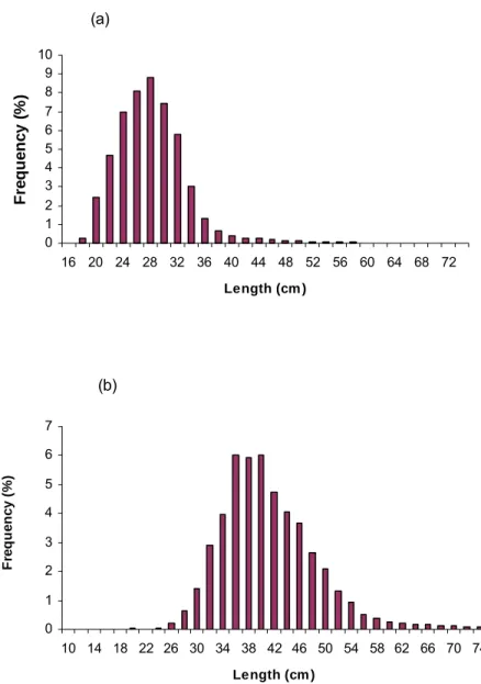
The individual data for length-frequency distribution for each month was unavailable. The monthly survey data, January and February, in Namibia are not examined separately. The length frequency distribution of the biomass survey caught of
M. capensis caught off Namibia during January and February 2003, ranged from 16 cm to
60 cm with a mode of 8.8 % of the population at 28 cm (Figure 2). The length frequency distribution of the commercial fleet of M. capensis caught during January to December in 2003, ranged from 20 cm to 74 cm with a mode of 6 % at 36 cm (Figure 2).
3.1 Otolith Growth Patterns
Up to three false ring termed P3, P2, P1 were visible before the first annual ring (Table 1), but the number of individuals with P3 was very low (n=4). The pattern of false rings continued with decreasing frequency after the first annulus had been formed. The frequency for the ages formed indicated that age 1 had the highest number of individuals (n=145), followed by age 2 (n=141) and age 4 (n=103), respectively (Table 1). The mean calculated otolith diameter (tip to tip) for each translucent ring of hake (Table 1) was similar to mean calculated otolith diameter (tip to tip) separated for fish aged 0 to 4 for
(a) 0 1 2 3 4 5 6 7 8 9 10 16 20 24 28 32 36 40 44 48 52 56 60 64 68 72 Length (cm ) Fr e que nc y ( % ) (b) 0 1 2 3 4 5 6 7 10 14 18 22 26 30 34 38 42 46 50 54 58 62 66 70 74 Length (cm ) F req u en cy ( % )
Figure 2. (a) Length frequency distribution of M. capensis caught during the biomass survey in January and February 2003 off Namibia. Frequencies are presented in percentage of total number in millions km⎯² for January and February. (b) Length frequency distribution of M. capensis caught by the commercial fleet off Namibia in January to December 2003. Frequencies are presented in percentage of total number in million for the year.
The general pattern for the occurrence of rings formed on the otolith of M.
capensis showed more scatter with increasing otolith growth, with f2 (n=27) and f3 (n=8)
as the exception (Figure 3). Averages of otolith diameter (mm) and ages for 5 to 12, showed a greater overlap, similarities between mean and mode (Figure 4). The low frequency of older M. capensis caught during the biomass survey 2003, and the difficulty in interpreting the ring pattern and age estimation, had introduced discrepancies especially in the age 7 to 12 classes (Figure 4). Age 7 and 8 had produced very similar results; where as age 9 and 11 has larger mean, mode, and range compared to age 10 and 12, respectively.
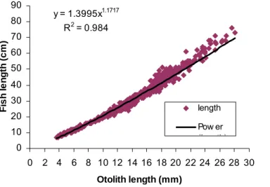
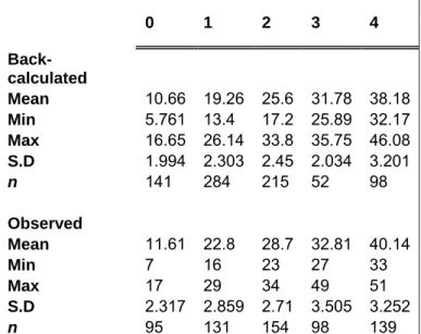
Mean back-calculated lengths at each of the first four annuli (Table 3), indicated the reverse of Lee’s phenomenon, the trend for back-calculated lengths of older fish’s earlier age to be systematically underestimated than the young fish at the same age (Smith, 1983). Mean back-calculated lengths at each of the four annuli were derived from power regression between fish length and otolith diameter, which had a relatively high correlation coefficient, and explained by the following equation (Figure 8):
Table 1: Mean calculated otolith ring diameters (mm) separated for fish aged 0 to 4, for M. capensis collected in Namibian waters. (P3 = 1st pelagic ring, P2 = 2nd pelagic ring, P3 = 3rd pelagic ring; f1; f2; f3;
f4 = False rings; Mean = average calculated for translucent bands (tip to tip) at each age; S.D. = standard deviation; C.V. = coefficient of variation)
Age No. indiv P3 P2 P1 f1 f2 f3 f4 1 2 3 4 0 47 3.9 5.17 5.58 1 145 5.17 6.32 7.43 10.51 10.04 2 141 6.8 7.33 10.38 12.7 9.547 12.46 3 80 7.94 10.11 12.5 14.9 9.26 11.85 14.02 4 103 7.18 11.2 16.4 17.3 9.406 12.2 14.31 16.69 No rings 4 22 117 61 27 8 7 290 220 120 99 Mean 4.53 6.1 7.09 10.55 12.6 15.6 17.3 9.564 12.17 14.17 16.69 S.D 0.9 0.84 0.89 0.463 0.13 1 0.34 0.302 0.21 CV 19.8 13.8 12.6 4.391 1 6.36 3.555 2.486 1.484
Table 2: Mean calculated otolith diameter tip to tip at each translucent band for rings of M. capensis otoliths colleted off Namibian waters during 2003. (P3 = 1st pelagic ring, P2 = 2nd pelagic ring, P3 = 3rd
pelagic ring; f1; f2; f3; f4 = False rings; Mean = average calculated for translucent bands (tip to tip) irrespective of age; S.D. = standard deviation; C.V. = coefficient of variation, q1; q3 = lower and upper quartile, I-range = inter-quartile range)
P3 P2 P1 f1 f2 f3 f4 r1 r2 r3 r4 q1 3.83 5.50 5.80 10.00 12.05 14.35 17.70 8.90 11.50 13.40 16.05 Min 3.60 4.60 4.50 8.20 11.20 14.10 14.40 7.30 10.10 12.10 14.00 Median 4.75 6.35 7.20 10.50 12.50 14.85 17.90 9.50 12.25 14.00 16.70 Max 6.30 7.90 8.90 12.20 13.90 15.70 18.80 12.30 15.20 16.30 19.80 q3 5.78 6.70 7.90 10.90 13.10 15.43 18.25 10.30 12.90 14.80 17.20 Mean 4.85 6.19 6.74 10.44 12.54 14.88 17.57 9.65 12.22 14.11 16.65 I-Range 1.95 1.20 2.10 0.90 1.05 1.08 0.55 1.40 1.40 1.40 1.15 S.D 1.31 0.88 1.24 0.73 0.75 0.66 1.46 0.99 0.94 0.90 0.91 C.V. 26.96 14.29 18.35 7.01 5.98 4.43 8.28 10.24 7.71 6.35 5.45
2 4 6 8 10 12 14 16 18 20 P3 P2 P1 f1 f2 f3 f4 r1 r2 r3 r4 Rings formed O to lit h d iam et er ( m m ) q1 Min Median Max q3 Mean
Figure 3. The proportion of translucent rings found at diameter formed on otoliths of M. capensis during the biomass survey 2003 off Namibian waters.
15 17 19 21 23 25 27 29 Age 5 Age 6 Age 7 Age 8 Age 9 Age 10 Age 11 Age 12 Age (years) O to li th d iam et er ( m m ) q1 Min Median Max q3 Mean
Figure 4. The proportion of ages found at diameter formed on otoliths of M. capensis during the biomass survey 2003 off Namibian waters.
Mean observed lengths-at-age were higher than mean back-calculated lengths for M.
capensis and were probably due to the strong variation in size for each age class (Table
4). The relationship between observed lengths-at-age and predicted lengths-at-age was not significantly different (x² = 0.8748; d.f. = 5; p < 0.05) for the M. capensis population. There was no evidence in location overlap between ages 1 to 4 (annuli), when hyaline
ring formation occurred (Figure 5). This trend was also observed in the annuli of the 1st
and 2nd ages with their respective false rings, f1and f2 (Figure 6).
However, the pelagic rings had shown overlap in their location in M. capensis otoliths, especially during very earlier stages of growth in fish length < 12 cm (Figure 7). The 50 % observed location of hyaline ring formation on the otolith diameter for fish was calculated from the ogives and compared with the mean back-calculated fish length (Table 5).
0 0.2 0.4 0.6 0.8 1 1.2 7 12 17 22 Otolith length C u m u lat ive F ract io n 1st annulus ogive 1st annulus 2nd annulus ogive 2nd annulus 3rd annulus ogive 3rd annulus 4th annulus ogive 4th annulus
Figure 5. Performance: Cumulative distribution of annuli (ages 1 to 4) of M. capensis. These ogives demonstrate the differences in otolith diameter, location frequency between the four ages (annuli) and predicted ring location. An approximate estimate of mid-point or any comparative parameter is described as ‘observed location’ and can easily be made visually from such plots.
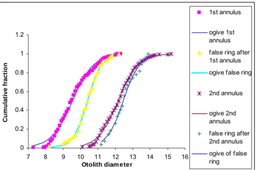
0 0.2 0.4 0.6 0.8 1 1.2 7 8 9 10 11 12 13 14 15 16
Otolith diam eter
C u m u lat ive f ract io n 1st annulus ogive 1st annulus false ring after 1st annulus ogive false ring 2nd annulus ogive 2nd annulus false ring after 2nd annulus ogive of false ring
Figure 6. Performance: Cumulative distribution of 1st and 2nd annuli and their respective false rings of M.
capensis. These ogives demonstrate the differences in otolith diameter, location frequency between the first
two annuli and their respective annuli and predicted ring location. An approximate estimate of mid-point or any comparative parameter is described as ‘observed location’ and can easily be made visually from such plots.
0 0.2 0.4 0.6 0.8 1 1.2 4 5 6 7 8 9 10 11 12 13
Otolith diam eter
C u m u lat ive F ract io n P2 ring ogive P2 ring P1 ring ogive P1 ring 1st annulus ogive 1st annulus
Figure 7. Performance: Cumulative distribution of pelagic rings and 1st annulus of M. capensis. These
ogives demonstrate the differences in otolith diameter, location frequency between the pelagic rings and 1st
annulus and predicted ring locations. An approximate estimate of mid-point or any comparative parameter is described as ‘observed location’ and can easily be made visually from such plot
y = 1.3995x1.1717 R2 = 0.984 0 10 20 30 40 50 60 70 80 90 0 2 4 6 8 10 12 14 16 18 20 22 24 26 28 30 Otolith length (mm) F is h l e n g th (c m ) length Pow er (l th)
Figure 8. Power regression between fish length and otolith diameter (length) for M. capensis during biomass survey in 2003 in Namibia.
Table 3: The mean back-calculated fish lengths at ages for M. capensis. Age P3 P2 P1 r1 f1 r2 f2 r3 f3 r4 f4 0 6.34 9.152 10.76 1 9.07 11.59 14.04 20.22 20.95 2 11.94 13.67 19.05 19.88 25.99 26.08 3 14.87 18.55 20.46 24.8 25.52 32.33 32.33 4 13.55 19.2 22.18 26.04 31.22 38.18 39.15 mean 7.7 10.89 13.38 19.26 20.87 25.61 25.8 31.78 32.33 38.18 39.15 Table 4: Mean, minimum and maximum lengths-at-age (cm) and statistics for observed actual and back-calculated ages 0 to 4 years for M. capensis in 2003.
0 1 2 3 4 Back-calculated Mean 10.66 19.26 25.6 31.78 38.18 Min 5.761 13.4 17.2 25.89 32.17 Max 16.65 26.14 33.8 35.75 46.08 S.D 1.994 2.303 2.45 2.034 3.201 n 141 284 215 52 98 Observed Mean 11.61 22.8 28.7 32.81 40.14 Min 7 16 23 27 33 Max 17 29 34 49 51 S.D 2.317 2.859 2.71 3.505 3.252 n 95 131 154 98 139
Table 5: Observed mean otolith diameter, mean back-calculated fish length, mean otolith diameter and fishlength calculated from ogives. (Mean OD = Mean observed diameter in mm; Mean B.F = Mean back-calculated fish length in cm; Mean OD from ogives = Mean otolith diameter back-calculated from Ogives; Mean F from Ogives = Mean fish length calculated from ogives).
P3 P2 P1 f1 f2 f3 f4 r1 r2 r3 r4 Mean OD 4.9 6.2 6.7 10.4 12.5 14.9 17.6 9.7 12.2 14.1 16.7 Mean B.F 7.7 11 13 20.9 25.8 32.3 39.2 19 25.6 31.8 38.2 Mean OD from Ogives 3.9 6.3 7.2 10.5 12.5 14.4 17.9 9.5 12.2 14 16.7 Mean F from Ogives 6.9 12 14 22 27 31.9 41.1 20 26.2 30.8 37.9
3.2 Age Determination
Age estimates were produced from 757 otoliths after the rejection of unreadable or damaged otoliths (n=47). Thus 94 % of the whole sample was successfully analysed. The percent agreement calculated between two readings was 66.3 % in otoliths of Cape hake with ages ranging from 0 to 13 years. The repeated age estimates were relatively precise with 70 % of the otoliths assigned the same age for young individuals, in each round; 100 % of the estimates ± 0 year; 76 % ± 1 year; 73 % ± 2 years; 73 % ± 3 years. Typically precision decreased with increasing age. The greatest discrepancy encountered was age 7 which had a 0 % percentage agreement. No individuals were assigned the age 11 for each round of age estimations.
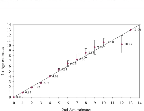
The measurement of average CV between the readings was 12 %. In Table 6, the measurements of CV between readings for ages 0 to 13 are shown. Visual examination of all age estimations was very precise for M. capensis estimated at 0 to 13 years of age; the 95 % confidence intervals associated with age class estimates overlapping the 1:1 ratio line (Figure 9). However, the age class 11 was slightly underestimated in comparison with the other age classes. Bowker’s test result for individuals older than 2 years, (x² = 21.78; d.f. = 30; p = 0.86) was used to compare the two readings and had indicated that Cape hake individuals was assigned ages without systematic disagreement (bias); thus the hypothesis of symmetry is accepted and the disagreement between the readings was due to simple random error.
Table 6: CV for each age group of M. Capensis for 2003. CV is noted as a fraction of the age group. Year 1 2 3 4 5 6 7 8 9 10 12 13 Overall 2003 0.28 0.12 0.08 0.1 0.1 0.11 0.16 0.12 0.1 0.04 0.12 0 0.1208 0.00 0.87 1.92 2.74 4.02 5.31 6.52 7.30 8.53 9.67 10.60 10.25 13.00 0 1 2 3 4 5 6 7 8 9 10 11 12 13 14 0 1 2 3 4 5 6 7 8 9 10 11 12 13 14 2nd Age estimates 1s t A ge es ti m at es
Figure 9. Age-Bias plot of otoliths (n=757) for M. capensis with the 1:1 ratio shown. Mean 1st Age
estimates was plotted with a 95 % confidence interval.
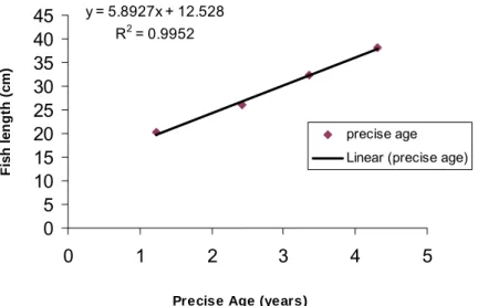
The marginal increment analysis for data had indicated decreasing absolute marginal distance, AMD (the distance between edge and last annulus) with increasing age (Table 7). The relative marginal distance (RMD) for first four annuli (Table 8), had indicated the precise ages for Cape hake and was used to predict fish length from back-calculated data. The linear regression of fish length-at-precise age had produced a very high correlation coefficient, R² = 0.9952 and yielded the following formula (Figure 10):
However, the observed fish length-at-precise age signifies an even higher correlation coefficient, R² = 0.991 with the formula (Figure 11):
L = 6.7046 × precise age + 12.656
The assumption that most of the hyaline bands had formed up to age 4, implied that the mean relative marginal distance (RMD) values was formed a year ago prior to capture of Cape hake. Therefore, the month in which the hyaline ring had formed, since the capture date was from January to end of February, was:
r1 = 0.2 × 1 year = 0. 2 × 12 months = 2.4 months; less than two and half months prior to capture between October and November 2002;
r2 = 0.4 × 1 year = 0.4 × 12 months = 4.8 months; approximately 5 months prior to capture between August and September;
r3 = 0.3 × 1 year = 0.3 × 12 months = 3.6 months; three and half months prior to capture between September and October;
r4 = o.3 × 1 year = 0.3 × 12 months = 3.6 months; three and half months prior to capture between September and October.
3.3 Age Structure
The 2003 Age Length Key (ALK) calculated from data of biomass survey is given in Table 9, and applied to the biomass survey length-frequency distribution to calculate the age distribution, the catch-at-age for 2003, shown in Figure 12. The 2003 Age length key (ALK) calculated from data of biomass survey was applied to the commercial length-frequency distribution to calculate the age distribution, the catch-at-age for 2003, shown in Figure 13.
Table 7: Mean absolute marginal distance for annuli calculated during Cape hake survey in 2003. Age r1 r2 r3 r4 1 1.42 2 1.01 3 0.65 4 0.91
Table 8: Relative marginal distance, RMD for annuli calculated during Cape hake survey in 2003.
Age r1 r2 r3 r4 1 0.23 2 0.41
3 0.356
y = 5.8927x + 12.528 R2 = 0.9952 0 5 10 15 20 25 30 35 40 45 0 1 2 3 4 5
Precise Age (years)
F is h l e ng th (c m ) precise age Linear (precise age)
Figure 10. The linear regression plot of back-calculated total fish length against precise age. The marginal increment analysis estimation was used to acquire the precise age estimations and for the 2003 hake survey.
y = 6.7046x + 12.656 R2 = 0.9991 0 5 10 15 20 25 30 35 40 45 0 1 2 3 4 5
Precise Age (years)
Fi s h Le n g th ( c m) precise age Linear (precise age)
Figure 11. The linear regression plot of observed total fish length against precise age. The marginal increment analysis estimation was used to acquire the precise age estimations for the 2003 hake survey.
Table 9: 2003 Age length key (ALK) for M. capensis AGE GROUP (year)
Length class (cm) 0 1 2 3 4 5 6 7 8 9 1 0 1 1 1 2 1 3 Grand Total <8 2 2 8 5 5 10 26 26 12 31 31 14 19 19 16 9 1 10 18 2 11 13 20 13 13 22 33 33 24 38 8 46 26 24 26 50 28 8 44 11 63 30 3 39 13 55 32 20 23 43 34 17 21 2 40 36 21 16 37 38 7 34 41 40 1 27 28 42 2 24 1 27 44 25 5 30 46 8 16 1 25 48 1 21 2 24 50 1 1 21 4 27 52 1 15 2 18 54 10 4 14 56 5 9 1 1 16 58 2 5 2 9 60 1 2 3 4 10 62 3 2 4 9 64 1 3 1 5 66 1 3 1 5 68 1 2 2 1 6 70 1 1 2 72 2 1 1 1 1 6 74 1 1 76 1 1 1 3 78 1 1 2 80 1 1 Grand Total 94 13 1 154 100 139 97 32 10 17 6 6 2 5 2 795 Mean Length 13 23 29 39 43 50 54 6 1 6 2 6 9 6 9 7 4 7 4 7 4
0 20000 40000 60000 80000 100000 0 1 2 3 4 5 6 7 8 9 10 11 12 13 Age (year) N u m b er cau g h t ( m il li o n s)
Figure 12. The catch-at-age for 2003 calculated from the biomass survey length frequency distribution and the ALK. 0 200 400 600 800 1000 1200 0 1 2 3 4 5 6 7 8 9 10 11 12 13 Age (year) N u m b er cau g h t ( m il li o n s)
Figure 13. The catch-at-age for 2003 calculated from the commercial fleet length frequency distribution and the ALK.
3.4 Growth Rate Determination
The von Bertalanffy growth parameters were estimated for M. capensis by non-linear regression analysis fitting the von Bertalanffy growth function and the following parameters and Residual sum of squares (RSS) was determined:
∞
L = 123.13; K = 0.07; = -1.5; RSS = 9963 t0
The resultant growth function was:
=123.13
[
1− −0.07(t+1.5)]
t e
L
The growth curve for M. capensis are presented in Figure 14. The weight-length relationship was presented by the following parameters:
a = 0.0076; b = 2.9739
The resultant non-linear power regression weight-length relationship function resulted with a very high correlation coefficient, R² = 0.99, illustrated in Figure 15, was:
0.0076 2.9739
L Wt =
The resultant non-linear power regression weight-at-age relationship functions based on the von Bertalanffy growth function parameters and M. capensis biological information from the biomass survey, indicated in Figure 16.
Figure 17, has shown that the age at 50 % maturation, for M. capensis was 1.67 years
during 2003 assessment.
5 . 0
0 5 10 15 20 25 30 35 40 45 50 55 60 65 70 75 80 0 1 2 3 4 5 6 7 8 9 10 11 12 13 14 15 Age (years) Le n g th (c m ) length VBGF
Figure 14. Estimates of mean length-at-age for M. capensis, based on the von Bertalanffy growth function parameters. y = 0.0076x2.9739 R2 = 0.9908 0 500 1000 1500 2000 2500 3000 3500 4000 0 5 10 15 20 25 30 35 40 45 50 55 60 65 70 75 80 Length (cm ) We ig h t ( g ) w eight Pow er (w eight)
Figure 15. The non-linear power regression relationship between fish weight and fish length for M.
0 500 1000 1500 2000 2500 3000 3500 0 1 2 3 4 5 6 7 8 9 10 11 12 13 14 15 16 Age (year) Fi s h w e igh t ( g ) w eight mean w eight-at-age
Figure 16. Fish weight against age for M. capensis obtained from the 2003 biomass survey fitted with a power curve. 0 0.2 0.4 0.6 0.8 1 1.2 0 1 2 3 4 5 6 7 8 9 10 11 12 13 14 Age (years) % M a tur ity (P ) M.capensis M.capensis ogive
3.5 Relationships between otolith weight, age and fish length
The regression analysis of the relationship between otolith weight (OW) and age indicated linearity;
OW = 0.0384 × age + 0.0074
And provided the best fit, with a correlation coefficient, R² = 0.939 (Figure 18). A regression analysis of fish length-at-age yielded;
L = -0.2372 × (age)² + 8.1386 × age + 12.887
Explaining 94 % of variability in length, shown in Figure 19. The linear regression analysis of otolith diameter-at-age yielded;
L = -0.1348 × (age)² + 3.2312 × age + 6.9531
And with a correlation coefficient, R² = 0.9332, Figure 20. The relationship between otolith weight and age (Figure 16) had a similar correlation coefficient than that otolith length and age. The fish length-age relationship yielded a similar correlation coefficient than that between fish length and age. Therefore, for M. capensis it is precise to use otolith weight to estimate age.
The relationship between otolith weight and fish length shown, in Figure 21, indicated a non-linear polynomial function:
=5∃−05 2 +0.0025 −0.027
x x
OW
And a relatively high correlation coefficient, R² = 0.9768. The relationship between otolith weight and otolith length shown in Figure 22, yielded a non-linear power function:
OW =0.0001
( )
OL 2.5498With a high correlation coefficient, R² = 0.9935. Therefore, both fish length and otolith length can be used to efficiently predict otolith weight.
y = 0.0384x + 0.0074 R2 = 0.9392 0 0.05 0.1 0.15 0.2 0.25 0.3 0.35 0.4 0.45 0.5 0.55 0 1 2 3 4 5 6 7 8 9 10 11 12 13 14 Age (years) Ot o li th we ig h t (g ) w eight Linear (w eight)
Figure 18. Linear regression relationship for otolith weight against age of M. capensis in 2003.
y = -0.2372x2 + 8.1386x + 12.887 R2 = 0.9419 0 5 10 15 20 25 30 35 40 45 50 55 60 65 70 75 80 85 0 1 2 3 4 5 6 7 8 9 10 11 12 13 14 Age (years) Fi s h l e n g th (c m ) length Poly. (length)
y = -0.1348x2 + 3.2312x + 6.9531 R2 = 0.9332 0 2 4 6 8 10 12 14 16 18 20 22 24 26 28 30 0 1 2 3 4 5 6 7 8 9 10 11 12 13 14 Age (years) O to li th d iam et er ( m m ) OtoLength Poly. (OtoLength)
Figure 20. Linear regression relationship of otolith diameter-at-age for M. capensis in 2003.
y = 5E-05x2 + 0.0025x - 0.027 R2 = 0.9768 0 0.05 0.1 0.15 0.2 0.25 0.3 0.35 0.4 0.45 0.5 0.55 0 5 10 15 20 25 30 35 40 45 50 55 60 65 70 75 80 85 Fish length (cm ) Ot o li th we ig h t (g ) w eight Poly. (w eight)
y = 0.0001x2.5498 R2 = 0.9935 0 0.05 0.1 0.15 0.2 0.25 0.3 0.35 0.4 0.45 0.5 0.55 0.6 0 2 4 6 8 10 12 14 16 18 20 22 24 26 28 30 Otolith w eight (g) O tol it h l e ng th ( mm) w eight Pow er (w eight)
4. Discussion
The modal size in the biomass survey for 2003 (mode = 28 cm) differed significantly with the commercial fleet’s modal size (mode = 36 cm). The biomass survey’s range had not included a significant part of the older age classes. Whilst the commercial fleet targets larger fish, the data shows that they are catching smaller fish. The larger individuals (<50 cm) were less represented in the recent years of sampling. The differences in survey and commercial size of M. capensis had suggested that it was impractical to determine a true modal size and hence precise estimates of fishing mortality can not be made with survey results.
4.1 Otolith Growth Patterns
M. capensis otoliths showed that the first annual translucent ring is preceded by
three pelagic rings. The first pelagic ring laid down at 8 cm fish mean length was rarely visible. The second pelagic ring had a higher occurrence at 11 cm fish mean length.
Whilst the 3rd pelagic ring, which was laid down just before the first annual translucent
ring, had an even higher occurrence at 13 cm mean fish length. These findings agree well with studies of Gordoa et al. (2001), which observed M. capensis forming translucent rings throughout their first year of growth and depending on the month, the translucent ring would be of shorter or longer duration. They had observed 140 day old fish between 6-11cm; 160 day old fish between 14-18 cm; and 1 year old fish between 18 and 22 cm. The formation of translucent rings in the South Atlantic had been associated with hatching during spring (Botha, 1971; Piñeiro and Hunt, 1989).
The observed first annual hyaline ring was laid down at 22 cm mean fish length. The observed size range of fish when the first annual translucent ring had been laid down was very broad (16-29 cm) that is probably due to error in otolith interpretation. The mean back-calculated length at ages corresponding to translucent ring formation had shown similar results compared to the actual observed length at ages (x² = 0.8748; d.f. = 5; p<0.05). However, the overall mean observed length at age was slightly higher than the mean back-calculated length at age, likely due to the strong variation in size for each year class.
The back-calculated size range of fish when the first annual translucent ring was laid down was 13-26 cm with a mean of 19 cm. In this study, several false rings had been observed after the first four annuli, at a mean back-calculated fish length of 21 cm, 26 cm; 32 cm, 39 cm, respectively. This had represented a break in biological and or environmental significance after the first, second, third and fourth annuli had been laid down. M. capensis daily migratory pattern, variations in water temperature, feeding pattern (Morales-Nin, 1987, Pannella, 1980) might offer an explanation for the occurrence of these false rings.
The mean back-calculated length at age 1 (19 cm) confirms studies of Gordoa et
al. (2001), who had estimated a mean length of 20 cm. Morales-Nin 1(986), had
estimated a mean length of 22 cm at age 1 for M. capensis. Slight differences in back-calculated and actual observed length at age 1 can be attributed to different otolith interpretation. Growth of M. capensis seems to be greater than growth of the European hake. Gordoa et al. (2001), had shown that length at age 1 for Cape hake was higher than that of European hake and this study confirms this trend.
The average calculated otolith diameter (tip to tip) for all translucent bands from the sample of M. capensis otoliths (Table 2), provided similar results as that of the average calculated otolith diameter (tip to tip) for translucent bands separated by age 0 to 4 (Table 1). Therefore, otolith diameter (tip to tip) for all translucent bands need not be separated by age group. This implies that overall measurements of translucent bands can be used to indicate where to count annuli. Although effects of natural mortality and fishing mortality have to be evaluated for M. capensis, the absence of Lee’s phenomenon from back-calculated data implies that size-selective mortality was not present in this population (Boehlert et al., 1989). Since the commercial fleet targets larger individuals, indicative of the low numbers of larger individuals (Figure 2), and with the absence of Lee’s phenomenon the data is more suggestive towards evidence of cannibalism within the Cape hake population. This confirms well with previous studies emphasizing the importance of cannibalism in this species (Macpherson, 1980; Prenski, 1980; Roel and Macpherson, 1988; Roux 2006).
The cumulative distribution is a sigmoid curve. The performance of this method was illustrated by translucent ring location of different zones and compares the predicted location. The cumulative distribution of translucent ring formation illustrated the location and formation differences in the M. capensis otolith. Any given ‘observed location’ parameters can be estimated easily from the cumulative distribution. The cumulative distribution, an ogive, for all ages (1 to 4) calculated from the frequency distribution had shown that increment growth in the first year was the highest (Figure 5). Thereafter, the increment growth slows down and the increment width was smaller (Figure 5). These
ogives (Figure 5 to Figure 7) had illustrated the differences in location between the first
and second annulus and its subsequent false rings. The 1st and 2nd annuli and their
respective false rings had the highest number of individual M. capensis otoliths (Table 1).
This signifies the existence of the false rings after the 1st and 2nd annulus, respectively.
The existence of false rings effectively increases the difficulty of age estimations. However, this result had shown that otolith diameter can effectively predict the annulus and false ring growth of the M. capensis otolith. Given that no overlap in ogives for these rings was visible, thus the first and second annuli and its subsequent false rings have not been identified interchangeable. Slight overlap, however had been observed in the two pelagic rings especially at smaller otolith size. This had illustrated that the pelagic rings, especially smaller than 6 mm otolith diameter length has a greater probability of interchangeable otolith term interpretation. Mean observed, back-calculated and cumulative distributions (Table 4 and Table 5) length at age 1 values was relatively similar compared to seal scat analysis studies done by Roux (2004). According to this author, the 2002 cohort had first appeared in the diet of the Cape fur seal at 8 cm fish length. By the end of December 2003, after completion of its first year of growth, the Cape hake had reached a mean length of 21 cm. Therefore, in careful consideration of results, this current study has successfully determined distinct growth rings on the whole sagittal otolith.
4.2 Age Determination
Precision describes the degree to which data generated from repetitive measurements of age differ from one another (Campana, 2001). Statistically this concept is referred to as dispersion. Accuracy refers to the correctness of the data; unless the true age is known and method validated, accuracy cannot be evaluated (Campana, 2001). High precision does not imply high accuracy and vice versa (Campana, 2001). Ageing errors can be either random or biased, reflecting some combination of process and interpretation error. Although bias can be avoided through validation studies and quality control, random error is virtually inevitable (Campana, 2001). Age estimates of M.
capensis based upon actual observed annuli were relatively precise, with the precision
values comparing favourably to studies of M. capensis. Generally, the CV values was higher in younger age classes and lower in older age classes (Table 10), in which CV values was compared and findings agreed well with studies done by Wilhelm (2006), whereby the author had pooled survey data over a five year period from 2000 to 2005. These findings, however are in contrast to comments by Campana et al., (1995), who had illustrated that at older ages, CV and APE values are expected to rise due to increased difficulty in interpretation of narrow annuli associated with decreased growth rates as the fish approaches asymptotic size. In this study, difficulty in reading and interpreting the older M. capensis ages was a certainty; therefore increment width had been measured for the first four ages only, beyond age 4 increment widths was extremely doubtful. The high CV values for age 1 can be ascribed to the difficulty in interpretation of M. capensis otoliths; thus necessitates the establishment of more precise ageing estimation methods to
clearly distinguish between pelagic rings and the first and second annuli within the M.
capensis population.
Several studies had pointed out the importance of ageing precision without systematic disagreement among readers or readings (Campana and Jones, 1992). Hoening
et al., (1995) had described the test of symmetry developed by Bowker (1948), which
determines if systematic difference exists between paired ages assignment and considers only the samples where the age was not agreed upon. Comparisons are made on the diagonal, i.e. fish with ages (1, 2) are compared with fish having ages (2, 1). Bowker’s test was used to determine the type of error, systematic (bias) or random error was indicated within results. The lack of an age bias in CV values, Bowker’s test (x² = 21.78; d.f. = 30; p = 0.86), had indicated that otoliths can provide precise ages for individuals older than 2 years.
Marginal increment analysis had indicated that annuli were laid down during spring (August to November) which agrees favourably with previous studies (Botha, 1971; Piñeiro and Hunt, 1989) which had indicated that there is a seasonal pattern for the opaque and translucent ring formation corresponding to fast growth in autumn and slow growth in spring. Although the hyaline zone can be formed throughout the year, studies have shown that in respect to seasonal zone formation, hyaline formation occurs in periods of maximum reproductive activity (Grinols and Tillman, 1970; Botha, 1971). Spawning in Namibia for Cape hake has been estimated to be around August to November (Gordoa et al. 2001). Therefore, this result for the approximate time of annulus formation, during peaks of spawning agrees with the above findings.
Ideally, annulus formation should be verified with monthly samples across a longer time series and across many age classes (Campana, 2001). The lack of monthly sampling in Namibia prior to this study had however restricted conventional marginal analysis technique and had made it impractical to compare monthly differences across ages. The results can however be of great important application in future marginal increment analysis.
The linear regression analysis of observed and back-calculated length at precise age estimates had illustrated a very high correlation coefficient, which had highlighted the importance for monthly samples across a broad range of ages for marginal increment analysis.
4.3 Age Structure
The use of stock assessment models in providing advice for the management of fish stocks requires information on the age structure of stocks (Campana and Thorrold, 2001). Generally, two methods are used to obtain estimates of catch-at-age (Mesnil, 2002). When fish is sampled randomly and age estimations made of all fish sampled. The proportions at age in the sample are taken as the estimates of those in the population being sampled (simple random sampling). An alternative method utilized, is when a large sample of fish is randomly sampled and the fish’s length recorded, a sub-sample of the large sample is randomly selected (typically stratified by size classes, i.e. a fixed number is taken at each age) and its age estimated (Mesnil, 2002).
From visual evaluation of the catch-at-age data from the survey, it’s clear that the survey had caught millions more smaller fish than the commercial fleet (Figure 12 and Figure 13). The restriction of older age classes in the survey and the commercial fleet