i
UNIVERSIDADE
DA
BEIRA
INTERIOR
Engenharia
4D Fuel Optimal Trajectory Generation from
Waypoint Networks
Kawser Ahmed
Dissertação para obtenção do grau de mestre em
Engenharia Aeronáutica
(
Ciclo de estudos integrado)
Orientador: Prof. Doutor Kouamana Bousson
iii I would like to express my sincere appreciation to Professor Kouamana Bousson for his support and guidance throughout this thesis and throughout my education at The University of Beira Interior. Finally, I would like to thank my family and friends for their support during my education at The University of Beira Interior.
v The purpose of this thesis is to develop a trajectory optimization algorithm that finds a fuel optimal trajectory from 4D waypoint networks, where the arrival time is specified for each waypoint in the network. Generating optimal aircraft trajectory that minimizes fuel burn and associated environmental emissions helps the aviation industry cope with increasing fuel costs and reduce aviation induced climate change, as CO2 is directly related to the amount of fuel burned, therefore
reduction in fuel burn implies a reduction in CO2 emissions as well.
A single source shortest path algorithm is presented to generate the optimal aircraft trajectory that minimizes the total fuel burn between the initial and final waypoint in pre-defined 4D waypoint networks. In this work the 4D waypoint networks only consist of waypoints for climb, cruise and descent phases of the flight without the takeoff and landing approach. The fuel optimal trajectory is generated for three different lengths of flights (short, medium and long haul flight) for two different commercial aircraft considering no wind.
The Results about the presented applications show that by flying a fuel optimal trajectory, which was found by implying a single source shortest path algorithm (Dijkstra’s algorithm) can lead to reduction of average fuel burn of international flights by 2.8% of the total trip fuel. By using the same algorithm in 4D waypoints networks it is also possible to generate an optimal trajectory that minimizes the flight time. By flying this trajectory average of 2.6% of total travel time can be saved, depends on the trip length and aircraft types.
Keywords
Fuel Conservation; Cost Index; Dijkstra’s algorithm; 4D Waypoint navigation; Base of Aircraft Data (BADA);
vii Esta tese tem como objetivo desenvolver um algoritmo de otimização de trajetória que permita encontrar uma trajetória de combustível ótima em uma redes de waypoint em 4D, onde o tempo de chegada é específico para cada waypoint da rede. Ao criar uma trajetória ótima que minimize o consumo de combustível da aeronare e as suas respetivas emissões poluentes, ajuda a indústria da aviação não só a lidar com o aumento nos custos dos combustíveis, bem como a reduzir a sua contribuição nas alterações climáticas, pois o CO2 está diretamente relacionado com a quantidade
de combustível queimado, logo uma redução no seu consumo implica que haja também uma redução nas emissões de CO2.
O algoritmo “single source shortest path” é utilizado de forma a gerar uma trajetória ótima, que minimize o consumo de combustível entre o waypoint inicial e final de redes pré-definida de waypoint em 4D. Neste trabalho, esta redes consiste num conjunto de waypoints inseridos apenas nas fases de voo de subida, cruzeiro e descida, ignorando assim as fases de descolagem e aterragem. A trajetória de combustível ótima é criada para dois aviões comerciais diferentes em três distâncias de voo também diferentes (voo curto, médio e longo), sem considerar o vento.
Os resultados deste trabalho mostram que ao voar numa trajetória de combustível ótima, obtida através do algoritmo “single source shortest path” (Dijkstra’s algorithm), é possível reduzir o consumo total de combustível numa média de 2.8%, em voos internacionais. Utilizando o mesmo algoritmo numa rede de waypoints em 4D é também possível encontrar uma trajetória ótima que minimize o tempo de voo numa media de 2.6% do tempo total, consoante a distância da viagem e do tipo de aeronave.
Palavras-chave
Conservação de combustível; Cost Index; Dijkstra’s algorithm; Navegação por waypoints em 4D; Base of Aircraft Data (BADA);
ix List of Figures………..xi List of Tables………xiii List of Acronyms ………..xv List of Symbols………xvii 1 Introduction ... 1 1.1 Motivation ... 1
1.2 Fuel Saving in Different Phases of Commercial Flight ... 3
1.2.1 Cruise Phase ... 4
1.2.2 Takeoff and Climb Phase ... 6
1.2.3 Descent and Approach Phase ... 7
1.3 Trajectory Optimization ... 9
1.4 Objectives ... 10
1.5 Outline ... 11
2 Dijkstra’s Algorithm ... 13
2.1 Pseudo-code of Dijkstra’s Algorithm ... 14
2.2 Representation of Graph ... 15
2.3 Implementation of Dijkstra’s in Flight Trajectory Optimization ... 16
3 Modeling of the 4D Waypoints Network ... 17
3.1 Navigation Model ... 18
3.2 Flight Constraints ... 18
3.3 Arrival Time of Each Waypoint ... 19
3.4 Engine Thrust ... 21
3.4.1 Maximum Climb and Take-off Thrust ... 21
3.4.2 Maximum Cruise Thrust ... 22
3.4.3 Descent Thrust ... 22
3.5 Fuel Consumption Model ... 23
3.5.1 Thrust Specific Fuel Consumption ... 23
3.5.2 Nominal Fuel Flow Rate ... 24
3.6 Consumed Fuel Between Waypoints ... 25
4 Optimal Trajectory Generation ... 27
4.1 Selection of Flights for Analysis ... 27
4.2 Selection of Aircraft for Analysis ... 28
4.3 Fuel Optimal Trajectory Generation ... 29
4.4 Time Optimal Trajectory Generation ... 29
x
5 Simulation and Result ... 33
5.1 Short Haul Flight ... 33
5.1.1 Fuel Optimal Trajectory ... 35
5.1.2 Time Optimal Trajectory ... 36
5.2 Medium Haul Flight ... 37
5.2.1 Fuel Optimal Trajectory ... 38
5.2.2 Time Optimal Trajectory ... 39
5.3 Long Haul Flight ... 40
5.3.1 Fuel Optimal Trajectory ... 42
5.3.2 Time Optimal Trajectory ... 43
6 Conclusion and Discussions ... 45
6.1 Future work ... 46
xi
Figure 1-1: Fuel Prices over the years in Dollar ... 1
Figure 1-2: Effect of the winglet on the vortex ... 2
Figure 1-3: Different phases of commercial flights from takeoff to landing. ... 4
Figure 1-4: Comparison of different cruise speeds ... 4
Figure 1-5: Optimum altitude determination at constant Mach number ... 5
Figure 1-6: Descent profile at given IAS ... 7
Figure 1-7: Typical descent phase of commercial flight ... 8
Figure 2-1: Pseudo-code for Dijkstra’s algorithm ... 14
Figure 2-2: The execution of Dijkstra's algorithm ... 15
Figure 2-3: Representation of graph G into matrix ... 16
Figure 5-1: 3D fuel optimal trajectory in geocentric coordinates for short haul flight. ... 35
Figure 5-2: 3D time optimal trajectory in geocentric coordinates for short haul flight. ... 36
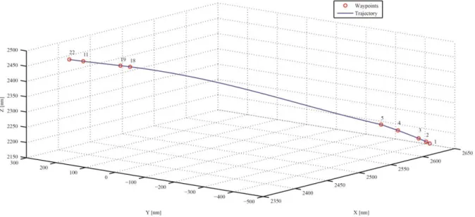
Figure 5-3: 3D fuel optimal trajectory in geocentric coordinates for medium haul flight. ... 39
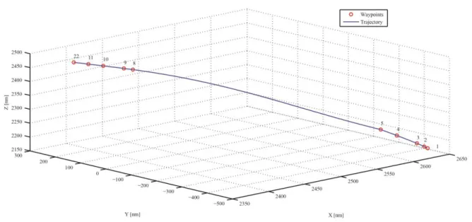
Figure 5-4: 3D time optimal trajectory in geocentric coordinates for medium haul flight. ... 40
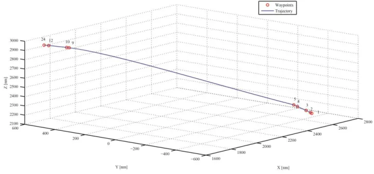
Figure 5-5: 3D fuel optimal trajectory in geocentric coordinates for long haul flight. ... 42
xiii
Table 1-1: ECON cruise Mach in different cruise wind conditions ... 5
Table 1-2: Impact of takeoff flap settings on fuel burn ... 6
Table 1-3: Fuel saving potential of two climb profile ... 7
Table 1-4: Fuel savings estimates for delayed flaps approach procedure ... 9
Table 4-1: Characteristics of airplane A1 and airplane A2 ... 28
Table 5-1: List of waypoints in 1st trajectory of short haul flight ... 34
Table 5-2: List of waypoints in 2nd trajectory of short haul flight ... 34
Table 5-3: Total fuel consumed in different trajectories for short haul flight. ... 35
Table 5-4: Total time needed in different trajectories for short haul flight. ... 36
Table 5-5: List of waypoints in 1st trajectory of medium haul flight ... 37
Table 5-6:List of waypoints in 2nd trajectory of medium haul flight ... 38
Table 5-7: Total Fuel consumed in different trajectories for medium haul flight. ... 38
Table 5-8: Total time needed in different trajectories for medium haul flight. ... 39
Table 5-9: List of waypoints in 1st trajectory of long haul flight ... 41
Table 5-10: List of waypoints in 2nd trajectory of long haul flight ... 41
Table 5-11: Total Fuel consumed in different trajectories for long haul flight. ... 42
xv AGL Above Ground Level
ATC Air Traffic control BADA Base of Aircraft Data
CAEP Committee on Aviation Environment Protection CAS Calibrated Air Speed
CDU Control Display Unit
CI Cost Index
FMC Flight Management Computer GHG Green House Gas
GPS Global Positioning System GTF Geared Turbofan Technique IAS Indicated Air Speed
ICAO International Civil Aviation Organization IPCC Intergovernmental Panel on Climate Change LRC Long Range Cruise
MRC Maximum Range Cruise
SID Standard Instrument Departure
SR Specific Range
STAR Standard Terminal Arrival Route TAS True Air Speed
TOD Top of Descent
xvii
Arrival time tolerance interval
Latitude [deg]
Flight path angle [deg]
Thrust specific fuel consumption [kg/(min.KN)]
Longitude [deg]
Air density [kg/m3]
Arrival time at waypoint [min]
Heading [deg]d
Distance between waypoints [nm]T
Temperature deviation from standard atmosphere [K]a
Acceleration [m/s]a
Earth semi major axis [nm]L
C
Lift coefficient 1 fC
, 2 fC
Thrust specific fuel consumption coefficient3
f
C
,4
f
C
Descent fuel flow coefficientcr
f
C
Cruise fuel flow correction coefficient,1 c T
C
, ,2 c TC
, ,3 c TC
Climb thrust coefficient,4 c T
C
, ,5 c TC
Thrust temperature coefficientr
c
T
C
Maximum cruise thrust coefficient.
des app
T
C
Approach thrust coefficient. high
des
T
C
High altitude descent thrust coefficient. ld
des
T
C
Landing thrust coefficient.low
des
T
C
Low altitude descent thrust coefficientD
Dragdf
Consumed fuel between waypoints [kg]d
Travel time between waypoints [min]E
Edges between verticese
Eccentricity/
ap ld
f
Approach and landing fuel flow rate [kg/min]cr
f
Cruise fuel flow rate [kg/min]min
f
Minimum fuel flow rate [kg/min]nom
f
Nominal fuel flow rate [kg/min]G
Graphxviii
,
p des
H
Transition altitude [feet]d
M
Descent Mach number [Mach]P
Waypoint eR
Earth radius [nm]S
Wing area [m2]s
Source vertexThr
Thrust [KN](
Thr
cruise)
MAX
Maximum cruise thrust [KN],app
des
Thr
Approach thrust [KN],
des high
Thr
High altitude descent thrust [KN],ld
des
Thr
Landing thrust [KN],low
des
Thr
Low altitude descent thrust [KN]maxclimb
Thr
Maximum climb thrust [KN]maxclimb
(
Thr
)
ISA
Maximum climb thrust at standard atmospheric condition [KN]V
Flight velocity [Knots]V
Vertices of the graphCAS
V
Calibrated air speed [Knots]TAS
V
True air speed [Knots]W
Aircraft Nominal weight [kg]w
Weight of the graph, ,
1
Chapter 1
1 Introduction
1.1 Motivation
Fuel saving on flight mission for commercial aircraft becomes an important factor nowadays in aviation mainly because of two reason, one is ever increasing fuel prices and other is to reduce the emission rates of greenhouse gases (GHG) into the atmosphere.
Improving aircraft operational efficiency has become a dominant theme in air transportation, as the airlines around the world have seen the price of fuel has risen sharply during the last decades (figure 1-1). The fuel cost represents around 30% of the operating costs for the airlines, thus the airlines are looking for different ways to reduce the flight operating costs by reducing the fuel consumption during the flight, also mounting scientific evidence of global climate change has spurred increased awareness of the importance of manmade greenhouse gas (GHG) emissions such as CO2, resulting in significant pressure to reduce emissions. International civil aviation
organization (ICAO) and committee on aviation Environmental protection (CAEP’s) estimated that currently, aviation accounts for about 2% of total global CO2 emissions and about 12% of the CO2 from
all transportation source [1], and by 2050, aviation’s contribution could increase to 5% of the total human generated global warming. In terms of climate change, the Intergovernmental Panel on climate change (IPCC) estimated an increase in the earth’s temperature of approximately 1.6 degrees Fahrenheit by 2050, of which about 0.09 degrees would be attributed to aviation. This increased fuel
2
prices and environmental concerns have pushed airlines to reduce fuel consumption and to find margins for performance improvements [2].
Technological improvement such as development of more efficient engines, lighter materials, new aerodynamic designs, and the optimization of the flight trajectories can lead to reduction of fuel consumption. The engine builders propose new engine Pratt&Whitney, which developed the geared turbofan technique (GTF) which is endowed with speed reducer between the fan and the low pressure compressor, each component running at its optimal speed and improve the reactor performance, which results in reduction of fuel consumption. Currently Southwest airlines uses this engine for Airplane A1 series aircraft in order to increase engine efficiency and save fuel [3]. New aerodynamic design, such as winglets which reduce the aircraft drag by altering the airflow near the wingtip and decreases the vortex which makes it possible to reduce the fuel consumption (figure 1-2). The reduction of the fuel capacity at takeoff and weight reduction also helps to reduce the fuel consumption. Cathay Pacific airlines strip paint off some aircraft to reduce fuel burn. The polished silver fuselage makes the Boeing 747 about 200 kg lighter and saves more than HK$ 1.5 million on its annual fuel bill [4].
Efforts to modernize the aircraft fleet are limited by extremely slow and expensive process of new aircraft adoption, which can take decades, therefore it is important to find different alternatives to reduce the fuel consumption in current aircraft, which will likely to share the sky with most modern aircraft in near future. One of these alternatives is to optimize flight trajectories and traffic control procedure. Therefore, flight trajectory optimization with emphasis on fuel become really important to reduce the fuel consumption. The existing flight planning techniques are suboptimal. Hence, an fuel optimal flight path can significantly save fuel.
3
1.2 Fuel Saving in Different Phases of Commercial Flight
In commercial flight the rate of fuel burn mainly depends on ambient temperature, aircraft speed, and aircraft altitude. It also depend on aircraft weight which changes as fuel burned. The wind may provide a head or tail wind component which in turn will increase or decrease the fuel consumption by increasing or decreasing the air distance to be flown.
A practical solution that reduces the cost associated with time and fuel consumption during flight is the cost index (CI). The value of the CI reflects the relative effects of fuel cost on overall trip cost as compared to time-related direct operating cost. The cost index (CI) is shown in (equation 1.1).
~ (€ /
)
~ (€ /
)
TimeCost
hr
CI
FuelCost
kg
(1.1)The flight crew enters the company calculated CI into the control display unit (CDU) of the flight management computer (FMC). The FMC uses this number and other performance parameters to calculate economy climb, cruise and descent speeds.
For all the aircraft models, the minimum value of cost index equal to zero results in maximum range airspeed and minimum trip fuel, but this configuration ignores the time cost. In the case when the cost index is maximum, the flight time is minimum, the velocity and the Mach number are maximum, but ignores the fuel cost.
The time related cost in CI depend on various things, such as flight crew wages, that can have an hourly cost associated with them, engines, auxiliary power units, and the airplanes can be leased by the hour and the maintenance can be accounted by the hour. As a result each of these items may have a high direct time costs, in such case CI is large to minimize the time. In the case where most costs are fixed, the CI is very low to minimize the fuel cost. The cost index allows finding a compromise between the fuel burn and the time according to the costs of both, to reduce the flight cost [5].
Commercial flights follow the following phases: Take-off, climb, cruise, descent and approach. Each of these phases may be divided into several flight segments. Mathematically each flight segment can be described by two constant control variables selected from among engine thrust settings, Mach number or calibrated airspeed, and altitude rate or flight path angle. Different phases of flight are shown in (figure 1-3). The following subsections provide more details about fuel saving on different phases of flight.
4
1.2.1 Cruise Phase
In general except for short flight trajectory, the largest percentage of the trip time and the trip fuel are consumed typically in cruise phase of flight, hence it is really important to have the best cruise condition to reduce the fuel consumption. The two variables which affect the travel time and the fuel burn most, are the cruise speed, and the altitude or flight level. The correct selection of the cruise parameters is therefore fundamental in minimizing fuel or operating cost, study shows that aircraft consume less fuel when flown slower or when flown higher. However there are limits to these laws. Flying slower than the maximum range speed will increase the block fuel, as will flying higher than an optimum altitude.
There are two theoretical speed selections for cruise phase of flight. The traditional speed is long range cruise (LRC), which is the speed that will provide the furthest distance traveled for a given amount of fuel burned and maximum range cruise (MRC) is the minimum fuel burned for a given cruise distance. Since fuel is not the only direct cost associated with a flight, a further refinement in the speed for most economical operation is ECON speed, based on entered CI. Which include some tradeoffs between trip time and trip fuel. The LRC speed is almost universally higher than the speed that will result from using CI selected by most carriers. But the MRC speed has the better fuel mileage
Figure 1-3: Different phases of commercial flights from takeoff to landing.
5 for all the cruise speed (figure 1-4). So the best strategy to conserve fuel is to select the MRC speed, which has CI value equal to zero.
The specific range (SR) changes with the altitude at a constant Mach number, it is apparent that, for each weight, there is an altitude where SR is maximum. This altitude is referred to as “ optimum altitude” (figure 1-5). The optimum altitude is not constant and changes over the period of a long flight as atmospheric condition and the weight of the aircraft changes. A large change in temperature will significantly alter the optimum altitude with a decrease in temperature corresponding to an increase in altitude.
When the aircraft flies at the optimum altitude, it is operated at the maximum lift to drag ratio corresponding to the selected Mach number. The maximum range cruise (MRC) Mach number gives the best specific range. Nevertheless, for practical operation, a long range cruise (LRC) Mach number procedure gains a significant increase in speed compare to MRC with only a 1% loss in specific range. Like the MRC, the LRC speed also decreases with decreasing weight, at constant altitude [6]
The LRC and the MRC speed calculated by the FMC is typically not adjusted for winds at cruise altitude. They are ideal only for Zero wind conditions. While the ECON speed is optimized for all cruise wind conditions (table 1-1). For example, in the presence of strong tailwind, the ECON speed will be reduced in order to maximize the advantage gained from the tailwind during cruise. Conversely, the ECON speed will be increased when flying into a head wind in cruise to minimize the penalty associated with the head wind [7].
Table 1-1: ECON cruise Mach in different cruise wind conditions
Cost Index 100 Kt Tailwind Zero wind 100 Kt Headwind
0 0.773 0.773 0.785
80 0.787 0.796 0.803
MAX 0.811 0.811 0.811
6
1.2.2 Takeoff and Climb Phase
A standard instrument departure (SID) procedure or a departure procedure which defines a pathway from an airport runway to a waypoint on an airways, so that an aircraft can join the airway system in a controlled manner.
The climb phase has some restrictions. Upper and lower bound of flight path angle
is primarily maintained because of passenger comfort and are also in effect throughout an entire flight. Another restriction imposed on the entire flight limits calibrated airspeed (V
CAS) 250 knots or less below altitude of 10,000 feet (3,048 m).An important consideration when seeking fuel saving in the takeoff and climb phase of flight is the takeoff flap settings. The lower the flap setting, the lower the drag, resulting less fuel burned. (table 1-2) Shows the effect of takeoff flap setting on fuel burn from break release to a pressure altitude of 10,000 feet (3,048 m), assuming an acceleration altitude of 3,000 feet (914 m) above ground level (AGL).
Table 1-2: Impact of takeoff flap settings on fuel burn
Airplane Model Takeoff Flap settings
Takeoff Gross weight (kg)
Fuel used (kg) Fuel Differential (kg) 737-800 Winglets 5 72,575 578 - 10 586 8 15 588 10 747-400 10 328,855 2,555 - 20 2,618 63
Another area in the takeoff and climb phase where fuel burn can be reduced is in the climb out and cleanup operation. If the flight crew performs acceleration and flap retraction at a lower altitude than the typical 3,000 feet (914 m), the fuel burn is reduced because of the drag is being reduced earlier in the climb out phase.
(table 1-3) Shows two standard climb profile for both airplanes. Profile 1 is a climb profile with acceleration and flap retraction beginning at 3,000 feet (914 m) above ground level (AGL), Profile 2 is a climb profile with acceleration to flap retraction speed beginning at 1,000 feet (305 m) AGL. Generally when airplanes fly profile 2 they use 3 to 4 percent less fuel than profile 1 [8].
7
Table 1-3: Fuel saving potential of two climb profile
Airplane model Takeoff Gross weight (kg) Profile type Takeoff Flap setting Fuel used (kg) Fuel Differential (kg) 737-800 Winglets 72,575 1 10 2,374 - 2 2,307 67 747-400 328,855 1 10 9,549 - 2 9,313 236
1.2.3 Descent and Approach Phase
There are two main parameters to act on when willing to lower the fuel burn for the descent phase: the speed and the descent gradient whose combination determines the thrust required. The normal procedure for a descent is to select 3o descent slope and to maintain the Indicated air speed (IAS) by
adjusting the thrust.
Descending at a higher slope enables to save fuel, as less thrust is required for the descent. The top of descent (TOD) occurs later and the flight at cruise level is longer. Beside, at a given gradient of descent, the slower the IAS selected, the less fuel is burnt during the descent, as less thrust is required (figure 1-6).
Most of the airlines follow standard terminal arrival route (STAR) or an arrival procedure which defines a pathway from a waypoint on an airway to an airport runway, so that aircraft can leave the airway system in a controlled manner. STAR usually covers the phase of the flight that lies between top of descent from cruise and the final approach to a runway for landing.
8
The entire descent is considered to use idle thrust, but in practice a varying throttle will generally be required. As the cruise phase ends, the aircraft enters a constant altitude deceleration until it reaches its specified descent Mach number
M
d, which is less than the cruise Mach. This transitions into a constant Mach descent segment and is followed by a constant Calibrated AirspeedCAS
V
segment as the aircraft descends. At approximately 10,000 feet the aircraft enters a constant altitude or shallow descent segment until it decelerates to a Calibrated AirspeedV
CAS of 250 knots as is required under 10,000 feet. The aircraft then maintains a Calibrated AirspeedV
CASof under 250 knots until it descends to approximately 3,000 feet where it begins the final landing Approach (figure 1-7).Low-drag delayed flaps or noise abatement approach is another type of descent approach. This approach is flown in a low drag configuration at a speed considerably higher than the final approach speed. At the appropriate time, power is reduced to idle and the flaps and gear are extended while decelerating to final approach speed. The throttles are partially advanced to initiate engine acceleration prior to selecting final approach flaps and are further advanced to normal approach power as the final approach speed is reached. The configuration and power changes are scheduled so as to stabilize in the landing configuration at a target altitude above 152 m (500 feet), selected by the pilot. The remainder of the approach is conventional [9].
Depending on the flap settings and airplane model, the delayed flaps approach uses 7 to 173 fewer kilograms of fuel than the standard approach with the same flap settings (table 1-3). Flight crews can vary their approach procedures and flap selections to match the flight’s strategic
9 objectives, which almost always include fuel conservation, noise abatement, and emissions reduction [10].
Table 1-4: Fuel savings estimates for delayed flaps approach procedure
Airplane Engine Landing
weight (kg)
Landing Flap (deg)
Procedure Fuel Burned
(kg) differential Fuel (kg) 737-800 CFM56-7B24 54,431 30 Standard 104 - Delayed 97 7 40 Standard 121 - Delayed 104 17 747-400 CF6-80C2B1F 204,116 25 Standard 268 - Delayed 245 23 30 Standard 277 - Delayed 104 173
1.3 Trajectory Optimization
Classical aircraft trajectory optimizations are solved by applying calculus of variations to determine the optimality conditions, requiring the solution of non-linear two-point boundary value problems (TPBVPs) [11]. Alternatively, a more general solution to aircraft trajectory optimization can be obtained by singular perturbation theory which approximates solutions of high order problems by the solution of a series of lower order systems with the system dynamics separated into low and fast modes [12], [13].
With the tremendous advancement in numerical computing power, TPBVPs can be converted to nonlinear programming problems that are solvable even for problems with many variables and constraints using numerical algorithms such as direct collocation methods. Neglecting aircraft dynamics and applying shortest path algorithms in graph theory, an optimal trajectory can be approximated by the path that minimizes the total link cost connecting the origin and destination in a pre-defined network. The graph methods often require large computation time and memory space but guarantee global optimal solutions. In this thesis the single source shortest path algorithm was used to generate the fuel optimal trajectory.
This study is restricted to the climb, cruise and descent phases of the flight and ignores the takeoff and landing approach, and assuming the initial and final waypoints are at altitude of 3000 feet, where in the initial waypoint the aircraft begins the climb phase and in the final waypoint the aircraft begins the landing approach.
10
1.4 Objectives
The objective of this thesis is to find an optimal trajectory in 4D waypoint networks by using a single source shortest path algorithm (Dijkstra’s algorithm) which minimizes the fuel burn. The objective can be fulfilled by achieving the following three goals:
1. To select a network of waypoints in 3D
P
k
( ,
k k, )
h
k T between initial and final waypoints, then calculating the associated arrival time
k in each waypoint.2. To establish a method to calculate the associated consumed fuel
df
k between the waypoints in the network using Base of Aircraft Data (BADA) .3. Implementation of the Dijkstra’s shortest path algorithm to find out the fuel optimal trajectory in 4D waypoint network between the initial and final waypoint.
This work primarily attempts to quantify benefits of fuel optimal trajectory which was found by implying the Dijkstra’s shortest path algorithm. In this work, a benefit is meant to imply a reduction in fuel burn due to using the Dijkstra’s shortest path algorithm to the actual unimproved flight.
As CO2 is directly related to the amount of fuel burned, reduction in fuel consumption implies a
reduction in CO2 emissions as well. Therefore this analysis answers the question: How much can fuel
burn and CO2 emission be reduced in flight if aircraft are operated in fuel optimal trajectory? This
work also attempts to quantify the benefits of time optimal trajectory which reduces the total travel time of the trajectory.
Optimal trajectories were generated for three different lengths of flight, they are short haul flight (Lisbon – Geneva), medium haul flight (Lisbon – Stockholm) and long haul flight (Lisbon – Montreal). In this work the trajectories are in climb, cruise and descent phases of the flight, considering no wind.
The key aspect of this thesis is a detailed comparison between actual flight trajectories and corresponding more efficient trajectories, thus giving the most realistic estimate of improvement potential.
11
1.5 Outline
The thesis is organized as follows, with major contribution of each chapter highlighted:
Chapter 1 describes the motivation of the work and the state of art about fuel saving in flight trajectory.
Chapter 2 described the Dijkstra’s shortest path algorithm and convert a waypoint network graph into a matrix.
Chapter 3 briefly describes the modeling of waypoint network by calculating the associated travel time and consumed fuel between the waypoints.
Chapter 4 describes the fuel and time optimal trajectory generation by using Dijkstra’s algorithm and minimization of delay of each waypoint in these trajectories.
Chapter 5 presents the simulation results for the fuel and time optimal trajectory and compare the results with different trajectories.
Chapter 6 gives a summary of the work, provides conclusions, discussions, and present a future work recommendations.
13
Chapter 2
2 Dijkstra’s Algorithm
Dijkstra’s algorithm is a simple greedy algorithm to solve single source shortest paths problem, it was conceived by a Dutch computer scientist Edsger Dijkstra in 1956 and was first published in 1959. The algorithm exists in many variants; Dijkstra's original variant finds the shortest path between two vertices, but a more common variant fixes a single vertex as the "source" vertex and finds shortest paths from the source to all other vertices in the graph, producing a shortest-path tree.
Dijkstra’s algorithm uses the greedy approach to solve the single source shortest path problem. It can also be used for finding costs of shortest paths from a single source vertex to a single destination vertex by stopping the algorithm once the shortest path to the destination vertex has been determined. For example, if the vertices of the graph represent cities and edge path costs represent driving distances between pairs of cities connected by a direct road, Dijkstra’s algorithm can be used to find the shortest route between one city and all other cities.
Dijkstra’s Algorithm is the most common single-source shortest path algorithm. It require three inputs (G, w, s) they are the graph G, the weights w, and the source vertex s. Graphs are often used to model networks in which one travels from one point to another. A graph G (V, E) refers to a collection of vertices V and a collection of edges E that connect pairs of vertices and assuming all edge costs are non-negative, thus there are no negative cycles and shortest paths exists for all vertices reachable from source vertex s. As a result, a basic algorithm problem is to determine the shortest path between vertices in a graph.
Graphs G (V, E) are simple to define, the waypoints are the vertices V and there is edge E between two waypoints, in the case of fuel optimal trajectory, the consumed fuel
df
k from one waypoint to another is the edge of these waypoints or vertices, and in the case of time optimal trajectory, the travel timed
k from one waypoint to another is the edge of these waypoints (vertices). In both cases initial waypoint is the source vertex and the final waypoint is the destination vertex.14
2.1 Pseudo-code of Dijkstra’s Algorithm
To find the shortest path or to find the path with lowest cost between the source and destination vertices, the Dijkstra’s algorithm must first initialize its three important arrays. First, the array S contains the vertices that have already been examined or relaxed. It first starts as the empty set, but as the algorithm progresses, it will fill with each vertex until all are examined. Then, the distance array d[x] is defined to be an array of the shortest paths from source s to x. Finally, Q is simply the data type used to form the list of all the vertices . In this case, it is a priority queue.
Now the algorithm moves into the shortest path calculation. The function will have to run as long as it takes to relax each edge for each vertex. Next, the algorithm uses “ExtractMin” to extract a vertex u from Q, this vertex u corresponding to the smallest shortest path estimate of any vertex in Q, and then adds it to set S ( The first time though this loop, u = s). Then the algorithm compare every edge that connects to this newly chosen vertex u. If the adjacent vertex v currently has a distance to the source that is greater than the distance to u plus the distance between u and v, then the algorithm update the distance to v. After completion of this step, we now have an array d[x] that holds the value for the shortest distance from the source to each of the vertices in the graph. The pseudo-code for Dijkstra’s algorithm is shown in (Figure 2-1).
15
Figure 2-2: The execution of Dijkstra's algorithm
In (figure 2-2) a full example of the Dijkstra’s algorithm operation is shown. The source s is the leftmost vertex. The shortest path estimates appears within the vertices, and shaded edges indicate predecessor values. Black vertices are in the set S, and the white vertices are in the min-priority Q. (a) The situation just before the first iteration of the while loop. The shaded vertex has the minimum d value and is chosen as vertex u. (b) – (f) The situation after each successive iteration of the while loop. The d value and predecessors shown in part (f) are the final values [14][15] [16].
2.2 Representation of Graph
In order to input data into mathematics software in this case “Matlab”, it is important to have some sort of method in which to describe the graph. One way to input the graph G into Matlab is in the form of a square matrix. The matrix will always be of (n × n) dimension where n is equal to the number of vertices in the graph. Each row will represent the vertex from which we are traveling. Each column will represent the vertex to which we are traveling to.
The matrix G is a representation of the graph with three vertices. Vertex A corresponds to row and column 1, B to row and column 2, etc. Matrix G shown below is the matrix representation of the graph (figure 2-3).
16
0
1
2
G
1
0
3
2
3
0
It can now be seen that the cost from A to B will correspond to row 1, column 2 in the matrix. Therefore, 𝐺 [1, 2] is equal to 1, 𝐺 [1, 3] is equal to 2, and 𝐺 [2, 3] is equal to 3. Also all of the elements in the diagonal of the matrix are equal to 0. This is a result of describing the cost from one vertex to itself, which is clearly zero. Also, the matrix should be symmetric across the diagonal. The matrix being symmetric would imply 𝑤 (𝑥, 𝑦) = 𝑤 (𝑦, 𝑥) 𝑤ℎ𝑒𝑛 ∀𝑥, 𝑦 ∈𝐺.
2.3 Implementation of Dijkstra’s in Flight Trajectory Optimization
In addition to the basic formulation of the Dijkstra’s algorithm, the following aspects must be defined specifically for the flight trajectory optimization problem. The number of vertices (waypoints) from initial to final waypoints, the edge (consumed fuel or travel time ) between the vertices, defining the source and destination vertices (waypoints). Once the above aspects have been accurately defined, Dijkstra’s algorithm will determine the shortest path using the method described previously.17
Chapter 3
3 Modeling of the 4D Waypoints Network
Waypoints are sets of coordinates that identify a point in physical space. It normally defined by longitude
, latitude
, and altitudeh
. For 4D waypoint navigation it also defined by the arrival time
at that waypointP
.Waypoints have only become widespread for navigational use by the layman since the development of advanced navigational system, such as Global Positioning System (GPS) and certain other type of radio navigation.
In the modern world, waypoints are increasingly abstract, often having no obvious relationship to any distinctive features of the real world. These waypoints are used to help define invisible routing paths for navigation. For example artificial airways created specifically for purpose of air navigation, often have no clear connection to features of the real world, and consists only of a series of abstract waypoint in the sky through which pilots navigates, these airways are designed to facilitate air traffic control and routing of traffic between heavily traveled locations.
Suppose the waypoints network consists of N sets of waypoints, where
P
1 is the initial waypoint andP
N is the final waypoint. Each waypointP
k, (k =1,2,…., N) is defined by the geodetic coordinates,
,
k k
h
k
, by considering the arrival time in each waypoint
k, the waypointP
k can be described as a four-dimensional state vector:(
,
,
,
)
Tk k k k k
P
h
(3.1)Where,
k and
k are the longitude and latitude of waypointP
k,h
k is the altitude (with respect to sea level). The following subsections represent the navigation model and constraints of 4D waypoints network [17].18
3.1 Navigation Model
The following differential equations model the dynamics of the navigation process:
cos sin
(
e) cos
V
R
h
(3.2)cos cos
(
e)
V
R
h
(3.3)sin
h V
(3.4) 1V
u
(3.5) 2u
(3.6) 3u
(3.7)Where,
V
= flight velocity,
= flight path angle,
=heading (with respect to thegeographical north),
= longitude,
= latitude,h
= the altitude (with respect to sea level),R
e is the Earth radius. The variablesu
1,u
2, andu
3 are respectively the acceleration, the flight path angle rate and the heading rate. The state vectorx
and control vectoru
of the above model are described respectively as:( , , , , , )
Tx
h V
1,
2 3(
,
)
Tu
u u u
3.2 Flight Constraints
The real world flight operate under several constraints, due to aircraft performance, aerodynamic structural limits, safety reasons, the mission and other factor.
Velocity,
V
:min max
19 Acceleration,
a
V
: min maxa
a
a
(3.9) Flight path,
: min max
(3.10)Flight path angle rate,
:min max
(3.11) Heading rate,
: min max
(3.12)3.3 Arrival Time of Each Waypoint
The 4D navigation consists of traveling through a sequence of predefined point in a given time of flight, which in turn define the trajectory of the flight. Assuming that the waypoint
P
k is already defined by the geodetic coordinates longitude
k, latitude
k, and altitudeh
k, where the scheduled time of arrival
k at this waypoint is unknown. To compute this unknown arrival time of each waypointP
k, the distance between this waypointP
k and its previous waypointP
k1 from where the aircraft is arriving and the average velocity of the aircraft between this two waypoints are required.The trajectory generation requires a geocentric coordinates system. To calculate the distance between two waypoints, the 3D waypoint need to be transformed from usual geodetic coordinates system to geocentric coordinates system. The 3D waypoint
P
k is defined by the following way:(
,
,
)
Tk k k k
P
h
(3.13)Now to transform these geodetic coordinates to geocentric coordinates, the following equation need to be applied [18].
(
) cos
cos
k k k k kX
N
h
(3.14)(
) cos
sin
k k k k kY
N
h
(3.15)20
2
[
(1
)
]sin
k k k k
Z
N
e
h
(3.16)Being
a
is the Earth semi major axis ande
its eccentricity,N
k can be calculated as follows:2 2
a
1
sin
k kN
e
(3.17)After transforming the 3D waypoint from geodetic coordinates into geocentric coordinates system, now it is possible to calculate
d
k (the distance between two waypointsP
k1 toP
k) by using the following equation:2 2 2 1 1 1
(X
)
(Y
)
(Z
)
k k k k k k kd
X
Y
Z
(3.18)To estimate the appropriate velocity of the aircraft
V
k at any waypointP
k, the following equation can be used:
2
k k LW
V
C S
(3.19)Where,
W
is the aircraft nominal weight,C
L is the lift coefficient,S
is the wing area of the aircraft and
k is the air density (varies with altitude) at waypointP
k. It is possible to get the appropriate velocity at any waypointP
k from Base of Aircraft Data (BADA), where true air speed,TAS
V
[kt] is specified for different aircraft for different flight level and phases of the flights [19].By using the distance between two waypoints and the velocity of the aircraft in both waypoints the arrival time of each waypoint can be computed as follow:
1
2
k k k kd
d
V
V
(3.20)Where,
d
k is the time needed to go from waypointP
k1 toP
k. So the arrival time of waypointP
k from the initial waypoint can be described as follow:1
k k
d
k
(3.21)In practice, the aircraft may not pass through the waypoint
P
k exactly at this specified timek
due to disturbances. Therefore, an appropriate way is rather imposing a time tolerance
in (equation 3.21).21
1
k k
d
k
(3.22)Where,
is the tolerance time interval for arrival at a determined waypoint [1.0 ≤
≤ 1.4], if the altitude of waypointsP
k1 andP
k are same, then the tolerance
can be assumed 1.3.4 Engine Thrust
To calculate the nominal fuel flow rate, it is necessary to calculate the engine thrust at different phases of flight. The BADA model provides coefficients that allow the calculation of the following thrust levels:
Maximum climb and take-off,
Maximum cruise,
Descent.
3.4.1 Maximum Climb and Take-off Thrust
The maximum climb thrust at standard atmosphere conditions,
(
Thr
maxclimb)ISA
, is calculated as afunction of geo-potential pressure altitude,
H
p [ft]; true airspeed,V
TAS[kt]; and temperature deviation from standard atmosphere,
T
[K]. Here only jet engine type was considered, The equation for maximum climb and take-off thrust as follows:,1 ,3 ,2 2 maxclimb
(
)ISA=
(1
)
c c c p T T p TH
Thr
C
C
H
C
(3.23) Where, ,1 c TC
, ,2 c TC
, and ,3 c TC
are climb thrust coefficient specified in the BADA tables.The maximum climb thrust is corrected for temperature deviations from standard atmosphere,
T
, in the following manner:,5
maxclimb
(
maxclimb)ISA (1
Tc eff)
22 Where: ,4 c eff T
T
T
C
(3.25)With the limits:
,5
0.0
0.4
c T effC
T
(3.26) And: ,50.0
c TC
(3.27) Where, ,4 c TC
, and ,5 c TC
are thrust temperature coefficient specified in the BADA tables. This maximum climb thrust is used for both take-off and climb phases.3.4.2 Maximum Cruise Thrust
The normal cruise thrust is by definition set equal to drag (
Thr
D
). However, the maximum amount of thrust available in cruise situation is limited. The maximum cruise thrust is calculated as a ratio of the maximum climb thrust as follows:cruise maxclimb
(
)MAX
cr
T
Thr
C
Thr
(3.28)The Maximum cruise thrust coefficient
cr
T
C
is currently uniformly set for all aircraft of value 0.95.3.4.3 Descent Thrust
Descent thrust is calculated as a ratio of the maximum climb thrust, with different correction factors used for high and low altitudes, and approach and landing configurations, that is:
If
H
p
H
p des,des,high
des,high T maxclimb
Thr
C
Thr
(3.29)Where,
H
p des, is the transition altitude,des,high
T
C
is high altitude descent thrust coefficient specified in BADA tables.23 If
H
p
H
p des, Cruise configuration: des,low des,low T maxclimbThr
C
Thr
(3.30) Where, des,low TC
is the low altitude descent thrust coefficient specified in BADA tables.Approach configuration: des,app des,app T maxclimb
Thr
C
Thr
(3.31) Where, des,app TC
is the approach thrust coefficient specified in BADA tables.Landing Configuration: des,ld des,ld T maxclimb
Thr
C
Thr
(3.32) Where, des,ld TC
is the landing thrust coefficient specified in BADA tables.3.5 Fuel Consumption Model
This Subsection develops the fuel consumption model for commercial flights. In commercial flight the rate of fuel burn depends on ambient temperature, aircraft speed, and aircraft altitude. It also depend on the aircraft weight which changes as fuel burned. The Base of Aircraft Data (BADA) model provides coefficients that allows to calculate the thrust specific fuel consumption
and different thrust levelThr
, which can be used to calculate the nominal fuel flow ratesf
nom in different phases of the flight.3.5.1 Thrust Specific Fuel Consumption
For jet engine the thrust specific fuel consumption,
[kg/ (min.KN)], is an engineering term that is used to describe the fuel efficiency of an engine design with respect to thrust output, and is specified as a function of the true airspeed,V
TAS[kt]:24 1 2
(1
TAS)
f fV
C
C
(3.33) Where, 1 fC
, and 2 fC
are the thrust specific fuel consumption coefficients specified in BADA tables.3.5.2 Nominal Fuel Flow Rate
The nominal fuel flow rate,
f
nom [kg/min], can then be calculated using the thrust:nom
f
Thr
(3.34)The thrust varies with different flight phases, thus the thrust in this equation is depend on the phase which the aircraft is flying, i.e. if the aircraft is flying in climb, cruise or descent phase the thrust of this equation will be respectively climb, cruise or descent thrust. These expressions are used in all flight phases except during idle descent and cruise, where, the following expressions are to be used.
The minimum fuel flow rate,
f
min[kg/min], corresponding to idle thrust descent conditions, is specified as a function of the geo-potential pressure altitude,H
p[ft], that is:3 4 min
(1
)
p f fH
f
C
C
(3.35) Where, 3 fC
, and 4 fC
are the descent fuel flow coefficients specified in BADA tables. The idle thrust part of the descent stops when the aircraft switches to approach and landing configuration, at which point thrust is generally increased. Hence, the calculation of the fuel flow duringapproach and landing phases shall be based on the nominal fuel flow rate, and limited to the minimum fuel flow:
/
MAX(
,
min)
ap ld nom
f
f
f
(3.36)The cruise fuel flow,
f
cr [kg/min], is calculated using the thrust specific fuel consumption,
[kg/ (min.KN)], the thrust,Thr
[N], and a cruise fuel flow correction coefficient,cr f
C
: cr cr ff
Thr C
(3.37)25 For the moment the cruise fuel flow correction factor has been established for a number of aircraft types whenever the reference data for cruise fuel consumption is available. This factor has been set to 1 (one) for all the other aircraft models
For now the nominal fuel flow rate
f
nom [kg/min], (equation 3.34) can be used for different phase of the flight, as the cruise fuel flow correction factorcr
f
C
has been set to 1 for most of the aircraft models, and if the thrust is not ideal during descent the fuel flow rate is based on the nominal fuel flow rate [20].3.6 Consumed Fuel Between Waypoints
BADA defines different flight phases for a departing trajectory, with specific performance values to each phase. Thus the thrust,
Thr
[N] and the engine thrust specific fuel consumption,
[kg/ (min.KN)], varies according to the condition verified at each flight moment. Which result different nominal fuel flows rate,f
nom [kg/min] for different phase of the flight. To generate a fuel optimal trajectory from a set of waypoints in 4D waypoint network requires finding the associated fuel consumeddf
k by the aircraft to go from one waypoint to the other, defined as:k nom k
df
f
d
(3.38)nom
f
[kg/min] is the nominal fuel flow rate, (equation 3.34).df
k [kg] is the amount of fuel needed from waypointsP
k1 toP
kand,d
k[min] is the amount of time needed to go from waypoints1
k
P
toP
k. Which can be described in the following equations:1 k k k
df
f
f
(3.39) 1 k k kd
(3.40)Where,
f
k [kg] and
k[min] are respectively the fuel and time required to get to waypointk
P
from initial waypoint ,f
k1 [kg] and
k1 [min] are respectively the fuel and time required to get to waypointP
k1 from initial waypoint.27
Chapter 4
4 Optimal Trajectory Generation
To generate the fuel and time optimal trajectory, it is necessary to calculate the amount of consumed fuel
df
kand travel timed
kneeded between two waypoints, which was discussed In the previous chapter. Then the Dijkstra’s algorithm was used to generate the fuel and time optimal trajectory by inputting these data. To generate the fuel optimal trajectory the CI assumed to be zero and the time cost was ignored and only amount of consumed fueldf
kto go from one waypoint to other was considered. In the other case, to generate the time optimal trajectory, it was assumed that the CI is maximum thus the fuel cost was ignored and only travel timed
k between waypoints was considered. The trajectories were generated in zero wind condition.4.1 Selection of Flights for Analysis
For the analysis of this work short, medium and long haul 3 different flight lengths has been chosen. They are:
Lisbon − Geneva
Lisbon − Stockholm
Lisbon – Montreal
Lisbon to Geneva is the short, Lisbon to Stockholm is the medium and Lisbon to Montreal is the long haul flight. Three length of flights has been chosen to compare the result of fuel consumption. The waypoints for each of the flight trajectories were chosen by the sky vector website [21]. The initial and final waypoints for the each flight were chosen at altitude 3000 feet outside of the airport, where the climb phase and landing approach begins. Firstly the waypoints were chosen by two parameters (longitude
and latitude
), then the altitudeh
of these waypoints were defined.After having the tri dimensional waypoints the arrival time
of each waypoint calculated as described in the previous chapter. Different cruise altitude were chosen for different lengths of28
flight, for short, medium and long haul flight the cruise altitudes are respectively 39000 feet, 41000 feet and 43000 feet.
In each flights the 4D waypoint network consists of two different trajectories, in each trajectory, in short haul flight 10 waypoints, in medium haul flight 11 waypoints and in long haul flight 12 waypoints were chosen between the initial and final waypoints. Then the possible connection between waypoints were established in these two trajectories for each flights.
4.2 Selection of Aircraft for Analysis
The selection of aircraft types is closely linked with the flight selection. The selection of cruise altitude was also determined by the characteristics of the aircraft and the types of flight. In this work we deal with two commercial aircraft A1 and A2. For the short haul flight Lisbon to Geneva, the airplane A1 (which is a short to medium range twinjet narrow body airliner) was chosen, which has 41,000 feet of maximum altitude and nominal weight of 60,000 kg. For the medium and long haul flight Lisbon to Stockholm and Lisbon to Montreal, the airplane A2 (which is long range wide body twinjet airliner), was chosen, which has 43,100 feet of maximum altitude and nominal weight of 211,000 kg. The characteristics of airplane A1 and airplane A2 are shown in table below.
Table 4-1: Characteristics of airplane A1 and airplane A2
Airplane A1 Airplane A2
Wing Area [m𝟐] 124.58 427.8
Maximum takeoff weight [kg] 70,800 287,000
Nominal weight [kg] 60,000 211,000
Cruise speed [Mach] 0.78 0.84
Maximum speed [Mach] 0.82 0.87
Maximum fuel capacity [L] 26,020 171,177
Maximum range [nm] 3,050 7,065
Engine x2 CFM 56-7 series GE 90-94B
Thrust x2 [KN] 121 417
Maximum altitude [ft] 41,000 43,100
For the estimation of fuel consumption in each flight the nominal weight of the aircraft was considered.
29
4.3 Fuel Optimal Trajectory Generation
The CI (cost index) is zero in maximum range airspeed and minimum trip fuel. This speed schedule ignores the cost of time. To generate the fuel optimal trajectory, the consumed fuel
df
kbetween waypoints were used in Dijkstra’s algorithm. When trying to find a shortest (lowest cost) path for an aircraft by using Dijkstra’s algorithm between two given points in space, the first step is to build a graph.Graphs are often used to model network in which one travel from one point to another. A graph G(V, E) contains all vertices V and edges E that connect pairs of vertices. In this case of fuel optimal trajectory the waypoints are the vertices V and the consumed fuel
df
k between the waypoints are the edges E.As two different trajectories were chosen in each flight it is possible to establish connection between waypoints in these two trajectories. Once the connection has been established it is possible to calculate the consumed fuel
df
k between the vertices (waypoints), which is edges between them. Then the edge (df
k) between all the vertices (waypoints) are used to build up the graph, by using this graph to Dijkstra’s shortest path algorithm, the fuel optimal trajectory was generated.4.4 Time Optimal Trajectory Generation
The maximum value for CI (cost index) uses a minimum time speed schedule. This speed schedule calls for maximum flight envelope speeds, and ignore the cost of fuel. To generate the time optimal trajectory it is needed to build a graph same as to generate the fuel optimal trajectory, but in the case of time optimal trajectory the edge of the graphs are the associated travel time
d
kbetween the waypoints instead of consumed fueldf
k.First the associated travel time


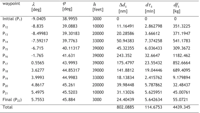
![Table 5-5: List of waypoints in 1st trajectory of medium haul flight waypoint [deg] [deg] h [feet] d k [nm] d k [min] df k [kg] Initial (P 1 ) -9.0405 38.9955 3000 0 0 0 P 2 -8.9373 39.1525 10000 10.63985 2.665515 1070.631 P](https://thumb-eu.123doks.com/thumbv2/123dok_br/18032957.861485/55.892.112.773.701.1122/table-list-waypoints-trajectory-medium-flight-waypoint-initial.webp)


![Table 5-10: List of waypoints in 2nd trajectory of long haul flight waypoint [deg] [deg] h [feet] d k [nm] d k [min] df k [kg] Initial (P 1 ) -9.0405 38.9955 3000 0 0 0 P 14 -9.2387 39.05683 10000 10.03791 2.514717 1010.061 P](https://thumb-eu.123doks.com/thumbv2/123dok_br/18032957.861485/59.892.107.797.140.564/table-list-waypoints-trajectory-long-flight-waypoint-initial.webp)