Broadband matched-field tomography using simplified acoustic systems

(1)

Universidade do Algarve

Faculdade de Ciˆ

encias e Tecnologia

Broadband Matched-Field Tomography

using simplified Acoustic Systems

(Tese para a obten¸cão do grau de Doutor no ramo de Engenharia Electrónica e Computa¸cão, especialidade de Processamento de Sinal.)

Cristiano Soares

Orientador: Doutor S´ergio Manuel Machado Jesus, Professor Associado da Faculdade de Ciˆencias e Tecnologia, Universidade do Algarve

Constitui¸c˜ao do J´uri:

Presidente: Doutora Maria da Concei¸cão Abreu e Silva, Professora Catedrática da Faculdade de Ciências e Tecnologia, Universidade do Algarve.

Vogais: Doutora Eliza Michalopoulou, Professora da New Jersey Institute of Technology, University Heights, EUA;

Doutor Victor Alberto Neves Barroso, Professor Catedrático do Instituto Superior Técnico da Universidade Técnica de Lisboa;

Doutor S´ergio Manuel Machado Jesus, Professor Associado da Faculdade de Ciˆencias e Tecnologia, Universidade do Algarve;

Doutora Maria da Gra¸ca Cristo dos Santos Lopes Ruano, Professora Associada com Agrega¸c˜ao da Faculdade de Ciˆencias e Tecnologia, Universidade do Algarve;

Doutor José Manuel Bioucas Dias, Professor Auxiliar do Instituto Superior Técnico da Universidade Técnica de Lisboa;

Doutor Paulo Alexandre da Silva Felisberto, Professor Adjunto da Escola Superior de Tecnologia da Universidade do Algarve;

Doutora Maria Jo˜ao Torres Dolores Rendas, Investigadora do Centre Nacional de la Recherche Scientifique, Fran¸ca.

Faro 2007

(2)

(3)

Universidade do Algarve

Faculdade de Ciˆencias e Tecnologia LABorat´orio de Processamento de Sinal

Broadband Matched-Field Tomography

using simplified Acoustic Systems

(Tese para a obten¸cão do grau de Doutor no ramo de Engenharia Electrónica e Computa¸cão, especialidade de Processamento de Sinal.)

Cristiano Soares

Orientador: Doutor Sérgio Manuel Machado Jesus, Professor Associado da Faculdade de Ciências e Tecnologia, Universidade do Algarve Constitui¸cão do Júri:

Presidente: Doutora Maria da Concei¸cão Abreu e Silva, Professora Catedrática da Faculdade de Ciências e Tecnologia, Universidade do Algarve.

Vogais: Doutora Eliza Michalopoulou, Professora da New Jersey

Institute of Technology, University Heights, EUA;

Doutor Victor Alberto Neves Barroso, Professor Catedrático do Instituto Superior Técnico da Universidade Técnica de Lisboa; Doutor Sérgio Manuel Machado Jesus, Professor Associado da Faculdade de Ciências e Tecnologia, Universidade do Algarve; Doutora Maria da Gra¸ca Cristo dos Santos Lopes Ruano, Professora Associada com Agrega¸cão da Faculdade de Ciências e Tecnologia, Universidade do Algarve;

Doutor José Manuel Bioucas Dias, Professor Auxiliar do Instituto Superior Técnico da Universidade Técnica de Lisboa; Doutor Paulo Alexandre da Silva Felisberto, Professor Adjunto da Escola Superior de Tecnologia da Universidade do Algarve;

Doutora Maria Jo˜ao Torres Dolores Rendas, Investigadora do Centre Nacional de la Recherche Scientifique, Fran¸ca.

Faro 2007

(4)

(5)

I

`

A Telma,

ao pequenino Guilherme, e aos meus pais.

(6)

(7)

III

Acknowledgements

I would like to thank my supervisor Prof. S´ergio M. Jesus for his permanent effort in providing the necessary conditions in the labo-ratory for accomplishing the objectives of this work, by organizing scientific projects and sea trials for collecting experimental data, his useful advises, and in particular, for his contributions through many suggestions and comments during the writing of this thesis. I thank also my colleagues in the Signal Processing Labora-tory that daily contributed for an enjoyable social environment. Finally, special thanks to my wife, for her patience and sup-port, specially during the writing of this thesis.

The financial support was given by the Funda¸c˜ao para a Ciˆencia e Tecnologia under the ATOMS project (contract PD-CTM/P/MAR/15296/1999) and a doctoral fellowship (contract SFRH/BD/12656/2003).

(8)

(9)

V Name: Cristiano Jos´e da Palma Soares

College: Faculdade de Ciˆencias e Tecnologia University: Universidade do Algarve

Supervisor: Doutor S´ergio Manuel Machado Jesus, Professor Associado da Faculdade de Ciˆencias e Tecnologia, Universidade do Algarve Thesis title: Broadband Matched-Field Tomography using simplified Acoustic

Systems

Abstract

Ocean Acoustic Tomography is a remote sensing technique that has been proposed to infer physical properties of the ocean traversed by the sound field. Although its feasibility has been demonstrated, it is still not being used in a systematic way due, in a large extent, to cost and operational difficulties of standard acoustic systems. Current developments of acoustic systems go in the sense of simpli-fying them, both at the emitting and receiving end. Simplisimpli-fying an acoustic system may represent a loss or a reduction of the amount of information contained in the observed acoustic field, possibly conducting to degradation in the inversion results. The objective of this thesis is to adapt existing array processing methods to be used in acoustic tomography and geoacoustic inversion taking into account the challenges posed by such simplifications, and to cope with the loss of available information they may represent. Two as-pects are exploited with the objective of coping with the reduction of information: one is the development of a broadband data model, and the other is the development of matched-field processors based on that broadband data model, with particular emphasis in high-resolution processors. Matched-field based approaches appear to be suitable to work in conjunction with the simplified acoustic sys-tems used to collect several experimental data sets treated herein. Experimental results using simplified acoustic systems, sparse re-ceiving arrays (active mode) on one hand, or an uncontrolled source (passive mode) on the other hand, show that it is possible to pro-duce environmental estimates of the watercolumn and seafloor in close agreement with ground truth measurements.

Key-words: Acoustic tomography, simplified acoustic systems, broadband, environmental estimation, coherent processing, high-resolution.

(10)

(11)

VII Nome: Cristiano Jos´e da Palma Soares

Faculdade: Faculdade de Ciˆencias e Tecnologia Universidade: Universidade do Algarve

Orientador: Doutor S´ergio Manuel Machado Jesus, Professor Associado da Faculdade de Ciˆencias e Tecnologia, Universidade do Algarve T´ıtulo da Tese: Tomografia por Ajuste de Campo em Banda-Larga utilizando

Sis-temas Ac´usticos simplificados

Resumo

A Tomografia Acústica Oceânica é uma técnica de medida re-mota que foi proposta para inferir acerca das propriedades f´ısicas do oceano atravessado pelo campo acústico. Embora tenha sido demonstrado que esta técnica é praticável, a mesma não é ainda utilizada de forma sistemática, em larga medida, devido aos cus-tos e dificuldades operacionais dos sistemas acústicos tradicionais. Os desenvolvimentos actuais de sistemas acústicos vão no sentido da sua simplifica¸cão, quer do lado da emissão, quer do lado da recep¸cão. A simplifica¸cão de um sistema acústico poderá repre-sentar uma perda ou uma redu¸cão da quantidade de informa¸cão contida no campo acústico observado, conduzindo possivelmente a uma degrada¸cão nos resultados de inversão. O objectivo desta tese é adaptar métodos de processamento de antenas existentes, de forma a serem utilizados em tomografia acústica e inversões geoacústicas, tomando em considera¸cão os desafios colocados por tais simplifica¸cões, e combater a perda de informa¸cão dispon´ıvel que as mesmas representam. Dois aspectos são explorados com o objectivo de combater a redu¸cão de informa¸cão: um é o desenvolvi-mento de um modelo de dados de banda larga, e o outro é o de-senvolvimento de processdores por ajuste de campo baseados nesse modelo de dados, com particular ênfase nos processadores de alta resolu¸cão. Os métodos por ajuste de campo parecem ser apropria-dos para trabalhar em conjun¸cão com os sistemas acústicos simpli-ficados utilizados para adquirir os vários conjuntos de dados experi-mentais tratados neste trabalho. Resultados experiexperi-mentais obtidos com sistemas acústicos simplificados, com antenas de recep¸cão es-parsas (modo activo) por um lado, e com uma fonte não-controlada (modo passivo) por outro, mostram que é poss´ıvel produzir estima-tivas ambientais da coluna de água e do fundo oceânico de acordo com medidas in-situ.

Palavras-chave: Tomografia acústica, sistemas acústicos simplifi-cados, banda-larga, estima¸cão ambiental, processamento coerente, alta resolu¸cão.

(12)

(13)

List of Figures

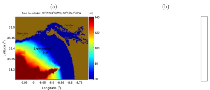
2.1 Temperature profiles and respective EOFs measured at several places: Por-tuguese West coast near Set´ubal in October 2000 ((a) and (d)); North Elba Island area in June 2003 ((b) and (e)); Portuguese West coast near Set´ubal in April 2004 ((c) and (f)). . . 16 2.2 Bathymetry maps corresponding to the experimental sites of the: INTIFANTE’00

and MREA’04 sea trials (a); MREA’03 (b). . . 22 2.3 Factors of difficulty for a global search algorithm: Multi-modality (a); isolation

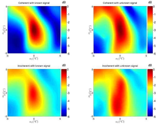
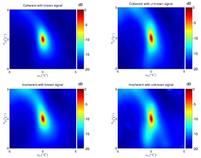
(b). . . 29 5.1 The behavior of the broadband Bartlett processor for the coherent case (upper

row); incoherent case (lower row); known signal (left column); and unknown signal (right column). . . 75 5.2 The behavior of the broadband MV processor for the coherent case (upper

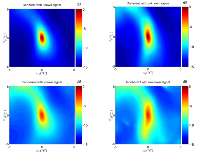
row); incoherent case (lower row); known signal (left column); and unknown signal (right column). . . 77 5.3 The behavior of the broadband MUSIC processor for the coherent case (upper

row); incoherent case (lower row); known signal (left column); and unknown (right column). . . 78 5.4 2-dimensional histograms showing the dispersion of the estimates of the

pa-rameter vector [α1α2]T: N = 9 in the left column; N = 45 in the right

column. . . 80 5.5 Eigenspectra for finite number of signal observations: comparison of two

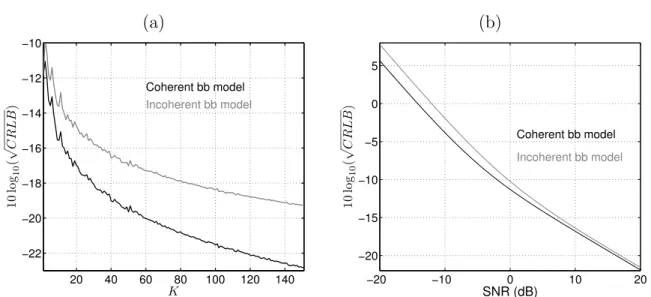
eigen-spectra using N = 9 (gray) and N = 11 black (a); average eigenspectrum for a varying number of signal realizations (b); average order estimation for a varying number of signal realizations (c). . . 83 5.6 The Cram´er-Rao Lower Bounds computed for coherent and incoherent data

models: (a) CRLB as a function of K, the number of equispaced frequency bins in the band 900-1200 Hz; (b) CRLB as a function of SNR using frequen-cies 400, 450, and 500 Hz. . . 84 5.7 The RMSE for the three processors and the coherent model CRLB under

comparison: (a) RMSE as a function of SNR with known signal matrix; (b) RMSE as a function of SNR with unknown signal matrix; (c) RMSE as a function of N with known signal matrix; (d) RMSE as a function of N with unknown signal matrix. . . 85 5.8 Ambiguity surfaces against α1 and α2 computed using cross-frequencies. . . . 87

5.9 Signal matrix estimates obtained from synthetic data considering increasing source displacement during the observation interval. . . 89

(16)

XII

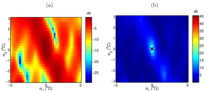
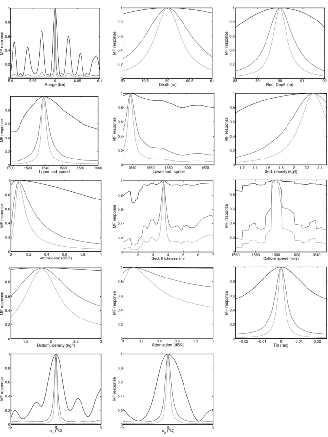
5.10 Comparison of standard computation of cross-frequency SDM (left column) and computation with phase normalization (right column): cross-frequency SDMs ((a) and (b)); eigenspectra ((c) and (d)); application with Bartlett processor ((e) and (f)). . . 91 5.11 Sensitivity of the processors to the channel parameters: BB Bartlett (black);

BB MV (darkgray); BB MUSIC (lightgray). The processors are all coherent with known signal matrix. . . 93 5.12 RMSE obtained during inversions with GA for the different parameters

com-bining the three processors with three values of the number of signal realiza-tions. A white asterisk indicates the processor with lowest RMSE for that number of signal realizations. . . 95 5.13 A posteriori probability distributions for each parameter based on the last

generation of 20 independent populations. Each column respects to each of the processors entering the comparison. The gray asterisks indicate the correct parameter value. . . 97 6.1 GPS estimated AOB and source ship navigation during the deployment of

June 21st. . . 104 6.2 Source range (a) and depth (b) measured during the deployment of June 21st. 104 6.3 Baseline model for the MREA’03 sea trial. All parameters except waterdepth

are range-independent. . . 106 6.4 Observations of phases over time for receivers 1 to 3 at frequencies 910, 964,

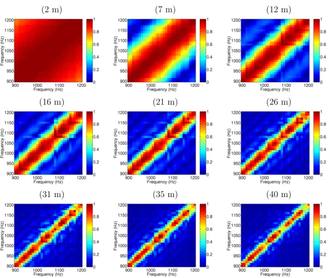
1017, and 1071 Hz. . . 107 6.5 Diagonal normalized cross-frequency SDMs obtained for different source ranges

and speeds (see table 6.2). . . 108 6.6 Resulting phases after applying phase normalization over time for receivers 1

to 3 at frequencies 910, 964, 1017, and 1071 Hz. The receiver with constant value of 0 is the reference receiver. . . 110 6.7 Cross-frequency SDMs with phase normalization obtained for different source

ranges and speeds (see table 6.2). . . 110 6.8 Histograms showing how the components of the optimized frequency vector

are distributed. . . 112 6.9 Source localization as a MFT validation step. Source range (left column) and

source depth (right column). True location is given by the red curve in the background. The gray curve with circles are the source localization results. The black asterisks indicate the successful localizations. . . 116 6.10 Model parameters estimates obtained via MFT using the BB MUSIC

proces-sor. Water column ((a)-(b)); sediment ((c)-(g)); sub-bottom ((h)-(j)); geomet-ric ((k)-(l)); MF response ((m)). The black asterisks indicate model estimates allowing for successful source localization in the validation step. . . 119 6.11 A posteriori probability distributions for the seafloor parameters based on

the last generation of the GA. Only inversions validated by means of source localization during the A2 period are considered. The gray asterisk indicates the baseline value of the parameter. . . 120 6.12 Reconstruction of the temperature profiles estimated using the BB MUSIC

processor. Only profiles corresponding to successful source localization are taken into consideration (see figures 6.10(a) and (b)). The gaps in between were filled by linear interpolation in time. . . 122

(17)

XIII

7.1 GPS estimated AOB and source ship navigation during the deployment of April 8. . . 128 7.2 Source range (a) and depth (b) measured during the deployment of April 8. . 129 7.3 Baseline model for the MREA’04 sea trial. All parameters except waterdepth

are range-independent. . . 131 7.4 Model parameters estimates obtained via MFT using the BB MUSIC

proces-sor. Water column ((a)); sediment ((b)-(f)); sub-bottom ((g)-(i)); geometric ((j)-(k)); MF response ((l)). The black asterisks indicate model estimates allowing for successful source localization in the validation step. . . 136 7.5 Reconstruction of the temperature profiles estimated using the BB MUSIC

processor with K = 6. Only profiles corresponding to successful source local-ization are taken into consideration (see figures 7.4(a)). The gaps in between were filled by linear interpolation in time. . . 137 8.1 INTIFANTE’00 sea trial: acoustic runs and bathymetry during Events 2, 5

and 6, X signs mark the XBT locations and VLA indicates the vertical line array location. . . 144 8.2 GPS estimated ship speed (a) and ship heading (b) during Event 6 . . . 144 8.3 NRP D. Carlos I ship radiated noise received on hydrophone 8, relative power

scale on a time-frequency plot (a) and mean power spectrum (b). . . 145 8.4 Range-independent baseline model for the INTIFANTE’00 sea trial. . . 146 8.5 Examples of phases measured during Event 6 at frequencies 359 and 718 Hz. 148 8.6 INTIFANTE’00 sea trial, Event 6 frequency selection: 1 selection and 0

-no selection based on contiguous snapshot mean signal coherence along time (eq. (8.1)). . . 149 8.7 Focalization results for Event 6: Bartlett power (a), source range (b)[the

continuous line is the GPS measured source-receiver range], source depth (c), receiver depth (d), sediment compressional speed (e), sediment thickness (f), sub-bottom compressional speed (g), VLA tilt (h), EOF coefficient α1(i), EOF

coefficient α2 (j) [filled dotted lines are the XBT measured data projected onto

the respective EOFs] and reconstructed temperature (k). . . 150 8.8 INTIFANTE’00 sea trial, Event 6: histograms of the EOF coefficients

esti-mates for α1 (a) and α2 (b). . . 152

(18)

(19)

List of Tables

2.1 Minimum and maximum values of the mean profile considered at each sea trial. 17 5.1 Peak-to-surface average ratio obtained for the different processors. Coh. and

Inc. respectively stand for coherent and incoherent. k. and unk. respectively stand for known signal and unknown signal. . . 79 5.2 Variances of the estimates of α1 and α2 obtained with the three proposed

processors applied to synthetic data (see figure 5.4). . . 81 5.3 Number of parameters in which a processor obtained lowest RMSE for a given

number of signal realizations (see figure 5.12). . . 96 6.1 Signal emission schedule during June 21st. The times are in GMT. . . 105 6.2 Times, source ranges and source speeds respective to the plots in figure 6.5. . 109 6.3 GA forward model parameters with search bounds and quantization steps for

MFT. . . 114 6.4 GA settings for MFT. . . 114 6.5 Rates of successful localization for the different processors and different signals.117 6.6 Baseline seafloor parameters, two parameter distributions based on 43 GA

populations, and a reliability measure. . . 121 7.1 GA forward model parameters with search bounds and quantization steps for

MFT. . . 132 7.2 Standard deviations of the parameter estimates as the number of frequencies

K increases. In the bottom line source localization rate. . . 134 7.3 Comparing standard deviations of the parameter estimates at all times (a)

with standard deviations considering only times on successful source localiza-tion (validalocaliza-tion step) (b). . . 135

(20)

(21)

Chapter 1 Introduction

Generalities and work motivation

The propagation of sound in the ocean is strongly influenced by the environmental conditions. The sound field is sensitive to the propagation velocity which depends on the geophysical properties of the watercolumn and seafloor. The interaction of the propagating sound with the seafloor is particularly relevant in shallow-water (less than 200 m) as it is reflected at the seafloor and transmitted into the sediments. Being able to predict the acoustic behavior of a given environment is the key to current advances in the usage of acoustics for ocean exploration [1]. This implies that, for example, the sonar detection of a sound source in range and depth depends on the environmental knowledge of a given propagation scenario. Conversely, the interaction between sound waves and the environment allows for retrieving environmental information from the analysis of the emitted and received signals. Acoustic ocean exploration is an appealing complement to classical ocean exploration.

Classical ocean exploration is based on direct measurements of physical quantities of the ocean. Direct in-situ measurements of the physical quantities in the watercolumn or in the seafloor are usually time consuming, very expensive and offer poor spatial coverage. In other words, direct methods are generally slow and the regions that can be covered are

(22)

2 CHAPTER 1. INTRODUCTION

small compared to the size of the ocean. Moreover, direct measurements can generally not be made simultaneously at different points of the ocean, nor are they capable to show how slow physical processes vary over time or how these change with seasons or over longer time periods.

The magnitude of the ocean sampling task leads to technologies providing indirect meth-ods for assessing ocean physical quantities. These methmeth-ods clearly offer the possibility to observe physical quantities in a vast area of the ocean in a systematic way, and at lower cost than direct methods. Indirect methods consist in exploring the interaction of a wave with the media to be characterized, in order to use such interaction and its physical laws to retrieve physical quantities of interest.

An excellent example on the advantages of using indirect methods for ocean observations are satellites such as the TOPEX/Poseidon satellite that has been in service for more than 10 years [2]. This satellite covers 95% of the ice-free oceans every 10 days (!), carrying out a number of tasks such as continuously observing global ocean topography, delivering altimetric data, and observing relevant phenomena such as el Ni˜no and la Ni˜na.

However, satellites use electromagnetic waves, which are strongly attenuated by sea water and are therefore essentially suitable for observing the ocean surface. Acoustic waves, on the other hand, propagate well in the ocean, providing means to remotely sense the interior of it, using the generic advantages of indirect methods for assessing its physical properties. There are examples of acoustic applications that have been commercially available for several years. The Acoustic Doppler Current Profiler (ADCP), an acoustic device that attempts to produce a record of water current velocities over a range of depths, is now considered an indispensable aid for oceanography, estuary, river and stream flow current measurement.

(23)

3

The side-scan sonar is used for mapping the seabed for a wide variety of purposes such as identification of bathymetric features and understanding material and texture type of the seabed.

One of the most relevant physical properties is the temperature in the watercolumn. Ocean Acoustic Tomography is a remote sensing technique that has originally been proposed to infer this physical property. Although its feasibility has been demonstrated and despite the advantages of this technique, it is still not being used in a systematic way. This concept requires expensive acoustic emitting and receiving equipment to be maintained and operated at several locations in order to obtain sufficient source-receiver propagation paths to cover a given ocean volume. Installing acoustic systems on a long-term or permanent basis may become problematic, since some areas of interest are just not suitable for that. In practice, many acoustic systems operate at low frequencies, implying the use of bulky and expensive sound projectors and large aperture receiving arrays. Operational difficulties arise due to the deployment requirements of those equipments. Most of the acoustic apparatus used today in acoustic tomography are still prototypes and research oriented. From a completely different point of view, biologists and environmentalists have demonstrated concerns on how sound transmissions across the ocean affect marine mammals.

In order to alliviate these problems faced by the sound technology used in ocean acoustic tomography one can operate simplifications either on the emitting end, or on the receiving end of the acoustic system. The simplification of one end of the acoustic system has perhaps to be accompanied by an increase of complexity on the other end in order to prevent a decrease of performance of the whole system. Simplifications on the receiving end can be operated by reducing the number of receivers typically used, and/or by reducing the array

(24)

aperture. It is also possible to design a receiving system such that it can be deployed in a free-drifting configuration instead of a moored configuration. Operating these simplifications, one at a time or all together, will essentially reduce the size of those receiving equipments and their deployment requirements. At the emitting end one can reduce the size of the emitting source, which would reduce the deployment requirements, at the cost of an increase of the emitting frequencies. Another possibility is to completely eliminate the source, taking advantage of the fact that the marine environment is naturally noisy, specially due to animal or human activity, and surface hydrodynamic phenomena. Thus, the idea of using sources of opportunity that are naturally present is an appealing alternative to a controlled source in areas where deploying a permanent controlled source is impossible or too costly, in the presence of marine mammals, or for covert military applications.

The characteristics enumerated above, represent a reduction in the complexity of acoustic systems used in acoustic tomography, in comparison to standard acoustic systems. Such reduction in complexity is, in principle, obtained at the cost of a reduction of available information in the observed acoustic field. The objective of the work presented in this thesis is to extend existing or propose new signal processing methods being able to exploit simple and handy acoustic systems for ocean acoustic tomography. The implications and challenges of using such acoustic systems in acoustic tomography have to be identified, in order to understand which observables of the acoustic propagation can be used, together with the field inversion algorithm to be applied.

Ocean acoustic tomography: background

In 1979 Munk and Wunsch [3, 4] proposed Ocean Acoustic Tomography (OAT) as a concept for global ocean monitoring. OAT can be defined as the cross-sectional imaging of a region

(25)

5

from either transmitted or reflected pressure fields collected when insonifying the region from different directions. The problem of Ocean Acoustic Tomography is to infer from precise measurements of travel time, or other properties of acoustic propagation, the state of the ocean traversed by the sound field. The rationale behind that concept is that the ocean is largely transparent to sound, and that sound travel time depends on the temperature (and to a much lesser extent, on salinity). Conversely, measurements of the time that acoustic energy takes to travel from emitter to receiver can provide information about the intervening ocean using inverse methods.

At the same time Matched-Field Processing (MFP) was being proposed for source local-ization problems [5, 6]. MFP is a full-field signal processing method that takes advantage of the spatial properties of the acoustic field and the knowledge of the ocean properties between source and receiver to retrieve source location (see [7] and references herein). A measured field is compared to model replicas calculated for hypothetical source positions within a specific range and depth search region to form an ambiguity surface whose maxi-mum will indicate the location of the acoustic source provided that the underlying physical model is sufficiently accurate. The comparison between the field and the replicas is done by means of a processor which usually is a correlation function based on statistical assumptions made on signal and noise. Since the acoustic signal is used as an intermediate observable to estimate source location, MFP can be considered to be an inverse problem. However, the calculation of the replica signal is more difficult than in conventional array processing since it involves solving the wave equation on the actual physical scenario. The knowledge on the parameters of the actual physical scenario is of paramount importance in MFP based processing approaches, since the ability to predict the acoustic behavior of this scenario,

(26)

and consequently the source location estimation performance will depend on those physical parameters. Hinich [5] was the first to examine source localization with a vertical array, but Bucker [6] is credited to be the first to formulate MFP, as he used realistic environmen-tal models, introduced the concept of ambiguity surface and demonstrated that there was enough complexity of the wave field to allow inversion - localization.

From the algorithmic point of view, there are essentially two types of algorithms for performing ocean acoustic tomography. One is the original concept, by Munk and Wunsch, and is based on the travel times of the sound through multiple paths, and has been termed Travel-Time Tomography (TTT) [3]. The other is Matched-Field Tomography (MFT), which is similar to the Matched-Field Processing (MFP) technique, except that the source location is known, and parameters of the intervening ocean are to be estimated [8, 9, 10, 11]. TTT makes direct use of the multipath nature of the sound propagation in the ocean. One looks for the perturbations of the sound-speed around a background value instead of the sound-speed profile itself. The modeled travel times are calculated taking advantage of linearizable equations making direct inversion possible. This approach was initially proposed for deep water regions where the ray approximation was valid and sound speed could be analytically linked to acoustic ray time [4]. Since it uses absolute times, travel-time based tomography turned out to be highly dependent on the ability to separate closely spaced arrivals and the precise knowledge on the source-receiver relative position at all times. Moreover, it appears to be limited to tomographic problems where the linearization approach is applicable. In shallow-water, TTT suffers degradation due to arrivals that can not be identified or separated. On the other hand, in shallow-water, there is the need to infer seafloor properties, about which little or no information is contained in the travel times.

(27)

7

Instead, MFT is applicable to problems where one looks for the actual value of the parameters rather than their perturbations around a background value. In that case the problem is highly non-linear and a linearization approach is no longer a realistic option. As direct inversion is not possible, the inversion is posed as an optimization problem in an attempt to maximize the match between the measured acoustic field and the replica field calculated for candidate parameter values. Several authors have used this technique for performing geoacoustic inversions of field data [12, 13, 14, 15, 16].

MFT is often applied in shallow water scenarios where the seafloor parameters have an important influence on the field propagation. The seafloor parameters are often unknown, and have therefore to be estimated together with the parameters of the watercolumn. This arises one of the hardest problems to deal with, in MFT, which is the high number of un-knowns that may enter the inverse problem. The inverse problem is in general ill-conditioned and the parameter space is usually very large. Thus, there is the inherent risk that the fi-nal model estimate may represent an acoustically equivalent but environmentally different model from the true model, leading to erroneous environmental parameter estimates. This problem leads to another important discussion in MF approaches, which is on the ability of the processor to reject sidelobes. In the past much effort has gone into developing processor techniques to suppress sidelobes as much as possible. This issue is particularly important in inverse problems where many parameters are left as unknowns. Depending on the param-eters in play, the specific physics of the scenario at hand, and the geometric setup of the experiment, complicated ambiguity patterns might be generated. The ability of discriminat-ing closely spaced acoustic fields depends on the degree of uniqueness of the acoustic pressure field. This can be achieved by using a high number of receivers or eventually by employing

(28)

high-resolution methods as discussed by Collins et al. [17]. Examples of high-resolution methods are matched-field processors derived from the concepts of minimum-variance [18] or subspaces [19]. These methods offer significantly higher sidelobe attenuation in compar-ison to Bartlett-like methods and usually involve comparcompar-isons beyond simple correlations. However, there have been a reduced number of papers applying either the minimum-variance processor [20, 21], or subspace based methods [22] to real acoustic data with some degree of success.

Ocean acoustic tomography using simplified acoustic systems

Ocean acoustic tomography experiments in deep water regions for large-scale ocean moni-toring have used multiple sources and multiple arrays in order to determine the variability of the three-dimensional water temperature field [23, 24, 25]. In shallow-water tomography experiments the simple configuration of a single source and a single vertical array of receivers has been used in several occasions. The acoustic source is usually towed by a research vessel, in order to cover a certain area of interest, and the receiving array traditionally employed has a high number of hydrophones (see e.g. [13, 14, 16]) in order to sufficiently sample higher order normal modes and assure as much as possible uniqueness in the problem solution.

Current developments of receiver systems go in the sense of reducing their overall size along with the length of the array itself and the number of receivers with the objective of reducing the cost and deployment requirements of these systems. This means that the acoustic field will be heavily undersampled representing therefore an additional challenge in terms of conditioning of the inverse problem. The other simplification already mentioned, the free-drifting deployment of the receiver array, poses a challenge in terms of knowledge of the position of the receiving array. A number of papers using sparse vertical arrays exist.

(29)

9

Siderius et al. [15] used 4-hydrophone arrays distributed over a range of 40 km to invert range-dependent bottom properties from broadband transmission loss in the frequency band 200-800 Hz. Felisberto et al. [26] demonstrated with experimental data that successful inversions for the watercolumn in shallow water can be obtained with a 4-hydrophone vertical array using a known broadband source with a bandwidth of 700 Hz about 10 km away from the vertical array. Here an arrival matching processor was used. Le Gac et al. [27] developed a geoacoustic inversion process based on the use of a model-based matched-impulse response using broadband acoustical signals on a single hydrophone. The methods used in all these studies involve the correlation of the received signals with the emitted signal to estimate the channel impulse response, and therefore require broadband signals. More recently Soares et al. have obtained tomography inversion results using sparse vertical line arrays with 4 elements [28, 29] and with 3 elements [30, 31]. All results were obtained with cross-frequency MF processors without using knowledge of the emitted waveform. In Refs. [30, 31] high-resolution processors were used.

From the emitter point of view it can be said that the majority of acoustic tomography studies used controlled acoustic sources and therefore fall in the case of active tomography. In opposition, Passive Acoustic Tomography (PAT), a variant of acoustic tomography where the usual controlled source is replaced by a source of opportunity, represents a significant increase of the complexity of the inverse problem in comparison to active tomography. Using a source of opportunity will in principle lead to a loss of signal-to-noise ratio of the received signals. As the emitted waveform is unknown, the extraction of observables as for example travel-times or ray amplitudes of acoustic rays is strongly degradated in terms of accuracy. In that way, travel-times and ray amplitudes in PAT are relative to those of the first arrival,

(30)

and no longer absolute quantities as in active tomography. Further attributes of the emitted signal are that it may contain stochastic components, and the signal may suffer fluctua-tions during the observation time both in strength and bandwidth. Also the position of the source may be unknown and changing over time, and may therefore constitute a nuisance parameter to be added to the parameters of interest to be estimated from received acoustic fields. Furthermore, not knowing the source position implies that other propagation chan-nel characteristics such as waterdepth or seafloor properties are also unknown and must be estimated. There is a generic approach in signal processing called blind system identifica-tion for estimating the input signal or system parameters when only the output data are known. A passive acoustic tomography problem with unknown emitted signal and unknown channel properties can be termed blind ocean acoustic tomography (BOAT). The distinction between PAT and BOAT is that the former aims at estimating ocean temperature with al-ternative passive sources, while the latter produces a full environmental estimate, including water column, bottom properties, and source-receiver geometry as well as a source-emitted power spectrum, without any knowledge or control on the acoustic illuminating source. The tomographic problem suffers significant increase both in complexity and uncertainty when one passes from active mode to passive mode.

A number of papers reporting the idea of using alternative illuminating sources for OAT and geoacoustic inversion exist. Two groups of applications for inferring ocean properties have been proposed in the literature. One uses ship radiated noise and vocalizations of marine mammals for watercolumn or geoacoustic inversion. The other uses surface generated noise for geoacoustic inversion. Chapman [32] describes an approach for geoacoustic inversion using ship noise data collected with a 16-hydrophone vertical line array. Ship noise data

(31)

11

were recorded as a ship followed an arc segment at a range of 3.3 km from the array. Jesus et al. [33, 34] applied MFT on ship noise data of a research vessel describing arcs of 1.2, 2.2, and 3.2 km recorded on a 16-hydrophone vertical line array. Thode et al. [35] performed global inversions using blue whale vocalizations from 8 elements of a vertical line array to extract information on bottom composition, array shape, and the animal’s position. Other authors used ship-towed horizontal arrays recording the noise emitted by the towing-ship itself or by a cooperative ship to estimate ocean parameters [36, 37, 38]. All these studies except [38] used MFP based inversion methods.

Concerning the applications using surface generated noise Buckingham first proposed to use acoustic daylight to form images of silent objects in the ocean [39, 40] and then using ambient noise for geoacoustic inversion [41]. More recently Harrison [42, 43, 44] used sea surface wind induced noise and then Buckingham et al. [45] used light aircraft air induced noise, both with the purpose of shallow water geoacoustic inversion.

The simplifications that can be operated in an acoustic system, at the emitting end or at the receiving end, discussed in this chapter basically imply that the amount of information available in the received acoustic field is reduced in comparison to that when a traditional acoustic system is used to emit and receive signals. At the emitting end, using a source of opportunity, such as for example ships or marine mammals, corresponds to a loss of control on one hand, and to a lack of knowledge on emitted waveform on the other hand. On the receiving end, the reduction of available information is essentially a consequence of the sparsity of the receiver elements.

This thesis deals with this important implication by proposing MFP based array pro-cessing methods that attempt to cope with the increased ill-conditioning of the underlying

(32)

inverse problem by extracting more information from the acoustic signals than conventional processing. The algorithms developed in this thesis can be applied for estimating watercol-umn, bottom properties, and source position.

Organization of this thesis

This thesis is organized as follows: chapter 2 briefly reviews some fundamental topics such as the dependence of sound-speed, sound-propagation, and inverse problems in MFP. Chapter 3 develops a broadband data model and discusses some related aspects. Chapter 4 develops three matched-field processors based on the broadband data model: the Bartlett processor, the minimum-variance processor, and the MUSIC processor. Chapter 5 reports a series of computer simulations performed for numerically characterizing and comparing the three pro-cessors. Chapter 6 reports experimental results on MFT applied to the MREA’03 data set comparing the three processors developed. Chapter 7 reports experimental results on MFT applied to the MREA’04 data set testing the performance of a high-resolution processor with a varying number of frequencies and a scheme for validating environmental inversions. Chapter 8 reports experimental results on passive acoustic tomography applied to the IN-TIFANTE’00 data set. Finally, chapter 9 draws conclusions on the achievements of this thesis and gives suggestions for future work.

(33)

Chapter 2 Theoretical background

The present chapter reviews several concepts used in the remaining text of this thesis. This chapter is broadly divided into two groups of subjects. One is on the underlying physics of the problem by treating concepts such as the sound-speed in the ocean, the modeling of sound propagation in the ocean, and modeling of sound propagation in range-dependent environments (sections 2.1, 2.2, 2.3). The other deals with the inverse problem, by review-ing environmental focalization, an inversion technique based on Matched-Field Processreview-ing (section 2.4); and genetic algorithms which is a global search method used in focalization problems (section 2.5).

2.1 The sound-speed

The sound speed in the ocean plays a fundamental role in sound propagation. Through the times the sound speed has been related to physical and chemical parameters, but it can simply be seen as an increasing function of temperature, salinity, and pressure. A simplified expression for this dependence is the Mackenzie formula [46, 47], given as

c(T, z, S) = 1449.2 + 4.6T − 0.055T2+ 0.00029T3+ (1.34 − 0.01T)(S − 35) + 0.016z, (2.1) 13

(34)

14 CHAPTER 2. THEORETICAL BACKGROUND

where c is the sound speed in m/s, T is the temperature in ◦C, z is depth in m, and S is salinity in ppt. It can be seen that in shallow water the temperature has the most important contribution for the sound speed. In deep water, and for large depths, the last term containing depth z dominates the sound speed. The speed of sound in the ocean shows only small departures from 1500 m/s, usually less than 1%. Nevertheless the effect of small variations of the sound speed on sound propagation in the ocean is profound.

For estimating the ocean sound speed profile via acoustic tomography, the direct estima-tion of the sound speed profile is the simplest approach as it directly reflects the parameters required. However, in general a sound speed profile contains a large number of data points - thus, direct estimation of those data points could be cumbersome. The ocean sound speed can be efficiently represented via shape functions. Empirical orthogonal functions (EOF) have extensively been used for ocean sound speed estimation. EOFs are orthogonal shape function [48] that can be obtained from a database and are very efficient to reduce the number of data points. If historical data is available, an efficient parameterization in terms of EOFs leads to faster convergence and higher uniqueness in the optimal solution since a great deal of information is included and the search is therefore started close to the solution, besides representing a way of strongly constraining the solutions that can be obtained [8]. For this purpose, for example, EOFs are constructed from representative data by sampling the depth dependence of the ocean temperature. The EOFs are obtained by computing the singular value decomposition (SVD) of a matrix CTT with columns

[CTT]i = Ti− ¯T, (2.2)

(35)

2.1. THE SOUND-SPEED 15

to be

CTT = UDV, (2.3)

where D is a diagonal matrix with the singular values, and U is a matrix with orthogonal columns, which are used as the EOFs. The temperature profile is obtained by

ˆ T_EOF = ¯T + N X n=1 αnUn, (2.4)

where αn is a coefficient associated to the EOF Un, and N is the number of EOFs to be

combined, which is selected by observation of the singular values by using some empirical criterion. The criterion used in this study to select the number of relevant EOFs for the available data is ˆ N = min N PN n=1λ2n PM m=1λ2m > 0.8, (2.5)

where the λn are the singular values obtained by the SVD, and λ1 ≥ λ2 ≥ . . . ≥ λM. M

is the total number of singular values. Experimental results have shown that usually the first 1, 2 or 3 EOFs are enough to achieve a high degree of accuracy. The use of EOFs involves historical data that in the case of the water column temperature profile can be acquired over time and space. Thus, one can expect to have sufficient information to enable the model to obtain the profile that best represents the watercolumn over range, depth and time. Figure 2.1 shows temperature profiles measured during several sea trials with the respective EOFs obtained via SVD. They were obtained during different seasons of the year at different places, which can clearly be seen to have a strong influence on their shapes. The temperature and depth scale is the same on all plots for the sake of easy comparison. Figure 2.1(a) shows the profiles measured with XBTs during the INTIFANTE’00 sea trial, which took place off the Portuguese West coast near Set´ubal in October 2000 [49]. The mean profile varies 3.6◦C between the top and the bottom. Table 2.1 shows the minimum and

(36)

16 CHAPTER 2. THEORETICAL BACKGROUND (a) (b) (c) 14 16 18 20 22 24 26 0 20 40 60 80 100 120 Temperature (oC) Depth (m) Mean temperature XBT temperatures 14 16 18 20 22 24 26 0 20 40 60 80 100 120 Temperature (oC) Depth (m) Mean temperature CTD temperatures 14 16 18 20 22 24 26 0 20 40 60 80 100 120 Temperature (oC) Depth (m) Mean temperature CTD temperatures (d) (e) (f) −0.4 −0.3 −0.2 −0.1 0 0.1 0.2 0.3 0.4 0 20 40 60 80 100 120 1st_EOF 2nd_EOF Temperature (oC) Depth (m) −0.5 0 0.5 0 10 20 30 40 50 60 70 80 90 100 Temperature (o_C) Depth (m) −0.2 0 0.2 0 10 20 30 40 50 60 70 80 90 100 1st_EOF 2nd_EOF Temperature (oC) Depth (m)

Figure 2.1: Temperature profiles and respective EOFs measured at several places: Portuguese West coast near Set´ubal in October 2000 ((a) and (d)); North Elba Island area in June 2003 ((b) and (e)); Portuguese West coast near Set´ubal in April 2004 ((c) and (f)).

maximum temperatures of the average profiles considered. Figure 2.1(b) shows the profiles measured during the MREA’03 sea trial [50] which took place in the North Elba Island area in June 2003. These are typical Mediterranean Summer profiles with a strong thermocline. The variation with depth (11.5 ◦C) is clearly stronger then for those in the Atlantic Ocean. The MREA’04 took place off the Portuguese West coast near Set´ubal in April 2004 and the mean profile has a variation of 1.1◦C between the top and the bottom (figure 2.1(c)) [51]. This is a nearly isovelocity case. Winter propagation conditions are better than those in the

(37)

2.2. ACOUSTIC PROPAGATION IN SHALLOW WATER 17

INTIFANTE’00 MREA’03 MREA’04

min. 13.7 13.8 14.0

max. 17.1 25.3 15.1

Table 2.1: Minimum and maximum values of the mean profile considered at each sea trial.

Summer, since typically during summertime the temperature profile is downward refracting preventing long range propagation.

In the second row are plotted the respective EOFs obtained with the collections of mea-sured temperature profiles. Those profiles will be used for the inversion of the acoustic field in the experimental part of this study. The INTIFANTE’00 and the MREA’03 data satis-fied the criterion in equation (2.5) with the first 2 EOFs, while the MREA’04 data satissatis-fied the criterion with just the first EOF. The EOFs have interesting features that are clearly related to the variability of the measured temperatures profiles. The first EOF for the IN-TIFANTE’00 sea trial is close to zero at the top and increases with depth until a depth of 40 m, and then reduced back to zero at the bottom. The first EOF of the MREA’03 sea trial shows high variability in the first layers and then approaches to zero. Finally, the first EOF of the MREA’04 sea trial is close to zero at the top, and increases steadily with depth, indicating that some variability at deeper layers found place during the temperature measurements.

2.2 Acoustic propagation in shallow water

The wave equation in an ideal fluid can be derived from hydrodynamics and the adiabatic relation between pressure and density. Considering that the time scale of oceanographic changes is much longer than the time scale of acoustic propagation, it is assumed that the material properties density ρ and sound speed c are independent of time. The linear

(38)

approx-18 CHAPTER 2. THEORETICAL BACKGROUND

imation of the wave equation involve retaining of only first order terms in the hydrodynamic equations: ρ∇(1 ρ∇p) − 1 c2 ∂2_p ∂t2 = 0, (2.6)

where p is the acoustic pressure [1]. Note that this is a homogeneous equation, and that ρ and c2 are space dependent. Several numerical methods exist to solve this equation. The major difference between the various techniques is the mathematical manipulation of the wave equation applied before implementation of the solution. In general the task of implementing the solution of the wave equation is very difficult due to the complexity of the ocean-acoustic environment: the sound speed profile is usually non-uniform in depth and range; the sea surface is rough and time dependent; the ocean floor is typically a very complex and rough boundary which may be inclined, and its properties are usually varying over range.

Shallow water is defined as that part of the ocean lying over the Continental Shelf where the water depth is less than 200 m. At frequencies of a few hundred Hz, the shallow water column is of several wavelengths and act as a waveguide whose boundaries are the surface and the bottom. In this type of environment the acoustic field is usually represented by normal modes. The Helmholtz equation is the wave equation in the frequency domain, and can be written in cylindrical coordinates under the assumption of cylindrical symmetry as:

1 r ∂ ∂r(r ∂p ∂r) + ρ(z) ∂ ∂z( 1 ρ(z) ∂p ∂z) + ω2 c2_(z)p = − δ(r)δ(z − zs) 2πr . (2.7)

Using the technique of separation of variables the solution being searched has the form p(r, z) = Φ(r)Ψ(z). Replacing this in (2.7) and after some manipulations,

ρ(z) d dz[ 1 ρ(z) dΨm(z) dz ] + [ ω2 c2_(z)− k 2 rm]Ψm(z) = 0, (2.8)

(39)

2.2. ACOUSTIC PROPAGATION IN SHALLOW WATER 19

with k2

rm denoting the separation constant

k_rm2 = 1 Φm(r) [1 r d dr(r dΨm dr )], (2.9)

and Ψm denotes a particular function Ψ obtained with krm, and denote the modes which

build a complete set. The modal equation (2.8) is to be solved with the appropriate boundary conditions, and since the Ψm form a complete set of functions, the acoustic pressure can be

represented as p(r, z) = ∞ X m=1 Φm(r)Ψm(z). (2.10)

Thus the solution yields

p(r, z; zs) ≈ i 4ρ(zs) √ 8πre −iπ/4 ∞ X m=1 Ψm(zs)Ψm(z) eikrmr √ krm , (2.11)

where zs is the source depth. In reality the wavenumber spectrum is composed by a

contin-uous and a discrete part, corresponding to evanescent and radiating spectrum respectively. The solution in (2.11) is obtained under the assumption that the spectrum is composed only by the discrete part. Hence the solution is valid only at ranges greater or equal than several water depths away from the source.

An alternative approximation to the wave equation is the so called ”high frequency approximation” that consists in representing the acoustic field by the ray solution. The ray solution of the wave equation is a high frequency approximation, that is useful particularly for deep water problems, where generally only a few rays are significant. Ray tracing is satisfactory if the wave length is much less than the length scales in the problem. For ray tracing Snell’s law provides a simple formula for calculating the ray declination angle when the channel is modeled as a stratified medium based on the knowledge of the soundspeed at the interface between two layers. A ray connecting the emitter to the receiver is called an

(40)

eigenray. Each eigenray represents an arrival at the receiver characterized by a propagation time called arrival time given as

τ =

Z

Γ

ds

c , (2.12)

where Γ is the ray trajectory according to the Snell’s law. In reality there are multiple eigenrays connecting the source to a receiver each with a different trajectory which means that the propagation media between the emitter and the receiver is multipath, with the impulse response h(t) = T X r=1 arδ(t − τr) (2.13)

where T is the number of arrivals hitting the receiver, τr is the arrival time, and ar is the

amplitude associated to the rth _arrival.

Ray solutions can be rapidly computed, are highly intuitive and easily visualized. How-ever, diffraction effects and other low frequency behavior are not included, leading to a somewhat coarse accuracy. On the other hand, the main advantage of the normal mode method is the capability to provide highly accurate fields at reasonable computation times and at low frequencies. Since MFP is mostly applied at low frequencies in shallow water, the ray solution is rarely used. In shallow water many significant rays arrive to the receiver, whereas the modes are only a few, which further implies that mode models are preferable to ray tracing models.

2.3 Range dependent environments

In real ocean acoustic applications it is often a good approximation to consider that envi-ronmental parameters such as sound-speed profile, water depth and bottom properties are invariant with range. Range-independence can only be a simplification of the physical model

(41)

2.3. RANGE DEPENDENT ENVIRONMENTS 21

for the problem at hand since there will always be some degree of range-dependence. Com-mon examples of range-dependence are variations in the bathymetry between emitter and receiver, or variations in the water-column soundspeed caused by e.g. ocean fronts or internal tides. Oceanographic features are also variable in time and require in situ measurements to be characterized. This can be done, for example, using satellite images. Range-dependence linked to the bathymetry is easier to handle since it does not evolve with time and accurate description on the bathymetry can be obtained a priori. Figure 2.2 shows two bathymetry maps: one corresponds to the area where the INTIFANTE’00 and the MREA’04 sea trials took place which is off the Portuguese West coast near Set´ubal (Figure 2.2(a))[49, 51]; and the other corresponds to the area where the MREA’03 sea trial took place, which is the North Elba Island area (Figure 2.2(b))[50]. All these experiments provided field data propagated along tracks with range-dependent bathymetry, which throughout the present work will al-low for demonstrating that dealing with range-dependent environments is now a reality in MFP based applications. One decade ago it was not possible to perform acoustic inversions in reasonable computation times for mild range-dependence, although acoustic propagation models able to solve the forward problem for such scenarios were already available. Nowa-days this is routine. The ever decreasing price of CPU power enables a small laboratory or a small department to construct its own computer cluster, such that it is possible to process a complete data set within a day, even if range-dependent features are present.

The propagation model used in this thesis is the C-SNAP range-dependent normal modes propagation model with mode coupling [52]. If the environment is range-independent then C-SNAP implements an approximation of equation (2.11) using the M largest-order discrete modes of the problem. The numerical method employed to find the mode amplitudes is

(42)

(a) (b)

Figure 2.2: Bathymetry maps corresponding to the experimental sites of the: INTIFANTE’00 and MREA’04 sea trials (a); MREA’03 (b).

based on a widely used finite difference algorithm in combination with an inverse iteration technique. If the environment is range-dependent then C-SNAP computes the pressure field as follows: first, it divides the environment into a sequence of range-independent segments, with sloping bottoms treated by the staircase approximation. Environmental properties for the various range subdivisions are obtained through a linear interpolation in range between adjacent profile inputs. Then, the normal modes, the eigenvalues and the pressure field are computed as in the range-independent case until the interface to the next segment is reached. Third, the mode set pertaining to the next segment is computed and the pressure field to the left of the interface is projected onto the new mode set (mode coupling). The resulting mode coefficients are used to carry on the computation of the pressure field in the new segment. This procedure is repeated for each new segment.

Note that eq. (2.11) is the pressure field in the frequency domain. In the case of broadband signals the Helmholtz equation is solved for each frequency. Note also that the mode-functions Ψm(z) and the wavenumbers krm are independent of geometric

(43)

2.4. ON ENVIRONMENTAL FOCALIZATION 23

range-independent environments, this allows for the implementation of computationally effi-cient range-depth source localization algorithms, by pre-calculating the mode-functions and wavenumbers, and then calculating the field replicas for each hypothetical source position in the search region. In inverse problems where environmental parameters are to be estimated, a new set of mode-functions and wavenumbers has to be calculated for each hypothetical parameter set.

2.4 On environmental focalization

The estimation of the position in range and depth of a sound source by matched-field pro-cessing of a vertical array involves the generation of a replica field by an acoustic propagation model with specified environmental conditions. Such replica field is then used in the pro-cessing of the field received by the array. In this way environmental information is included in the processing scheme. The amount and the accuracy of the information available on the environment is a serious problem to deal with in MFP [53, 54, 55, 56, 57]. The propagation model that solves the Helmholtz equation is fed with given environmental parameters. If the replica is correctly constructed, i.e., if the environmental information is correct, then the maximum of the ambiguity surface will, in principle, appear at the correct source location. Otherwise the quality of the ambiguity function will degrade and its maximum will even-tually be at a wrong position. Collecting accurate environmental knowledge is not always possible: for example, seafloor properties in shallow water are often characterized by strong variability, and the employment of seismic surveying and coring for exploring extensive areas is, in general, a very expensive and time consuming task, besides offering poor spatial cov-erage. Another issue is time coherence of the environment. For example, if a source is to be

(44)

located along time, or a moving source is to be tracked, important changes in the hydrology may occur over time and space. This kind of error have been referred as model mismatch [58]. Model mismatch also occurs when there is uncertainty in the measurement geometry such as array receiver position [59, 53, 60].

To mitigate model mismatch, the focalization processor [17] and the uncertain OFUP processors [61] emerged in the last 15 years - the latter with lower degree of success. Collins et al. have demonstrated that it is possible to overcome mismatch and accurately estimate source location with limited a priori environmental information by expanding the parameter search space of MFP to include environmental parameters. Focalization has the primary goal of determining source location and perhaps the secondary goal of determining effective ocean acoustic parameters. The implementation of this technique was possible thanks to the simultaneous emergence of efficient computational algorithms such as genetic algorithms (GA) and simulated annealing (SA). The reason is that a linear growth of the number of parameters implies an exponential growth of the size of the search space.

Environmental focalization provides a powerful solution for the lack of accurate mea-sures of the environmental parameters, and to overcome mismatch to allow proper source localization. This technique clearly allowed enhancing source localization since little success on source localization with real data was achieved before it was employed [62, 63, 55, 64]. The only successful shallow water continuous source localization results with real data were reported by Jesus [65]. Since then, there has been a number of papers reporting on successful source localization results [13, 66, 67, 68, 69, 70]. Soares et al. [68, 71, 72] have shown with experimental data collected in well controlled experimental conditions that the impact of environmental mismatch can vary with range and frequency. It was also demonstrated how

(45)

2.4. ON ENVIRONMENTAL FOCALIZATION 25

effective focalization for source localization can be at frequencies up to 1500 Hz and source ranges up to 10 km.

The equivalent model concept

A physical model is generally a simplified representation of the reality, while focalization is employed to determine the most suitable model for the real environmental conditions. For example, in the past very few studies have made assumptions of range-dependence. In fact, a range-independent environment does not exist in practice, but in most cases it is not viable modeling existing range-dependent features. The concept of equivalent model allows for simplification of the modeling process by the use of an environmental model that has an alternative set of parameters while giving a similar acoustic response. In practice, errors made in one or more parameters will be compensated by errors made in the other parameters. The existence of an equivalent model is intimately linked to field ambiguity, which in turn strongly relates to field complexity. There are at least two issues arising the ambiguity problem: one is intrinsic to the physical conditions and can be seen in terms of the number of modes effectively comprising the acoustic field, which rules the complexity of the acoustic field and its uniqueness. The other issue is related to the degree of spatial sampling employed. An insufficient sampling of higher-order modes will result in a drawback in the degree of uniqueness of the acoustic field.

The equivalent model concept is useful specially when the parameter hierarchy is fortu-nate [17]. Parameter hierarchy is the relative sensitivity of the acoustic field to the variation of a given parameter. The source location parameters tend to be on the top of the hierarchy. When the main goal of the focalization process is source localization then this hierarchy is fortunate, since it is possible to accurately determine source location even if the model used

(46)

is a simplified representation of the reality, provided that a valid equivalent model exists. However, focalization can be employed with the goal of estimating environmental parame-ters, with known source location or not. In that case the parameter hierarchy can possibly come out of favor, i.e., the parameters of interest are not at the top of the parameter hierar-chy, and the concept of equivalent model becomes uninteresting, meaning that high-ranking parameters must be accurately known or must be estimated together with the parameters of interest. Moreover, the the likelihood of ambiguous solutions increase with the dimension of the parameter space. It might be essential to employ high-resolution methods to per-form focalization, since these methods have increased capability of suppressing ambiguous solutions. High-resolution methods have been credited as being extremely sensitive to en-vironmental mismatch, and in fact very few studies with experimental data have employed high-resolution methods such as minimum-variance or subspace methods.

2.5 Inverse Problems and Global Optimization using

Genetic Algorithms

Determining the range and depth location of an acoustic source in a waveguide from the acoustic field measured on a vertical array of sensors can be seen as an inverse problem. The same applies when estimating the environmental parameters of a waveguide from the receiver acoustic field. Inverse problems are common to many areas of physics and functional analysis.

In general, the solution can not be obtained directly. The inverse problem is usually posed as a nonlinear optimization problem. The formulation of the problem follows by assuming a discrete forward model parameter vector of unknown parameters with a bounded range of possible values for each parameter. The candidate parameter vectors are used to generate

(47)

2.5. INVERSE PROBLEMS AND GLOBAL OPTIMIZATION USING GENETIC

ALGORITHMS 27

field replicas, which are then compared to the acoustic field by means of an objective function. As a generic concept, inverse problems can be classified as well behaved or ill-conditioned. In the present case the derivation of the acoustic field in given environmental and generic conditions is non-linear and non-analytical, moreover, since the received field is contaminated with noise there is no guaranty of uniqueness.

For such an ill-conditioned inverse problem, the corresponding multi-dimensional objec-tive function may exhibit several maxima where the highest may not correspond to the true solution due to several reasons such as model mismatch and noise. In the last two decades a number of techniques have been proposed in the literature to cope with such optimization problems [48]. Among these techniques, Genetic Algorithm (GA) is a class of stochastic methods that have the following characteristics:

• allow for global optimization;

• asymptotically converge to the true solution.

The GA is an optimization method based on principles of biological evolution of indi-viduals [73]. An individual is a collection of bit chains that represents one of the possible parameter vectors, and a population is a set of individuals that evolves through time as gen-erations. A generation is an iteration in which the fitness of each individual is computed by the so-called objective function. The fitness represents the “quality” of an individual. The probability of an individual to be included into the next generation depends on its fitness, i.e. individuals with higher fitness are more likely to survive. Two probabilistic operators are applied to the individuals: the crossover operator and the mutation operator. The crossover operator joins individuals into pairs without considering their fitness, and a given number of bits is exchanged with a given probability. The mutation operator inverts every bit with

(48)

a given probability. This operator is important to avoid the loss of individuals’ diversity. The loss of diversity in a population can lead to convergence to local extrema. Therefore the mutation probability should be set high enough to keep the search algorithm being able to escape from local maxima but low enough to not slowdown convergence to the global extremum - basically it is a compromise between speed and accuracy. At the beginning a random population of all possible vectors is selected. The fitness of each individual is computed. The operators crossover and mutation are applied to get a new population -the children. The fitness is improved from generation to generation through evolutionary mechanisms. An evolutionary step consists of selection of individuals based on individuals’ fitness.

The GA should in principle be able to reach the maximum by sampling a very small number of points of the objective function. However, there are at least two characteristics that cause major difficulties to global search methods. One, intimately related to the ambi-guity when a high number of unknowns enter the search space, is the multi-modality. Most optimization problems in the real world are multi-modal, which means that they have many local sub-optima. Such sub-optima might be close to the same level. In that case the search is difficult due to the presence of false attractors. When the number of local sub-optima is high, then it is said that the so-called fitness landscape is massively multi-modal. This characteristic causes difficulties to any search algorithm. The opposite problem is isolation. A problem with such characteristic is the “needle in the haystack” problem, where a global optima (needle) exists somewhere in the search space (haystack), which consists of solutions all with similar fitness and much less than that of the solution. There is no information avail-able such that the search could proceed in some direction. In that way any meta-heuristic