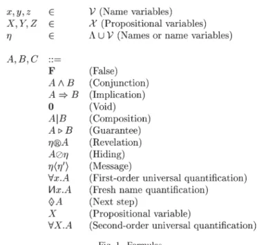
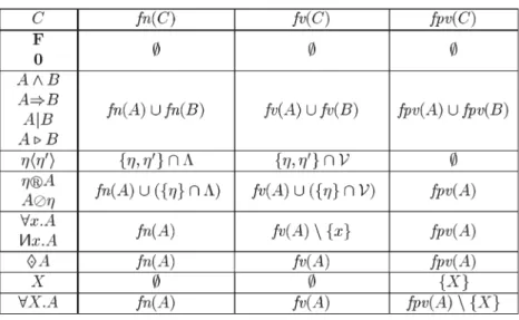
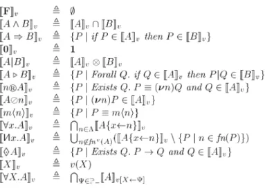
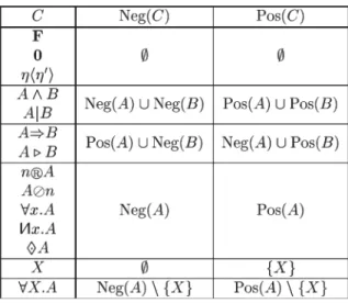
A spatial logic for concurrency (part I)

Ousasse apontar algumas hipóteses para a solução desse problema público a partir do exposto dos autores usados como base para fundamentação teórica, da análise dos dados

Para tanto, é necessário que a gestão Democrática seja vivenciada no dia a dia da escola (Projeto de Gestão da Unidade Escolar Gênesis; grifos meus). Essa parte do Projeto de

Table 6 Phenotypic virulence characteristics and PCR results for the presence of inv, ail, yst and virF virulence genes in the 144 Yersinia strains isolated from water and

Pré-avaliação sobre a compreensão dos princípios fundamentais: para soluções e colóides, equilíbrio de fase, electroquímica e química

2R L ) is computed using the expected load resistance value and not the actual ones, rending thus, respectively, smaller and higher values than expected. The measurements provided

This log must identify the roles of any sub-investigator and the person(s) who will be delegated other study- related tasks; such as CRF/EDC entry. Any changes to

Além disso, o Facebook também disponibiliza várias ferramentas exclusivas como a criação de eventos, de publici- dade, fornece aos seus utilizadores milhares de jogos que podem

- 19 de maio: realizou-se em Brasília audiência com o Secretário Geral do Ministério das Relações Exteriores do Brasil, Ministro Antonio de Aguiar Patriota, acompanhados do