Measuring corruption: what have we learned?

(1)

MEASURING CORRUPTION: WHAT HAVE WE LEARNED?

George Avelino†, Ciro Biderman‡ and Marcos Felipe Mendes Lopes§

ABSTRACT: There is current a large concern with corruption around the world as it may

be one of the causes for lagging development. There is also a concern that corrupt government will succeed to stay in power using the money obtained in corruption activities to finance political campaigns. Consequently, corruption might jeopardize economic development for a long period of time and questions democracy. To test the consequences and causes of corruption we need to measure the phenomenon. Traditional measures rely on perception surveys despite the shortcomings of these measures. Field and natural experiments or even survey experiments are other alternatives to measure the phenomenon. In this paper we review the measures available in the literature and propose an index based on objective information from random audit reports. We show that this index is a tool to analyze municipalities in Brazil and that our index is consistent with expected (stylized) behavior, it is relatively easy to compute, and it is normalized between 0 and 1.

KEYWORDS: corruption, measurement, corruption data, governance, local government. JEL Classification: H50, H75, H83.

(2)

MEDINDO CORRUPÇÃO: O QUE NÓS APRENDEMOS?

George Avelino†, Ciro Biderman‡ and Marcos Felipe Mendes Lopes§

RESUMO: Existe no mundo hoje em dia uma grande preocupação com corrupção. Há uma

percepção geral de que a corrupção pode ser uma das causas para o desenvolvimento tardio. Também há uma preocupação de que governos corruptos seriam bem sucedidos em manter-se no poder utilizando-se do dinheiro obtido com atividades corruptas para financiar suas campanhas eleitorais. Consequentemente, a corrupção pode comprometer o desenvolvimento econômico por um longo período de tempo e também colocar em xeque a democracia. Para testar as consequências e causas da corrupção é necessário, antes de tudo, medir o fenômeno. As medidas tradicionais partem de pesquisas de percepção com todos os problemas relacionados a essa medida. Experimentos naturais e de campo, ou até experimentos com pesquisa de campo são outras alternativas para medir o fenômeno. Neste artigo revisamos as medidas disponíveis na literatura e propomos um índice baseado em informações objetivas de relatórios de auditoria aleatória. Mostramos que o índice proposto é uma ferramenta para analisar municípios no Brasil, consistente com o comportamento (estilizado) esperado, relativamente fácil de computar e normalizado entre 0 e 1.

PALAVRAS-CHAVE: corrupção, medidas, dados sobre corrupção, governança, governo

local.

Classificação JEL: H50, H75, H83.

(3)

1. INTRODUCTION

The term corruption derives etymologically from the latin corruptio, which means deterioration. The World Bank definition states that “corruption is the abuse of public office for private gain”. This is similar to Portuguese dictionaries' definition, focusing on public servants’ behavior.

Given its relevance and impact on economic activity as a whole, the theme is recurrent in the economics literature. Crime in general is a major theme in economics at least since the seminal paper by Becker (1968). In Becker's “crime and punishment” model, there is an optimal amount of enforcement and "size" of the penalty that minimizes social lost. In 1975, Susan Rose-Ackerman develops what can be considered the first research paper dealing specifically with corruption, analyzing the relationship between market structure and the incidence of corruption in government contracting process. Since then, several studies, both theoretical and empirical, have used different models to describe the behavior of agents engaged in corruption-related practices.

Studies on the phenomenon of corruption evolved significantly over the past four decades, but no consensus has been reached on how to deal with the problem. Due to the different approaches used by researchers, the diverse theoretical conclusions about the causes and consequences of the phenomenon are currently under debate and imply in distinct empirical approaches.

A large part of the models use principal-agent theory to understand corruption. Usually the state is the agent (represented by an elected official and the bureaucracy) while the citizen-voter is the principal (BECKER, STIGLER, 1974; ACKERMAN, 1975; BANFIELD, 1975; ROSE-ACKERMAN, 1978). Based on principal-agent models, several scholarships investigated the impacts of corruption on the allocation of public resources, reaching diverse conclusions. Firstly, the existence of many governmental agencies (or, alternatively, public servants) offering the same service may reduce corruption, due to the competition for the rent to be extracted from the government (ROSE-ACKERMAN, 1978).

Antagonistically, with a weak central government, the existence of “multiple non-coordinated bureaucracies” may generate excessive rent extraction, reducing investments and, consequently, economic growth. Additionally, due to its illegal nature and demand for secrecy, corrupt activities distort resource allocation even further, towards investments in which cost

(4)

assessment and corruption detection are more complicated. Those procedures are usually not the most efficient choices (SHLEIFER, VISHNY, 1993; MAURO, 1998).

Other models emphasize the interaction between public and private agents to define an illegal payment in exchange for a public good or service. As a result, for example, Cadot (1987) highlights the relationship between public servants’ wages and decision-making powers, and Macrae (1983) emphasizes the relationship between the number of private agents demanding benefits and the occurrence of corruption.

In this article central government (the Union) is the principal (as the one that transfers resources to sub-national governments) and local governments are the agents (recipients of federal transfers and responsible for the provision of certain public services). Therefore, and considering the existence of asymmetric information favoring local governments, the main goal is to understand the role of federal oversight authorities as monitoring mechanisms capable of limiting the opportunistic behavior of local officials, when it comes to the allocation of federal grants.

2. THE MEASUREMENT PROBLEM

In parallel to the theoretical advances in modeling corruption, measuring it has also been advancing. Even though investment risk analysis organizations have developed methodologies to “measure” corruption1, no academic research has dealt with the issue until early 1990s. In 1995, Transparency International, an anti-corruption non-governmental organization, developed a methodology for calculating an index to measure perceived corruption – the Corruption Perceptions Index (CPI)2. Since 1996, the World Bank calculates the Worldwide Governance Indicators, comprising an indicator of the level of corruption called the “Control of Corruption Index”.

Based on these data, empirical research has investigated correlations between corruption occurrence and countries’ structural and institutional characteristics. Another branch of the literature investigated the effects of corruption-related practices on economic growth. Mauro (1995) using a cross-country analysis, concludes that corruption reduces investments and, thus, economic growth. Corruption is also claimed to be responsible for reducing the productivity of public

1_{The most important is the International Country Risk Guide, which comprises a measure of corruption, and is} calculated by Political Risk Services Group since 1980. The Index of Institutional Quality - Corruption¸ is calculated by The Economist Intelligence Unit.

2_{The number of countries for which the index is calculated increases significantly over time, from 41 in 1995 to 178 in} 2010.

(5)

investments (TANZI, DAVOODI, 1997) and the level of foreign direct investments (WEI, 2000), for distorting the composition of government expenditures (SHLEIFER, VISHNY, 1993; MAURO, 1998), and for increasing the degree of informality in the economy (JOHNSON, KAUFMANN , ZOIDO-LOBATÓN, 1998).

2.1. PERCEPTION-BASED INDICATORS: PROS AND CONS

Despite notably based on subjective data, corruption perception indexes have some advantages. First of all assembling data from different sources, it increases the sample size, making large cross-country analysis possible (SPECK, 2000). Second, aggregating several individual indicators, it reduces measurement errors and individual indicators biases (KAUFMANN, KRAAY, MASTRUZZI, 2006). There are, however, relevant drawbacks on using exclusively these indicators to identify causal relationships involving corruption. In spite of high correlations between perception indexes and objective data on corruption, the perception built-in biases may lead to the proposition of inadequate public policies (OLKEN, 2009). Among the characteristics that bias perceptions, Olken highlights the ethnic heterogeneity, the level of social participation and of transparency, and the educational attainment of respondents.

Consequently, subjective indicators should be used with caution in empirical research, and “[...] there is little alternative to continuing to collect more objective measures of corruption, difficult though that may be [...]” (OLKEN, 2009, p. 963), so that empirical findings become more precise and relevant. Complementing the argument, and reinforcing the necessity of obtaining “less subjective” indicators, Treisman (2007) argues that “[...] subjective data may reflect opinion rather than experience, and future research could usefully focus on experience-based indicators” (TREISMAN, 2007, p. 211).

Additionally, another risk of using perception-based indicators refers to the relationship between macro and microenvironments. According to Svensson (2005), research on corruption should determine the relationship between the macro and micro dimensions, not only establishing how institutional arrangements affect corruption, but also investigating how the occurrence of corruption may vary within the same institutional context. In other words, adding individual opinion on corruption may not make it through an aggregate (consistent) index. For instance, a country performing well will probably induce a better (general) perception of this country by businessmen regardless of the corruption level.

(6)

2.2. Objective measures: surveys, field experiments and internal control reports

Recently some research projects have been working with objective measures that could be associated with corruption, directly or indirectly. The usual source of information is derived from specific surveys or internal control audits. Evidently each approach has advantages and disadvantages in terms of efficiency, applicability and cost.

Di Tella e Schargrodsky (2003) used the prices paid for basic hospital inputs during an anti-corruption campaign in Buenos Aires, Argentina. They conclude that prices are, on average, 15% lower during the crackdown. Although limited in scope and coverage (Buenos Aires public hospitals), the main advantage of using data generated by an anticorruption program, is that there are no additional costs in generating the database. The main disadvantage, in this case, is that the anti-corruption program is not part of a permanent public policy. It was implemented just due to a scandal in the Argentinean health system.

Using a Public Expenditure Tracking Surveys (PETS), Reinikka and Svensson (2004) evaluated data on intergovernmental transfers for educational programs in Uganda. The conclusion is that, on average, schools received only 13% of the transfers they were entitled to, and most of them did not receive any resource at all. Using also a tracking survey, Olken (2006) concluded that 18% of the resources of a redistributive program in Indonesia had been “consumed” by corruption, between central government disbursement and local service delivery.

These two studies are similar in the way of measuring corruption. Both of them use surveys to track the resource flow, gauging “[...] the extent to which public resources actually filtered down to facilities” (REINNIKA, SVENSSON, 2004, p. 684). The advantage is that costs are not significantly high, but higher than those incurred by Di Tella and Schargrodsky (2003). Again, it is noteworthy the limitation in scope and coverage, since only part of the expenditure is “tracked”: education grants in Uganda and social welfare expenditure in Indonesia.

Another alternative found in the literature is to rely on field experiments. Olken and Barron (2009) using a field experiment specifically designed to directly observe the payment of bribes, point out that “[...] corrupt officials use complex pricing schemes, including third-degree price discrimination and […] two-part tariffs” (OLKEN and BARRON, 2009, p. 417). The findings indicate that, on average, 13% of the total costs of truck trips were constituted by illegal payments.

(7)

Theoretically, this research design is the most accurate when it comes to corruption measurement, since it is designed specifically for this purpose. However, costs incurred are significantly high, it is difficult to replicate and, despite its robust internal validity, external validity is questionable.

In line with the work proposed herein, Ferraz and Finan (2008, 2011) and Ferraz, Finan and Moreira (2009) use data from a random audits program established by the Office of the Comptroller General in Brazil. Ferraz and Finan (2008) evaluate the impact of the release of audit findings on the electoral performance of incumbents, concluding that the public dissemination of corruption in local governments had a significant impact on the likelihood of reelection (reducing it by 7 percentage points). Ferraz and Finan (2011) investigate whether political and electoral institutions affect corruption levels, finding that mayors that can be reelected are associated with significantly less corruption. Finally, Ferraz, Finan and Moreira (2009) find, additionally, evidence of links between corruption prevalence and educational attainment, reducing, in the long run, the accumulation of human capital and, therefore, economic growth.

Based on the fact that this measurement uses the “byproduct” of a governmental monitoring initiative, this indicator is 1. comprehensive in the sense that it covers the main expenditures of any municipality (education, health and social welfare)3; 2. the program is, in theory, permanent and; 3. municipalities are chosen randomly increasing the reliability of the data. Since data is available for all citizens, the main cost of constructing this index is classifying the audit reports. By instituting this program, the Brazilian Federal Government provided meaningful subsidies for the creation of objective indexes of corruption. Moreover, the policy itself is a relative inexpensive way to monitor local governments that may be easily replicable from the technical point of view.

Assuming that governmental agencies of internal and external control (notably the offices of the comptroller general and supreme audit courts) of several countries have auditing programs, the possibility of using the information generated by these programs certainly deserves a serious evaluation. One may consider that the monitoring activity is an end in itself, and that its byproducts, that may be used in order to evaluate the occurrence of corruption, can be considered an unintended positive gain of this public policy.

3_{Since most municipalities in Brazil have 80% or more of their revenues from Federal Grants, we believe that at least} half of total expenditure is (potentially) audited in the sample analyzed by the CGU (municipalities with less than 500 thousand inhabitants).

(8)

It is worth mentioning, however, that we do not intend to propose a definitive measure of corruption: the idea is to lie upon readily available data and formalize a methodology to quantify the occurrence of corruption objectively, which may be replicated by other governments.

3. THE BRAZILIAN RANDOM AUDITS PROGRAM

After the 1988 Brazilian Constitution, federal grants to state and local governments increased considerably and these federative entities assumed new responsibilities in public service delivery. However, no enforcement mechanisms to guarantee that these resources would be properly managed were introduced, putting into risk this new institutional arrangement.

One of the initiatives to respond to this risk was the Random Audits Monitoring Program created in 2003. The objective was to process special investigations of federal grants to State and local governments, through the Office of the Comptroller General (CGU).

According to the Contract Theory (HART, MOORE, 1988), if the definition of intergovernmental grants took place without the concurrent creation of enforcement mechanisms capable of limiting mayors’ opportunistic behavior, principal-agent conflicts could have arisen, leading to the need for renegotiation. In order to restrict unanticipated non-aligned behaviors, it is rational for the principal to introduce mechanisms to align his incentives with the agent’s.

In the case at hand, the random audits program constitutes a mechanism capable of limiting the opportunistic behavior of local public officials, when it comes to the allocation of federal grants that are typically earmarked.

Considering the fact that the random audits program is run by a governmental agency, there is the risk that the program will be captured by the bureaucracy and, therefore, ineffective as a tool for preventing corruption. However, the selection mechanism was designed to curb political influence – states and municipalities are selected in conjunction with the national lottery, witnessed by representatives of the press and members of political parties and the civil society. This randomness constitutes the gist of the random audits program, as it offers a unique research design opportunity and protects the program against some political arrangement such as logrolling.

(9)

So far, 34 lotteries have been draw, selecting more than 1800 local governments (municipalities). It is noteworthy, however, that the initially proposed periodicity has never been truly obeyed, due to political pressures - such fact seems to indicate that the program is an effective anti-corruption tool.

The random audits program investigates all federal grants to municipalities but focus on health, education and social welfare. Other areas such as communications, tourism, transport and others are investigated in some specific cases and usually those areas are randomly selected as well4.

The selection process has been designed in a way that samples are geographically representative. Currently, the probability of selection is around 1% for each of the 5526 municipalities (or 99.32% of Brazilian municipalities) under the threshold of 500,000 inhabitants, legally eligible to participate (representing approximately 70% of the Brazilian population).

We emphasize that the auditing process is guided by clear rules, and auditors are supposed to report findings based on clear evidence. There is the possibility of justification by the local public official, who may disagree with the determination of CGU’s technicians, and present evidence of appropriate behavior. In this case, the auditor may accept the arguments or not (and maintain the “non-compliance” evidence). These clear rules ensure that the findings associated with corrupt-practices are "as objective as they might be".

4. CORRUPTION AND MISMANEGEMENT INDICES BASED ON OBJECTIVE DATA

The algorithm to code the audit reports has been developed at the Center of Politics and Economics of the Public Sector - Getulio Vargas Foundation (CEPESP-FGV) since 2007, with financial support from the World Bank, from the United Nations Office on Drugs and Crime and from GV Pesquisa. The purpose was to assess the management of local government public policies.

After a municipality is selected to be audited, CGU compiles a database with all federal grants received by the local government on the current year and the two previous years. Some grants are randomly selected while others are necessarily audited. Based on the grants to be audited CGU headquarter prepare Service Orders (Ordens de Serviço – hereafter OS) detailing what should

4_{The CGU has focused more and more in health, education and social welfare. These 3 areas are typically responsible} for 2/3 of municipality expenditure and most municipalities own revenues are bellow 20% of total expenditure.

(10)

be audited in each grant. Then, a team of (regional) auditors visit the municipality and scrutinize everything connected to the selected grant, from the first disbursement to service delivery. As soon as the fieldwork is concluded, auditors prepare the report.

Using the published report research assistants (RAs) at CEPESP-FGV are randomly assigned to read and code each report. The auditor may make several "findings" for each OS. The RA codes each finding and each report is coded twice, by two different RAs. The codifications are then paired and checked by one of the research coordinators for consistency. With the support of UNODC we developed software to code and match the double entries.

In order to avoid the risk of wrongly classifying as corruption findings that are actually connected to mismanagement, we only consider as corruption-related practices the findings clearly linked with corruption. Of the 35 original categories (detailed in the Appendix) that include compliance, mismanagement and corruption, Table 1 shows the 7 categories of irregularities considered as corruption to calculate the proposed indicator detailed bellow.

-- Table 1: insert here --

In brief an OS may have no findings5_{(total compliance) or several findings by the auditor.} The findings may be connected to corruption or to mismanagement. Consequently an OS may have several findings related to corruption and several connected to mismanagement. It is also important to notice that we can relate corruption just to procurement6. This is consistent with corruption definition. We can identify corruption just when there is a monetary transaction. We will return to this issue later.

In this paper we propose and describe two (related) corruption indices. We work with the OS as our unit of observation. If there is at least one finding connected to corruption, the OS is considered as "corrupt". Our indices basically estimate the proportion of corrupt OSs on the total number of OSs issued by the CGU. More formally:

(1)

5_{Findings that are not connected to the municipality (e.g. it is related to the State Government) are also included in the} "no finding" category.

6_{We are not stating that there is corruption just in procurement but that the way corruption is defined you can identify} corruption just in procurement. This is true for any objective index we know.

(11)

(2)

Where com is the number of findings connected to corruption in municipality m, OS o; Om is the total number of OSs investigated in municipality m; 1(•) is the index function that, in this case, will be 1 if com>0; vom is the amount of the grant investigated by OS o in municipality m; Vm is the total amount of grants investigated in the municipality (i.e. ∑vom). In short, the numeric index of corruption (CNm) is the proportion of grants investigated that have at least one evidence of corruption; the monetary index (CVm) is the monetary proportion of grants connected with at least one corruption finding.

To construct such an index we have to ignore our "finest" scale: the finding. An OS would be classified as "corrupt" regardless of the number of findings connected to corruption. We are not very concerned with this problem however for a couple of reasons. First there is no rule on the number of findings reported by the auditors. One auditor may report the same problem in one item or in many. Second, we have no idea on the size of each item. Two findings representing 5% are the same as one finding representing 10% of the total amount. So, we do not believe that the number of findings may be a proxy for the intensity of the problem.

The second "missing opportunity" was discussed before: we can observe corruption only in procurement. So, the denominator of the indices proposed above will be inflated. A better index should measure the proportion of procurement processes investigated by the auditor that were connected to corruption. The difficulty in building such an index is finding out if the OS is connected to procurement or not. Our initial analysis on the description of the OS ("Objeto de Fiscalização") however suggests that it may be feasible to build an heuristic for defining if the item to be audit is connected to procurement or not. We are currently working on this refinement of the database.

Differentiating procurement from other types of investigations would allow us to build also an index of (public) mismanagement that is not inherently correlated with the corruption index. The index would use just OSs not related to procurement and redefine com as the number of findings

(12)

connected to mismanagement.7 Notice that we could include mismanagement in procurement as well since we have four categories in procurement that we did not considered as corruption.8 So it is possible to build an index of mismanagement considering all items. Consequently, the mismanagement index would be independent of the definition of the investigation (related to procurement or not). However this index would be naturally correlated to the corruption index if we cannot compute the corruption index using just procurement investigations.

The indices proposed are similar to Ferraz and Finan (2011) that define their (principal) indicator as "[...] the total amount of resources related to corrupt activities, expressed as a share of the total amount of resources audited" (p.1283). This would be equivalent to our monetary index. They also consider "the share of service items associated with corruption" that would be related to the numeric index9_{. Evidently their indices have the same shortcomings discussed above. We will} claim below that our indices are more precisely estimated. However, we believe that the main contribution of this paper is proposing an algorithm for estimating such an index and explicitly discussing the difficulties, possibilities and virtuosity of the indices. The original insight on these indices came from Ferraz and Finan (2011).

The first difference is that Ferraz and Finan (2011) did not have access to all service orders OS for each municipality. So, they have to work just with OSs reported by the auditor. This may cause bias, because many of the audited items for which there are no irregularities are excluded from the final report (especially before the 20th drawn). We have access to all OSs thanks to an agreement with CGU that kindly furnished a comprehensive list of all OS issued for this program. We do not believe that this imprecision would change Ferraz and Finan (2011) results. Actually it is possible that their results would be even more robust (by the golden rule). However, if we want to use the index to classify municipalities by the level of corruption we do need more precision to reduce classification errors (Type I and II).

Given the lack of information about the OS identification number, Ferraz and Finan (2011) cannot link their data with Union accounts. It means that their database cannot be used to analyze e.g. a federal program such as the "family health program" (Programa Saúde da família).

7_{In general, in this case, c}

om will be the number of items pointed out by the auditor except that some (rare) findings may not be considered since they are connected with some other institution instead of the municipality itself.

8_{Licitação: Ausência de divulgação; Licitação: Erros na documentação; Licitacao: modalidade inadequada ou} parcelamento de valor para evitar processo licitatorio and Licitacao: nao realizacao de licitacao

9_{They also consider " the number of irregularities related to corruption". However, we do not believe that this is an} index since municipalities with more OSs would naturally have more (observed) irregularities. We are not questioning the validity of their (alternative) dependent variable that, in the article, was used as a robustness test but it does not make sense for our purposes in this article.

(13)

Furthermore, as discussed above, just part of Union grants was actually audited. We have no idea how could they assert that "[...] corruption in local governments is responsible for losses of approximately US$550 million per year" (FERRAZ e FINAN, 2011, p. 1275). The auditor rarely reports the amount actually stolen. Since there is no hint on how they find such amount, we believe that they estimate it using the share of total federal resources transferred to municipalities that is associated with fraud and multiply it by total municipal grants from the Union. So, they implicitly assume that, if there is a fraud, 100% of the amount would be stolen. This is a quite strong assumption. Also since they do not match their data with Federal accounts they are not considering that not every grant is actually audited.

In the research supporting this article we documented all criteria to classify each auditor finding. This documentation (in Portuguese) is available upon request. Furthermore we link each classified finding with the OS identification number and consequently to the program and sub-program related to the item audited. Since we use 34 different classifications (see the Appendix) and kept the objective of the OS it would be possible to e.g. separate problems related to procurement from other type of problems (by definition related to mismanagement). Finally we develop web-based software to classify the reports making the process more reliable and easier to manage.

5. DATABASE

We were able to classify for this article the parts of the report related to the ministries of health and education10 around 330 municipalities. An assistant is able to classify around 10 municipalities for one ministry per week. We have been working with 4 to 5 undergraduate assistants. Since we have the double entry system discussed above, we were able to classify 80 to 100 municipalities (for one ministry) per month. Since we collect data for 8 months we would expect from 320 to 400 classifications to be completed11. We believe that being above the lower limit is quite good since we have to face turnover in the assistants, delays during student's exams, etc.

To be more precise, we attempt to classify 336 municipalities for audits related to the ministry of health. However, six municipalities did not have any OS related to this ministry. From those 336 municipalities we were able to classify 327 municipalities for audits related to the ministry of education. We build indices of corruption for the ministry of health, the ministry of

10_{Those two ministries are responsible for 40% or more of total grants from the Federal government.} 11_{(80 classifications X 8 months)/2 ministries = 320.}

(14)

education and combining those two ministries12 for 327 municipalities. Combining those two ministries is key in actually using the index. Notice that if there were just one OS in a municipality the index would be either 1 or 0. So, we are not very confident with the index for cases with very few observations13. In our sample, 209 municipalities have less than 6 OSs in the ministry of health and 201 in the ministry of education. However, just 15 municipalities have less than 6 OSs for the 327 municipalities for which we have coded both the ministry of health as the ministry of education.

The mean index is not very different if we consider the two ministries pooled or if we consider each ministry separately. In any case we have enough variance. The numeric index seems to be more biased towards lower values than the monetary index14_{. Notice that the 75 percentile is} always larger for the monetary index than for the numeric counterpart. It is also true that the mean is always larger for the monetary index although, with such a large variance, we cannot reject the hypothesis that the means are identical for any reasonable level of significance.

When we look at the whole distribution we can notice that the monetary index is smoother than the numeric index and that combining heath and education is smother than looking at just one ministry. The latter is expected since, as discussed, the index for only one ministry may have too little observations for the law of large numbers to work. It was not expected "ex-ante" that the monetary index would be smoother. We may hypothesize that weighting for the value of the transfer would be more precise in the sense that would better calibrate the index. However, we cannot ignore that the monetary index will eliminate OSs without an amount connected to it so the sample problem will be more dramatic for this index.

12_{Given this distinction we should review equations (1) and (2) to include another subscript referring to the ministry} under analysis and do the summation just for the appropriate ministry. We believe that this formalism would not add for the conceptualization of the index while adding in (unnecessary) syntax complexity.

13_{In other words, the index for one municipality is also a random variable since the audited items were randomly} selected. Consequently the index for the universe of grants received by the municipality is estimated from this sample of specific grants.

14_{We missed some extra observations in the monetary index since some OSs do not have a monetary value connected} to it. If all OSs in a given municipality did not have a monetary value, we cannot compute de monetary index for this municipality.

(15)

-- Graph 1: insert here -- -- Graph 3: insert here --

Despite the differences in precision, each index probability distribution function (p.d.f.) is similar. The distribution is increasing for very low indices (below 0.05) and then decreasing monotonically. This is not exactly observed for the p.d.f. for the monetary index for education. In this case the distribution falls very fast until 0.3 and then is it flattens. Also for the monetary index pooling health and education we can notice a change around 0.2 when the distribution flattens.

So, we cannot see considerable differences between the distribution of the indices for one ministry or the other or combining both. The main differences are between the numeric and the monetary indices but even those are not considerable. It means that indices for a particular ministry might be feasible to be constructed although we would not recommend constructing a municipal index by ministry. We do not have precision for that. However, it suggests that it would be possible to use the index by ministry as a dependent variable.

If the indices were totally related it would indicate that a corrupt municipality would be corrupt in any sector. It would make it not so interesting to decompose the index in this way since it would be possible to use one or the other. In other words, one index would not add relevant information to the analysis. On the other hand, if the indices were not related at all it would not be reasonable to make an index pooling all sectors at the same time.

Table 3 correlates all indices and brings some good news. The numeric and the monetary indices are highly correlated suggesting that we can use either in an analysis that the results are not likely to change. On the other hand, indices for health and education are highly correlated with the indices pooling those two ministries suggesting that it is may not be problematic pooling them together to analyze the municipality as a whole. On the other hand the indices for different ministries are weakly correlated suggesting there is something to learn from the analysis of disaggregated indices.

(16)

6. CORRELATION WITH SOCIAL VARIABLES

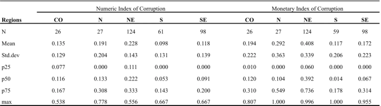
Although this article did not intend to make any analysis with the indices proposed, it is interesting to take the opportunity and check some expected correlations to understand if the indices are consistent with other findings in the literature. We were first interested with the regional characteristic of the indices. Looking at the corruption indices calculated for the five Brazilian macroregions, we can see that the North and Northeast regions of the country, notably the poorest, have the highest levels of corruption, both numerically and monetarily. The results are shown in Table 4.

By analyzing the regional prevalence of corruption, it is plausible to assume that there is a correlation between poverty levels and corruption prevalence, although it is impossible in such a analysis to clearly determine the direction of causality. Focusing attention on calculated averages, the Northeast region (with the lowest average per capita income) stands out with the highest corruption indicators, in both numerical and monetary terms. On the other side, the Southern region (with the highest average per capita income) shows consistently the lowest indicators of corruption.

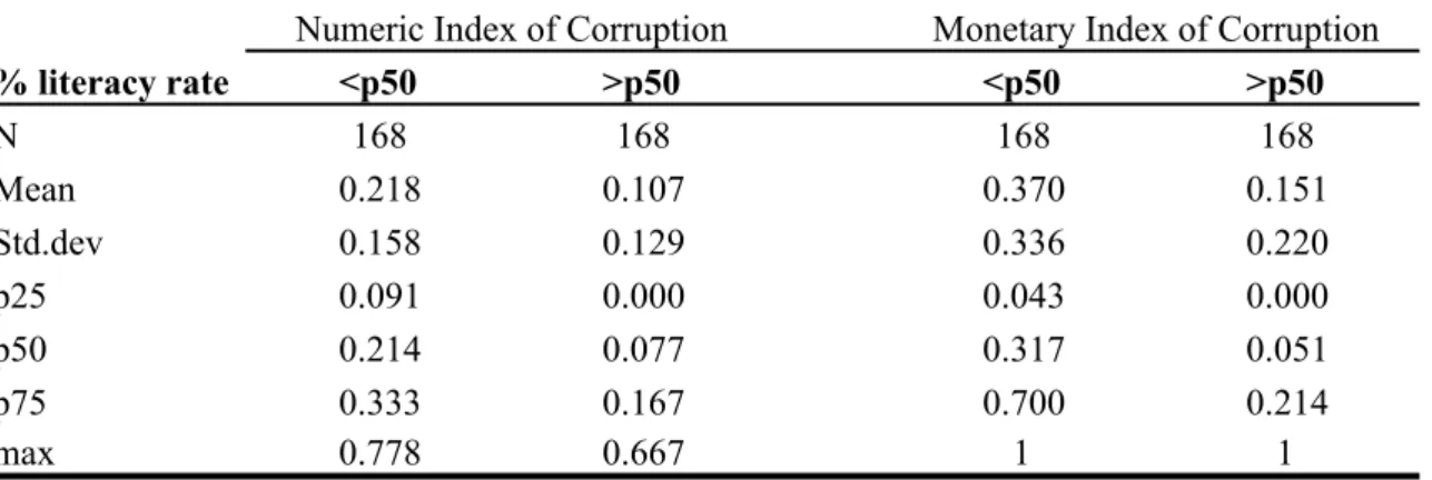
We repeat the same exercise separating municipalities above and bellow the median percentage of illiterates. This is connected to the idea that local average literacy rates are related with the observed levels of corruption in local governments. The results are shown in Table 5.

The difference between the two groups is evident: the group “p<50” comprises the municipalities with literacy rate below the sample median, and the corruption indicators are significantly higher than the group with municipalities with literacy rate above the sample median. These preliminary results are extremely startling, because they indicate that corruption directly affects lower income population. Once again the direction of causality is not being called into question: based on the assumption that corruption changes the allocation of resources, the poor may be more severely affected, since they depend heavily on the government for the provision of basic needs, such as health and education.

(17)

Finally we attempt to combine all social variables at once in a regression framework. In this framework we can search for correlations between municipal structural and political characteristics and corruption prevalence. The model comprises municipal structural characteristics; political characteristics; and state fixed effects. The covariates tested here are the same used in Ferraz and Finan (2008, 2011) and Ferraz, Finan e Moreira (2009).

Panels A and B in Figure 6 reveal that the sample under study is heterogeneous, encompassing municipalities with significant differences in demographic, economic, structural and political terms. This heterogeneity reflects the diversity of Brazilian municipalities, confirming the randomness of the selection process carried out by the Office of the Comptroller General through the national lottery system.

Evaluating the results presented in Table 8, we conclude that the proposed indices correlate to relevant variables in line with previous findings in the literature. On the other hand there are almost no robust correlation in the sense that most coefficients were not statistically significant. In any case, even if the estimated coefficients are not precise, the effects of the covariates on corruption are aligned with results previously achieved. In a nutshell, we may say that: the higher (or the better) the educational attainment of the population (GLAESER, SAKS, 2006), the infrastructure of municipal services (TRANPARÊNCIA INTERNACIONAL, 2008), and the access to information (REINIKKA, SVENSSON, 2005; FERRAZ, FINAN, 2008), the lower the observed levels of corruption; and conversely, the higher the income inequality, the higher the observed levels of corruption (USLANER, 2006).

7. CONCLUDING REMARKS

The use of corruption perception indicators was widespread over the past two decades but, recently, researchers have sought new ways to measure corruption based on actual objective findings. In Brazil, with the random audits program created by the Office of the Comptroller General, researchers have a rare opportunity to use a national public policy as the basis for building such an objective indicator.

(18)

Given the findings of Shleifer and Vishny (1993) and Mauro (1995) that corruption distorts the allocation of resources from investments in health and education towards those where the detection of corruption is more complex, a vicious circle is created. Poorer municipalities with lower literacy rates are those with the highest rates of corruption in Brazil. Higher corruption rates tend to further distort the allocation of public resources, affecting more severely the poorest population, which depends primarily on public provided services, increasing socio-economic inequality (GUPTA, DAVOODI, ALONSO-TERME, 2002; GLAESER, SAKS, 2004). With lower educational attainment, the local population is not able to exercise social control over the local public officials, generating further incentives for corruption to increase.

Although the indices proposed in this article are not new in the literature, we believe that we contribute to the literature discussing them more thoroughly and showing their shortcomings and advantages over other indices. The indices proposed in this article are potentially very promising for e.g. creating an index to rank municipalities in terms of corruption. The way we construct the database allow us to go further on the indices revealing more dimensions of this phenomenon that may be one of the reasons why some municipalities are still lacking behind.

8. REFERENCES

BANFIELD, E. C. Corruption as a feature of governmental organization. Journal of Law

and Economics, v. 18 n. 3, 29, p. 587-605, 1975.

BECKER, G. Crime and Punishment. Journal of Political Economy, v. 76, n. 2, p. 169-217, 1968.

BECKER, G.; STIGLER, G. Law Enforcement, Malfeasance, and Compensation of Enforcers. The Journal of Legal Studies, v. 3, n. 1, p. 1-18, 1974.

CADOT, O. Corruption as a gamble. Journal of Public Economics, v. 33, n. 2, p. 223-244, 1987.

DI TELLA, R.; SCHARGRODSKY, E. The Role of Wages and Auditing during a Crackdown on Corruption in the City of Buenos Aires. Journal of Law and Economics, v. 46, p. 269-292, 2003.

FERRAZ, C.; FINAN, F. Exposing Corrupt Politicians: The Effects of Brazil’s Publicly Released Audits on Electoral Outcomes. Quarterly Journal of Economics, v. 123, n. 2, p. 703-745, 2009.

______. Electoral Accountability and Corruption: Evidence from the Audits of Local Governments. American Economic Review, v. 101 n. 4, p. 1274-1311, 2011.

FERRAZ, C.; FINAN, F.; MOREIRA, D. Corrupting learning: evidence from missing federal education funds in Brazil. Working Paper, 2011. Mimeografado.

(19)

GLAESER, E.; SAKS, R. Corruption in America. Journal of Public Economics, v. 90, n. 6-7, p. 1053-1072, 2006.

GUPTA, S.; DAVOODI, H.; ALONSO-TERME, R. Does corruption affect income inequality and poverty? Economics of Governance, v. 3, p. 23-45, 2002.

HART, O.; MOORE, J. Incomplete contracts and renegotiation. Econometrica, v. 56, n. 4, p. 755-785, 1988.

JOHNSON, S.; KAUFMANN, D.; ZOIDO-LOBATÓN, P. Regulatory Discretion and the Unofficial Economy. American Economic Review (Papers and Proceedings of the Hundred and Tenth Annual Meeting of the American Economic Association), v. 88, n. 2, p. 387-392, 1998.

KAUFFMANN, D.; KRAAY, A.; MASTRUZZI, M. Measuring corruption: myths and realities. World Bank, Working Paper, 2006.

MACRAE, J. Underdevelopment and the economics of corruption: a game theory approach.

World Development, v. 10, n. 8, p. 677-687, 1982.

MAURO, P. Corruption and Growth. Quarterly Journal of Economics, v. 110, n. 3, p. 681-712, 1995.

______. Corruption: Causes, Consequences and Agenda for Future Research. Finance and

Development, março, 1998.

OLKEN, B. Corruption and the costs of redistribution: Micro evidence from Indonesia.

Journal of Public Economics, v. 90, n. 4-5, p. 853-870, 2006.

______. Corruption perceptions vs. corruption reality. Journal of Public Economics, v. 93, n. 7-8, p. 950-964, 2009.

OLKEN, B.; BARRON, P. The simple economics of extortion: evidence from trucking in Aceh. Journal of Political Economy, v. 117, n. 3, p. 417-452, 2009.

REINIKKA, R.; SVENSSON, J. Local Capture: Evidence From a Central Government Transfer Program in Uganda. The Quarterly Journal of Economics, v. 119, n. 2, p. 679-705, 2004.

______. Fighting corruption to improve schooling: evidence from a newspaper campaign in Uganda. Journal of the European Economic Association, v. 3, n. 2-3, p. 259-267, 2005.

ROSE-ACKERMAN, S. The economics of corruption. Journal of Public Economics, v. 4, n. 2 p. 187-203, 1975.

______. Corruption: A study in political economy. New York: Academic Press, 1978. SHLEIFER, A.; VISHNY, R. Corruption. Quarterly Journal of Economics, v. 108, n. 3, p. 599-617, 1993.

SPECK, B. Mensurando a corrupção: uma revisão de dados provenientes de pesquisas empíricas. In: Os custos da corrupção. São Paulo: Fundação Konrad Adenauer, 2000.

(20)

SVENSSON, J. Eight questions about corruption. Journal of Economic Perspectives, v. 19, n. 3, p. 19-42, 2005.

TANZI, V.; DAVOODI, H. Corruption, Public Investment and Growth. IMF Working

Paper 97/139, 1997.

TRANSPARENCY INTERNATIONAL. Global Corruption Report 2008 – Corruption in

the Water Sector, London, UK: Pluto Press, 2008.

TREISMAN, D. What have we learned about the causes of corruption from ten years of cross-national empirical research? Annual Review of Political Science, v. 10, p. 211-244, 2007.

USLANER, E. Corruption and inequality. United Nations Universtity – World Institute for

Development Economics Research, n. 34, 2006.

WEI, S. How taxing is corruption on international investors? The Review of Economics and

(21)

GRAPHS AND TABLES

Table 1: Auditors’ findings used for the computation of the corruption indicator

Private appropriation (no funds receipts);

Procurement infraction (ghost or non-existing companies); Procurement infraction (false documents);

Procurement infraction (tender favoring); Private appropriation (overpricing); Private appropriation (false receipts); Irregularities associated with corruption

Procurement infraction (false receipts, overinvoicing, etc.);

Source: CEPESP

Table 2: Descriptive statistics of the proposed corruption indicators

Index obs. mean std.dev p25 p50 p75 max

Numeric Index of Corruption 327 0.061 0.152 0.000 0.125 0.250 0.778

Monetary Index of Corruption 327 0.259 0.305 0.000 0.013 0.465 1.000

Numeric Index of Corruption - Health 329 0.183 0.215 0.000 0.143 0.250 1.000 Monetary Index of Corruption - Health 328 0.209 0.289 0.000 0.056 0.313 1.000 Numeric Index of Corruption - Education 327 0.158 0.207 0.000 0.000 0.273 1.000 Monetary Index of Corruption - Education 322 0.298 0.393 0.000 0.000 0.656 1.000 Source: CEPESP

Table 3: Correlation matrix for corruption indices

Numeric Index of Corruption Monetary Index of Corruption Numeric Index of Corruption - Health Monetary Index of Corruption - Health Numeric Index of Corruption - Education Monetary Index of Corruption - Education

Numeric Index of Corruption 1

Monetary Index of Corruption 0.7639 1

Numeric Index of Corruption - Health 0.8123 0.6201 1

Monetary Index of Corruption - Health 0.6695 0.7069 0.794 1

Numeric Index of Corruption - Education 0.7037 0.5576 0.2355 0.2365 1

Monetary Index of Corruption - Education 0.6204 0.721 0.2234 0.2127 0.8161 1

Source: CEPESP

Table 4: Corruption Index by Region in Brazil

Regions CO N NE S SE CO N NE S SE N 26 27 124 61 98 26 27 124 59 98 Mean 0.135 0.191 0.228 0.098 0.118 0.194 0.292 0.408 0.117 0.172 Std.dev 0.129 0.204 0.143 0.131 0.139 0.222 0.363 0.339 0.206 0.223 p25 0.077 0.000 0.111 0.000 0.000 0.010 0.000 0.060 0.000 0.000 p50 0.116 0.133 0.222 0.053 0.091 0.120 0.104 0.392 0.014 0.067 p75 0.167 0.308 0.333 0.143 0.200 0.310 0.549 0.736 0.178 0.314 max 0.538 0.778 0.556 0.667 0.667 0.807 1.000 0.996 1.000 0.955

Numeric Index of Corruption Monetary Index of Corruption

(22)

Table 5: Corruption indices by literacy rate % literacy rate <p50 >p50 <p50 >p50 N 168 168 168 168 Mean 0.218 0.107 0.370 0.151 Std.dev 0.158 0.129 0.336 0.220 p25 0.091 0.000 0.043 0.000 p50 0.214 0.077 0.317 0.051 p75 0.333 0.167 0.700 0.214 max 0.778 0.667 1 1

Numeric Index of Corruption Monetary Index of Corruption

Source: CEPESP

Table 6: Descriptive statistics of municipal and political characteristics

Variable N mean std.dev min max

Panel A: Municipal characteristics 336

Demographic density (hab/km2) 336 55.135 138.444 0.615 1777.166

Income inequality (índice de Theil) 336 0.522 0.107 0.310 1

Percentage of literates 336 76.957 12.785 39.339 95.706

Urbanization rate 336 57.187 22.480 4.668 100

Log (income per capita) 336 4.915 0.575 0.542 6.033

Percentual de domicílios com água encanada 336 65.831 30.350 0.340 99.734

Existence of local radio station (1/0) 336 0.494 0.501 0 1

Panel B: Mayors' characteristics 336

Age 336 47.7350 9.2890 22 78

Gender (1/0 - masculino) 336 0.9200 0.2720 0 1

Years of education 336 13.0710 3.3600 4 16

Observation: this table reports the descriptive statistics of variables to be used in the econometric model. Variable Log (income per capita) was obtained by calculating the neperian logarithm of income in 2000 current prices. Source: CEPESP

(23)

Table 7: Regression of corruption indices on municipal and political characteristics

(1) (2) (3) (4)

Income inequality (índice de Theil) 0.057 0.085 0.222 0.312

[0.073] [0.072] [0.165] [0.161]+

Percentage of literates -0.001 -0.001 -0.003 -0.004

[0.002] [0.002] [0.003] [0.003]

Percentage of house with water treatment -0.001 -0.001 -0.002 -0.002

[0.001]* [0.001]+ [0.001]+ [0.001]

Existence of local radio station (1/0) -0.01 -0.011 0.008 0.005

[0.018] [0.017] [0.033] [0.034]

Mayors' age 0 0 -0.001 0

[0.001] [0.001] [0.001] [0.002]

Mayors' gende (1/0 - male) -0.041 -0.026 -0.058 -0.033

[0.031] [0.031] [0.064] [0.064]

Years of education 0 0.001 0.001 0.003

[0.002] [0.002] [0.005] [0.005]

State intercepts? Sim Sim Sim Sim

Lottery intercepts? Não Sim Não Sim

Observations 336 336 334 334

R-square 0.31 0.4 0.33 0.38

Numeric Index of Corruption Monetary Index of Corruption

(24)

Graph 1: Probability Density Function for the

Numeric Index of Corruption (Health and Education) for Selected Municipalities

Graph 2: Probability Density Function for

the Monetary Index of Corruption (Health and Education) for Selected Municipalities

Fonte: CEPESP

Numeric Index of Corruption (Health) for Selected Municipalities

Monetary Index of Corruption (Health) for Selected Municipalities

(25)

the Numeric Index of Corruption (Education) for Selected Municipalities

the Monetary Index of Corruption (Education) for Selected Municipalities

(26)