A Microscopic-View Infection Model
based on Linear Systems
He Haoa, Daniel Silvestrea,b, Carlos Silvestrea,b
aDepartment of Electrical and Computer Department, Faculty of Science and
Technology, University of Macau, China.
bInstitute for Systems and Robotics, Instituto Superior T´ecnico, Universidade de
Lisboa, Lisboa, Portugal.
Abstract
Understanding the behavior of an infection network is typically addressed from either a microscopic or a macroscopic point-of-view. The trade-off is between following the individual states at some added complexity cost or looking at the ratio of infected nodes. In this paper, we focus on developing an alternative approach based on dynamical linear systems that combines the fine information of the microscopic view without the associated added complexity. Attention is shifted towards the problems of source localization and network topology discovery in the context of infection networks where a subset of the nodes is elected as observers. Finally, the possibility to control such networks is also investigated. Simulations illustrate the conclusions of the paper with particular interest on the relationship of the aforementioned problems with the topology of the network and the selected observer/controller nodes.
Keywords: Infection Networks; Source localization; Topology Identification; Linear Models; Controllability; Observability.
1. Introduction
The network topology identification problem refers to the challenge of de-termining the links or connections among the various components in a network. Current research trends relating to this topic include source localization and structure discovery that can be found in many applications in fields such as
Biology [1], Social Sciences [2], Computer and Electrical Engineering, Business, amongst others. In [3], network observability and source localization are dis-cussed for an infection network model. The time before all nodes are infected depends on the topology, namely on the nodes degree, i.e., the number of im-mediate neighbors.
Motivation for this work comes from the study of infection networks of peo-ple, namely for understanding outbreaks of diseases and infections in the world. In computer sciences, it may be useful to understand the spread of computer virus, exchange of P2P files or discover the topology of a network from the local measurements of distributed algorithms. We also envisage the case where one entity wants to estimate the network and is allowed to run a normal algorithm that exchanges local values with neighbors.
There is a vast body of work in the context of epidemics networks avail-able in the literature (the interested reader is directed to a survey of traditional techniques in [4]). Typically, the initial approach is to consider a mean field approximation of the infection process and then analyze what happens to the average case or the percentage of infected nodes in the network. One of the ear-liest works presented can be found in [5, 6] and additional study of the threshold dividing the cases of full infection or recovery is given in [7]. Such models pre-senting the evolution of the percentage of infected nodes have attracted a lot of attention both in continuous-time [8] and discrete-time [9].
Different variants of epidemics can be found in the aforementioned literature: Infected (SI), Infected-Susceptible (SIS), Susceptible-Infected-Recovered (SIR), and, additionally the Susceptible-Exposed-Infected (SEI) [10]. Other studies such as considering nodes entering and leaving in a stochastic fashion [11] and studying the evolution by explicit series solution of the SIR and SIS epidemic models [12] have also been considered. Nevertheless, all these approaches have shortcomings in the sense that only the macroscopic view is considered. If one would like to distinguish what happens to some indi-vidual nodes, other alternatives are required.
the epidemics as a group of nodes interconnected by a network that has a state indicating their current status: infected, recovered, etc. This normally entails the use of Markov Chains to model the infection process and examples can be found in [13, 14, 15, 16, 17]. These references investigate slightly different models either with self-infection links or not in order to discuss what is the threshold that leads the network to go to a full infected or disease-free state and how the topology contributes to the transient. The Markov approach is intrinsically a microscopic view that considers the individual states. Individual states will amount to exponential state space, i.e., if there are 2 possible states and n nodes it will be 2n, 3n if it is infected, susceptible and recovered, and so on. A clear trade-off occurs between the two approaches in the sense that the macroscopic loses important individual information but its description is amenable whereas the microscopic view focuses on the particular nodes but has an exponential state-space on the number of nodes. Efforts to analyze the Markov model and simplify the computation needed to check the steady-state of this large state space model have also been investigated in [18]. In [16] it is first computed the probability that each node is infected by any neighbors before computing relationships between the parameters that render a full infection or a disease-free network. In this paper, the approach is focused on the microscopic view in the deterministic setting where infected nodes will spread to their neighbors.
In this paper, the approach is to follow the model introduced in [3] as a way to have a microscopic view while avoiding the exponential growth of the state space by introducing a nonlinear operation on the state. The main objec-tive is to leverage the model and make it suitable for more general discussions. Three topics are of interest, namely source localization of the infection node (discovering who was the initial infected node that caused the epidemic), net-work topology identification (finding based on the measured output what is likely to be the interconnection among the various nodes), and being able to control the steady state in an optimized fashion for the simpler model (see [19] for a discussion on the control of the complex macro version of the SIR model). All problems are of practical interest in a real-world application: determining
who was the initial infected person or equipment; gathering information about the interconnections in the network from the measurements of how the virus or disease is spreading; controlling the propagation through a recovery process.
The subject being studied in this paper closely relates to that of Compressed Sensing where some signal is intended to be reconstructed based on a partial observation of the network state. In [20], the framework of compressed sensing is used to retrieve the sparse network topology for a dynamical linear system. The Least Absolute Shrinkage and Selection Operator (LASSO) have also been used in [21, 22] with an `1 penalty to ensure a sparse solution (the `1 norm is the sum of the absolute value of the entries of the vector and serves as a surro-gate to minimize the number of non-zeros elements and get a sparse solution). The herein proposed algorithm also adopts a similar penalty adjusted for our respective problem.
In [23], authors propose the design of a Bayesian network to estimate the probabilities associated with each connection in the network. A similar opti-mization can be posed to construct the sparsest probability transitions of the network from the data of the evolution of the state.
Recently, network identification problem has received a lot of attention by different research communities. For example in smart grids, topology identi-fication has been performed using convex optimization or voltage correlation analysis in order to optimize the power system efficiency in [24] and [25], re-spectively. In [24], a maximum a posterior-based mechanism, embedding the prior information on the breaker status, is proposed to enhance the identifica-tion accuracy. In [25], the goal is to reconstruct the topology of a poridentifica-tion of the power distribution network, given a dataset of voltage measurements. For Bayesian Networks (BNs), the authors in [26] proposed a BN structure learning algorithm to determine large-scale BN structures from high-dimensional data. The main idea also has some parallel to the concept of finding which links must be present in the network based on their likelihood given the measurements.
In [27] and [28], it is considered the diffusion of a rumor or virus in a large-scale network with deterministic propagation. Different models have also been
used with the purpose of determining the source of the infections based solely on local measurements of some states of other nodes [3], [29], [30] and [31]. The method in [29] makes use of the Minimum Description Principle (MDP) to find in an initial phase the more likely nodes to be classified as sources using the submatrix-Laplacian method, and then determining the actual source by a designed MDP. The localization of multiple sources is settled in [30], which builds the graph Laplacian matrix in order to standardize each eigenvector com-ponent. Resorting to a threshold, the network nodes are clustered by the time they emitted. Therefore, multiple sources can be localized through the knowl-edge of which nodes reduce the most the largest eigenvalue of the adjacency matrix after its removal. The deterministic propagation has also been tested using real data. In [31], a crawl of Twitter is used as a data set to a rumor detection and single source identification through a greedy algorithm.
In another direction, finding the source of the spreading process can be thought as the isolation of a fault occurring at one of the observed nodes. The task can be performed in a distributed fashion resorting to filters that encode each of the faults (i.e., each of the nodes injecting a non-zero signal) such as the work in [32] and [33] for the collaborative version where nodes share their estimates along with the normal procedure of the model. The models based on fault identification typically have the disadvantage that one needs to consider multiple combinations if more than one source is possible. Another point to notice is that fault identification for this case will be equivalent to the possible solutions to the observability equation so, in a sense, we are checking which fault signals have the smallest norm.
Contributions This paper relates to the aforementioned approaches of con-sidering a deterministic propagation [3], [27] and [28] instead of a stochastic (typically using a Markov Chain) version. Deterministic propagation entails that nodes become infected/informed depending on their neighbors and not as a result of a random variable, as well as their state remaining unchanged unless an additional process of cure is started. The intuitive idea is to avoid a complex description of a microscopic view of the propagation but retaining the same
granularity. To this end, a linear model is considered for the system followed by a non-linear operation corresponding to the observation. In a sense, this can be thought of as the underneath state of the linear system corresponding to the count of the virus and the saturation used to declare an infection when the number of virus is sufficient to overcome the defense response.
In a social network context, this can be interpreted as the most likely opinion of a person given the input he/she has received from his/her immediate contacts. The idea is inspired in the work [3] followed by a generalization to an unknown initial infection time. The source localization and network identification can then be revisited through a cardinality minimization problem relaxed to be an l1 minimization [34]. Leveraging this new approach, we are able to use linear systems techniques to obtain results on how to control the infection. A previous conference paper [35] from the same authors has already introduced the problem of network topology identification for the model with unknown infection time. This paper extends those results to the possibility of recovery and also studies the control aspect of the network.
The contributions of this paper can be summarized as follows:
• A general diffusion model is presented that considers unknown initial infec-tion time and can incorporate addiinfec-tional infecinfec-tion and recovery processes; • The formulation of the topology identification as a linear program for the
general model;
• Definition of the controllability of the infection process and how to com-pute control laws based on standard linear time-invariant systems theory; • Formalization of the optimal control strategy for the infection network. The remainder of the paper is organized as follows. We provide a descrip-tion of the SI and SIR diffusion processes in Secdescrip-tion 2. The source localizadescrip-tion problem and the observability of the proposed models are investigated in Sec-tion 3. SecSec-tion 4 describes the convex soluSec-tion for the network topology discov-ery problem under the diffusion models while Section 5 details the analysis of
the controllability and reachability of the infection networks in addition to pro-viding ways to compute minimum energy controls that drive the system to the full recovery or to any desirable configuration. Simulation results are presented in Section 6. Concluding remarks and directions for future work are offered in Section 7.
2. Infection Models
In the current section two models are detailed: Susceptible Infected (SI) where the nodes are either infected or susceptible to be contaminated; and the Susceptible Infected Recovered (SIR) which allows for nodes to return to a state with no virus. In the sequel, details are provided on how to write the SI and SIR models as a linear time invariant system with a nonlinear operation on the output. The following general notation is going to be used throughout the paper.
Notation : We let 1n := [1 . . . 1]| and 0n := [0 . . . 0]| indicate n-dimension vector of ones and zeros. Dimensions are omitted when no confusion arises. The vector eidenotes the canonical vector whose components equal zero, except component i that equals one. The notation kvk1:=P
n
i=1|vi| for a vector v. 2.1. Susceptible Infected (SI) model
A network of n components is defined by the node set V := {1, 2, · · · , n} and the edge set E ⊆ V × V containing all pairs (i, j) such that there exists a connection from node i to node j. We define the adjacency matrix A ∈ Rn×n representing the network structure corresponding to the set E.
Matrix A can be defined as
Aji= 1, if (i, j) ∈ E 0, otherwise . (1)
Moreover, throughout the paper it is assumed an undirected topology which implies that A is symmetric, i.e., A = A|.
Following the concepts in [3], a rumor or infection cannot be reversed and, therefore, the nodes are either susceptible to the infection or already infected. In the literature this model has been known as the Susceptible-Infected (SI) model. As a consequence, a single infected node at the initial time will result in all nodes receiving the infection at some point in the future, provided the network is connected. The process is deterministic and following [3], if a node is infected at discrete time t, all its neighbors will be infected at t + 1.
The infection state is denoted as a binary vector x(t) ∈ {0, 1}n, where entries equal to one in x(0) identify the infection sources. Naturally, for a connected graph, there exists a horizon N = n − 1 (i.e., the largest diameter of a n-node network) such that x(N ) = 1n, corresponding to a full infection. The vector of measurements y(·) ∈ {0, 1}m corresponds to the state of each m sensed nodes. Since y(·) represents the measurements from the sensors, matrix C will have a row per sensor with an entry equal to one corresponding to which node is being sensed (for example, if node 2 is being measured we haveh0 1 0 · · · 0
i , i.e., be equal to e|2). It is convenient to define the nonlinear operation that will give the status of a node given its internal infection count. The following notation applied to a matrix M:
Mij = 1, if Mij > 0 0, otherwise. . (2)
Additionally, let us introduce the transition matrix that takes the initial state to x(t) as:
Φ(t, tinitial) = At−tinitial+ At−tinitial−1. (3) Given the aforementioned definitions, the next theorem shows that the Susceptible-Infected (SI) dynamics can be modeled through a dynamical system perspective by considering a Linear Time-Invariant (LTI) followed by a nonlinear saturation function to get the status of each node. This result can be found in [3] and is added herein for completeness.
is equivalent to the dynamical system modeled by the equations: x(t) = Φ(t, 0)x(0)
y(t) = Cx(t)
, (4)
where Φ(t, 0) = At+ At−1.
The network state equation in Theorem 1 assumes the initial infection time is known and set to be the origin of the time index t. One of the objective of this paper is to elaborate on a model that can encompass many variations of infection networks. Initial time of infection is typically not known and for that reason we introduce a General Diffusion Model which assumes an initial zero condition and is subject to an exogenous excitation corresponding to the infection. As a consequence, we can have the input vector u(·) serving as the injection of the infection onto the source node at some later point in time. Therefore, we can write a related model with a state vector z(t) ∈ {0, 1}n and infecting vector u(t) ∈ {0, 1}n, having non-zero entries to signal new infections at time t. Given that u(·) accounts for all infection processes, we have z(0) = 0n. We also remark that multiple infections can be initiated at different time instants using this model and, as discussed later in the paper, that the u(·) vector can also be used as a recovery for the infection started at some origin node, resulting in the SIR model. In the next theorem we show that the General Diffusion Susceptible-Infected (GDSI) model is a shifted version of the DSI model. The proof can be found in Appendix A.1.
Theorem 2 (General Diffusion Susceptible-Infected (GDSI)). The DSI model in Eq. (4) without knowledge of the initial infection is equivalent to the dynamical system defined by the following equations:
z(t) = Φ(t, 0)z(0) + t−1 X τ =0 Φ(t, τ + 1)u(τ ) y(t) = Cz(t) , (5)
which can be rewritten as: z(t) = t−1 X τ =0 Φ(t − τ − 1, 0)u(τ ) y(t) = Cz(t) . (6)
A clear advantage of the GDSI model is that it allows to envisage other possible scenarios to be studied other than the SI model. In particular, Eq. (5) encompasses the SIR model and allows the case of nodes being healed and multiple infections outbreaks. In such cases, the signal u can have different types of values to model when an infection appeared in the network and when a cured was applied to a specific node.
2.2. Susceptible Infected Recovered (SIR) model
The SIR model assumes that nodes can return to a state of no infection by some exogenous action. The study of unknown initial state in Theorem 2 enables the introduction of more complex behaviors such as multiple infections and recoveries using the u(·) signal in our linear time-invariant version of the infection model in Eq. (5) with z(0) = 0n. By purposely choosing the input u(·), it is possible to simulate different types of rules for how infections and recoveries interact. In the following result, we present the case where the last infection/recovery is the most powerful and eventually dominates over the entire network. In a sense, the intuition behind Eq. (5) can be understood as the state z(·) accounting for the number of bacteria/virus minus the number of antibiotics/antivirals, followed by a saturation. Thus, if the count is positive, the nonlinear operation translates that the node is infected and if zero or negative it is recovered.
The following notation will be useful. The set of sorted times of the τ initial infections and recoveries is given by Tτ = {t1, · · · , tτ}. When no subscripts are used, it refers to the set of all infections/recoveries that happened in the process (for example T with no subscript is the set of all sorted infection and recovery times). The diameter of a network d represents the maximum number of links in the shortest path from any node to any other node. In the next
theorem, it is shown that the SIR model can be represented using the GDSI in Eq. (5) provided that one appropriately selects the input vector u(t) at each time instant t.
Theorem 3 (DSIR model). The SIR model for a network of diameter d is equivalent to the dynamical system given in Eq. (5) provided that
u(t) = −1| nΦ(t + d, t)z(t)evt, if t ∈ T 0n, if t /∈ T (7)
where vt is the infected/recovered node at time t. Moreover, Eq. (5) with Eq. (7) becomes: z(t) = Φ(t, ti1)ei1− X tτ∈T ti1<tτ≤t Φ(t, tτ+ 1)Θ(τ, d, Tτ)eτ, (8) where Θ(τ, d, Tτ) = X b∈Ψ(Tτ) |b|−1 Y ρ=1 (−1)|b|1|Φ(tρ+1+ d, tρ+ 1)eρ, (9)
for Ψ(Tτ) being the set of 2τ −2 vectors with each vector being composed of the indices in Tτ for which there exists a one in the binary vectors of the form {1} × {0, 1}τ −2× {1}.
Theorem 3 (the proof can be found in Appendix A.2) provides two important facts about considering the GDSI model: it is possible to consider variants of the SIR model by considering other definitions for the input vector u(·); if all infection/recovery times and nodes are known except for one, the problem of finding the source is equivalent to that of the DSI model albeit the formula for the transition matrix becoming more complex.
3. Source Localization
Since the source localization problem can be viewed as the state estimation of a dynamical model, one needs to discuss the observability of the system.
Towards that objective, concatenating all the measurement information of the past N time instants yields
y(0) y(1) .. . y(N − 1) = C CΦ(1, 0) .. . CΦ(N − 1, 0) x(0), (10) or equivalently, YN = ONx(0). (11)
The YN corresponds to the concatenation of the measurements in the left-hand side of Eq. (10) while the nm × n matrix ON is referred to as the observability matrix, with standard analysis resulting in the next theorem.
Theorem 4 (Observability [3]). If the rank of the observability matrix ON is equal to n, for the particular choice of observers, the initial state can be obtained by
x(0) = (O|NON)−1O|NYN. (12) As Theorem 4 only contains the network structure and the location of the output nodes, the source localization does not depend on the initial infection time. Another interesting remark is that, if the system is not observable, the solution in Eq. (12) corresponds to the minimum `2-norm vector that satisfies the undetermined linear equation in Eq. (11). However, such solution will not typically be sparse which forces the adoption of a different approach. In the next section, the case of a known initial time is firstly studied and used to gain intuition towards the case of unknown initial infection.
3.1. Known initial time
Source localization in the DSI model is presented in the remainder of this section, which is included here for completeness but can be found in [3]. It will be helpful when dealing with GDSI, especially in DSIR model. Let us assume that the initial state of the network is x(0) = ei, where eiis the canonical vector, the
equation x(0) = (O|NON)−1O|NYN in Theorem 4 provides the exact solution for an observable scenario.
If the rank of the observability matrix is less than n, the alternative is to solve the following optimization problem in order to get the minimal cardinality solution. For shortening the notation, let us define ∆(v, mnorm, mwindow) := minv||v||mnorm s.t. Ymwindow = Omwindowv. Then, the localization is done by
computing ∆(x(0), 0, N ).
Calculation of this solution entails a l0 pseudo-norm optimization attaining its minimum for the sparsest x(0) that satisfies the constraints. Nevertheless, the l0 norm is not convex implying that solving ∆(x(0), 0, N ) is NP-hard. An approximation of the sparsest solution can be found by resorting to the l1 min-imization problem [3] using ∆(x(0), 1, N ).
The norm selection is due to the fact that the l1norm is the convex envelope of the cardinality operator. Given that the problem is convex (in fact is a linear program), a solution can be given by one of the solvers implemented in Yalmip [36]. The remaining approximations to non-convex problems can be solved in a similar fashion. In the next section, leveraging the GDSI model, we show how to perform the source localization for the case where no initial time is known. 3.2. Unknown initial time
For the GDSI, the matrix Oτ in Eq. (10) will be considered for varying values of τ , corresponding to the observability matrix for the first τ measure-ments of the general model. Furthermore, from Theorem 2, we have z(t) = Pt
τ =1Φ(t, τ )u(τ ), meaning that τ is the only variable determining the matrix Oτ and the state of the infection network for each time instant. It is possible to test for each τ resorting to the l1norm optimization ∆(u(τ ), 1, τ ).
The previous formulation essentially seeks to solve the source localization with unknown initial time by testing each possible τ value that corresponds to the tinitialof that infection. Nevertheless, all the optimization problems can be cast together as ∆(¯u, 1, t),
∆(·) as the stack of all available measurements from time instant one up to the current time instant, the optimization variable ¯u is of size nt × 1 and gathers the variables u(0), u(1), · · · , u(t − 1) and the observability matrix is given by
Ot= CΦ(1, 1) 0 · · · 0 CΦ(2, 1) CΦ(2, 2) · · · 0 .. . ... . .. 0 CΦ(t, 1) CΦ(t, 2) · · · CΦ(t, t) . (13)
This formulation seeks to find the sparsest set of inputs u(0), · · · , u(t − 1) such that all constraints given by the measurements are validated. Remark that one could add a set of weights to be multiplied by the vector ¯u as to favor solutions where the entries equal to one in that vector appear in the beginning.
4. Network Structure Discovery
In this section, we focus on determining the uncertain network topology in the DSI model from the known infection source and sensors. The envisioned scenario entails that the network designer to be able to arbitrarily place in-fected nodes and take measurements of the evolution of the infection in order to construct the network topology from that output.
Under the aforementioned assumptions, the DSI model is suitable for the task of discovering the network topology since the designer knows the initial infection time that he/she started the process. Given the selected choice for initial infected node, the Eq. (11) allows to place some constraints on the network topology. Let matrix P represent the adjacency matrix underlying the edge set E of the graph that is going to be used as the optimization variable in the correspondent optimization program. Given that each entry is either 0 or 1 it naturally induces a Boolean Satisfiability problem. The objective of this section is to reformulate and obtain a convex approximation of such problem.
Given that the network is undirected, P is symmetric, i.e., P|= P. Since self-cycles are not possible in the context of our problem, we can add the con-straints
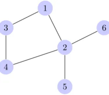
1 2 3 4 5 6
Figure 1: Network topology example used to illustrate the network discovery problem.
∀1≤i≤nPii= 0. (14)
Defining ON using P instead of A means that each of the rows in ON represents a boolean clause that we denote by α`, 1 ≤ ` ≤ mN (there are N time instants each producing a matrix with m rows). Consider the network in Fig. 1 as an example and assume that node 1 was infected and nodes 3, 4 and 5 are selected as sensors. The measurement y(0) = 03 has no information apart from the fact that the infected node is not one of the sensors making α1, α2 and α3 clauses with no information, i.e., the logical value of 1 (indeed this are removed by any solver). The measurement y(1) = e1allows to write α4, α5and α6 with some meaning. First, computing
CΦ(1, 0)x(0) = P13 P14 P15 , Φ(t, 0) := Pt+ Pt−1, (15)
determines that α4 = P13, α5 = ¬P14 and α6 = ¬P15, where the symbol ¬ stands for the logical negation. In doing so, the various clauses α`establish the set of possible instantiations for the variables Pij representing the existence or not of a link in the network.
The network discovery problem can then be cast as a Satisfiability Problem (SAT) in conjunctive normal form α1∧ α2∧ · · · ∧ αmN. The SAT problem has been extensively studied in the literature since it is one of the most well-known problems to belong to the class of NP-complete. Solvers are available such as
the one in [37]. SAT Competition 2016 reflects recent developments with certain experimental results, which contains statistical data showing SAT-VERIFIED or UNSAT and only returning one possible result once it is satisfiable, which means that the normal SAT solver has no guarantee of uniqueness. In our case, this might not be suitable as, due to the small number of constraints, the solver might simply return one of many possible assignments that could be meaningless to our problem. Algorithms returning sparse instantiations can be employed, using, for example, a memory efficient one that outputs all the possible solutions, see [38]. This solver returns the set of all the assignments to the important variables within certain constraints.
Besides the fact that the SAT problem is combinatorial by nature, and there-fore its complexity increases exponentially with the network size and number of clauses, requiring sparse solutions further adds to the complexity. Nevertheless, the SAT problem can be equivalently formulated as an optimization problem as: min P 1 s.t. A vec(P) >= β, Pii = 0, 1 ≤ i ≤ n, P = P|, Pij = 0 ∨ Pij= 1, i 6= j, (16)
where A is built from the α` variables by placing 1 if the corresponding Pij variable appears or −1 if it is its logical negation, β is a vector with entry i equal to one minus the number of times the ith variables appears negated and vec(P) is the vectorization operator applying only to the lower triangular part of P since P is symmetric. As an example, if there was only three clauses P14, P12∨ ¬P13 and ¬P23∨ ¬P12in a four node network, the constraint A vec(P) >= β would
be characterized by: 0 0 1 0 0 0 1 −1 0 0 0 0 −1 0 0 −1 0 0 P12 P13 P14 P23 P24 P34 >= 1 0 −1 . (17)
Remark that the optimization problem in Eq. (16) is just testing the feasi-bility of a solution and that the only source of non-convexity is the constraint that the entries in P are either zero or one. One of the common approach is to relax such assumption to the convex approach of 0 ≤ Pij ≤ 1. In particular, finding the sparsest network topology that is feasible can be expressed as the whole optimization problem
min P 1 | nP 1n s.t. A vec(P) >= β, Pii = 0, 1 ≤ i ≤ n, P = P|, 0 ≤ Pij≤ 1, i 6= j, (18)
which is convex and a linear program. Notice that we have not used the `1norm since all Pij >= 0 so there is no need to apply the absolute value operator and also because the norm would not ensure the sparsest solutions for cases where one of the nodes is fully connected (or is of higher degree than the rest).
5. Control of Infection Networks
In this section, we address the problem of how to control the infection net-work process (i.e., making it reach a desired state of infected or recovered nodes) and the related question of what is the optimal control to lead the network to a infection-free state.
5.1. Controllability analysis
The first question that should be answered is the condition for controllability of the system. Let us introduce the following definitions that are common in standard controllability theory. First the notion of controllability and reacha-bility subspaces. For the remaining of this section, matrix B(t) is a diagonal matrix with elements equal to one if that node can be injected with an infection or recovery. If all nodes are accessible, this is simply a identity matrix and the vector u(·) is added to the state.
Definition 5. Given two times instants t1 > t0 ≥ 0, the reachable subspace R[t0, t1] on the interval [t0, t1] consists of all states x1for which there exists an input sequence u(·) that transfers x(t0) = 0n to x(t1) = x1 in the DSIR model, i.e., R[t0, t1] := {x1∈ Rn: ∃u(·), x1= t1−1 X τ =t0 Φ(t1, τ + 1)B(τ )u(τ )}, (19) and the controllable subspace C[t0, t1] on the interval [t0, t1] consists of all states x0 for which there exists an input sequence u(·) that transfers x(t0) = x0 to x(t1) = 0 in the DSIR model, i.e.,
C[t0, t1] := {x0∈ Rn: ∃u(·), 0 = Φ(t1, t0)x0+ t1−1 X τ =t0 Φ(t1, τ + 1)B(τ )u(τ )}. (20)
Closely related are the concepts of gramians defined in the following. Definition 6. Given two times t1> t0≥ 0, the reachability and controllability gramians are defined as:
WR(t0, t1) := t1−1 X τ =t0 Φ(t1, τ + 1)B(τ )B(τ )|Φ(t1, τ + 1)| (21) WC(t0, t1) := t1−1 X τ =t0 Φ(t0, τ + 1)B(τ )B(τ )|Φ(t0, τ + 1)|. (22)
The controllability gramian assumes that the transition matrices are all non-singular. In our case, the objective is to apply these definitions to the underlying
linear system (i.e., without the bar operation) and extract conclusions regarding the nonlinear output. If one focused strictly on the traditional condition, it would mean that the system should be fully reachable (i.e., R[t0, t1] = Rn) whereas a milder condition might suffice. As an example consider a system whose state of the underlying linear part is always of the form x(t) = α
1 2
and we would like to make the desired infection state h1 1 i|
. Clearly any output leading to α > 0 would work since ∀α > 0 : x(t) =
1 1
but the system is not fully reachable.
Having introduced the required definitions, the next theorem summarizes both the reachability and controllability of the infection networks. The proof can be found in Appendix A.3.
Theorem 7. Given two time instants t1> t0≥ 0 and xtarget, the DSIR model can reach the observed state of xtarget if
∃x1: x1= xtarget, x1∈ R[t0, t1] = ImWR(t0, t1), (23) where ImWR(t0, t1) is the image (also called the column space) of WR(t0, t1), i.e., set of all linear combinations of vectors in the columns of the matrix. More-over, if the graph topology (V, E) is connected and t1− t0 ≥ d the infection network is controllable.
5.2. Optimal control strategy
In this section, the question of designing optimal control strategies for the network is addressed with respected to the energy of the control input. Resorting to the concepts reviewed in the last section, it is possible to provide the following result, proved in Appendix A.4.
energy u(·) for the DSIR model that can reach xtarget is given by: min x1 kB(t)|Φ(t1, t + 1)|η1k2 , s.t. x1= WR(t0, t1)η1, x1= xtarget (24)
where WR(t0, t1) is defined in Eq. (21), and the minimum norm to control the infection network using a single recovery at time t0to an observed state x1= 0n is given by: min u kuk2 s.t. Φ(t1, t0)x(t0) + Φ(t1, t0+ 1)u ≤ 0. (25) 6. Simulation Results
In this section, we provide simulation results both for the proposed general model to consider the source localization without prior knowledge of the initial time and also to the algorithm for network topology discovery. We then progress to present simulations showing the behavior of the infection network given the computation of the control law as proposed in this paper.
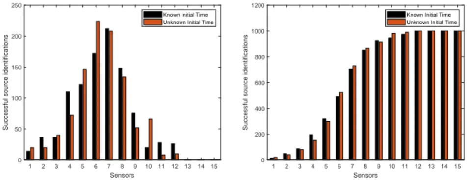
The first simulation compares the accuracy of the source localization with and without the knowledge of the initial time. The setup includes a randomly selected network topology with n = 100. The probability of including each link is set to 0.5 as to produce challenging examples, i.e., networks with lots of redun-dant paths from the source to the sensors. The source and an initial sensor are randomly selected following a uniform distribution. For each simulated model, the found source is compared with the actual case. If the identification is false, a new sensor is uniformly chosen from the remaining nodes. The experiment is reproduced in a 1000 Monte Carlo experiment and the aggregate successful recovery of the initial infection is presented in Fig. 2(a).
From the simulation results, a trend emerges that increasing the number of sensor nodes has a direct impact on the accuracy of the source localization.
1 2 3 4 5 6 7 8 9 10 11 12 13 14 15 Sensors 0 50 100 150 200 250
Successful source identifications
Known Initial Time Unknown Initial Time
1 2 3 4 5 6 7 8 9 10 11 12 13 14 15 Sensors 0 200 400 600 800 1000 1200
Successful source identifications
Known Initial Time Unknown Initial Time
Figure 2: Successful infection source localization for a 1000 Monte Carlo simulation as a function of the minimum number of sensors in the known and unknown initial time models (left) and the cumulative source identification (right).
This was expected as additional measurements place more constraints on the optimization problems reducing the ambiguity. From the cumulative plot in Figure 2(b), we can check the loss in performance due to the unknown initial time. For this simulation and under the prescribed conditions, both models had an 100% detection of the infection source albeit the unknown initial time represented a need for 2 more sensors to achieve that. This highly depends on the number of edges in the topology graph as more edges hinder the detection by adding redundant links from the source to the remaining nodes. Selecting a 0.5 probability of existing each edge led to the 100% detection. Simulations suggest that some networks have a large impact on the difference performance of the two models. One possible reason for this behavior is the additional ambiguity of not knowing the initial time.
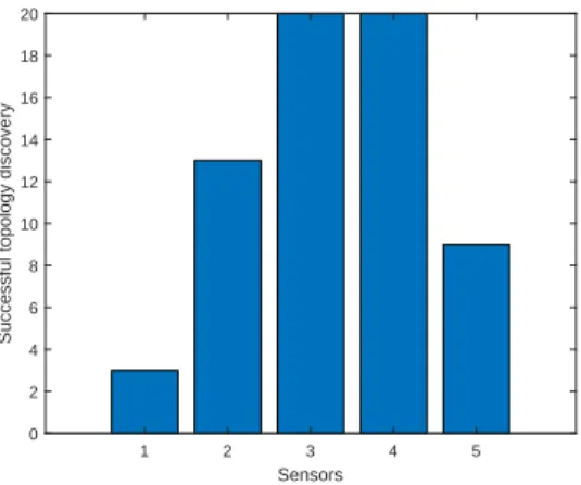
An algorithm to discover the network topology for the model with known initial information was also presented in this paper. In this setup, a 100 Monte Carlo simulation was conducted. In each run, a random topology of 5 nodes is selected with link probability equal to 0.5 along with a set of sensors selected randomly following an uniform distribution. The identification starts by inject-ing an infection in a random node and, if the output topology is different, a new infection is selected from the nodes not used previously in this run. The least number of sources needed before the network is correctly identified is shown in
1 2 3 4 5 Sensors 0 2 4 6 8 10 12 14 16 18 20
Successful topology discovery
Figure 3: Successful network topology identifications depending on the number of injected infections for 100 Monte Carlo experiment.
Figure 3. For the 100 cases, a 65% identification rate is reported with 55% of the identifications requiring half the number of nodes to be initially infected.
A critical key influence in the need to have 5 infection processes to half of the topologies is a consequence of the random network generations that is creating high-degree networks with nodes having on average half of the nodes as neigh-bors. The intuition behind this choice was that the best case scenario would be the path graph since the infection of one of the single-neighbors nodes would lead to detection as opposed to the complete network where n − 1 infections are required (in each infection process the solver learns that the current initial node is connected to all the others but no information regarding the connections between the remaining nodes).
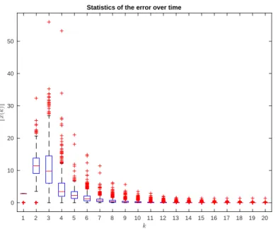
A topic also addressed in this paper was how one can apply control tech-niques made possible by rewriting the model as a Linear Time-Invariant (LTI) system with a nonlinear operation applied to the state giving the output. We simulated a random 8-node network where links between each pair of nodes have a 0.5 probability of existing. Three nodes are randomly selected to be the infected/recovered nodes. The optimal controller is found by resorting to the solution of the respective Discrete Algebraic Riccati Equation (DARE) us-ing R = I and Q = 10I. The state is initiated with all infected nodes, i.e.,
1 2 3 4 5 6 7 8 9 10 11 12 13 14 15 16 17 18 19 20 0 10 20 30 40 50
Statistics of the error over time
Figure 4: Statistics of the evolution of the error for an 8-node network with 3 controlled nodes and a 1000 Monte Carlo runs.
x(0) = 1n and the desired final state is x∞= 0n. During simulations, different configurations of the final state were tested and the behavior of the Monte Carlo experiment was always similar.
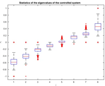
Figure 4 presents the statistics for the error norm, with each extremes of the box representing the first and third quantiles, the average being the line dividing the box and the extremes of the lines as the minimum and maximum. Crosses are presented for outliers of these distributions. In the vertical axis it is measured the norm of the error with respect to the evolution of the discrete time variable. We would like to point out that, contrary to what one might expect, in all instances the error first increases with the initial error being kx(0) − x∞k which in this case is √8. The typical errors after the 20 time instants of the simulation is on the order of 10−4 and a fast settling time as depicted in Fig. 4. In order to correctly picture the rate of convergence, we depict in Fig. 5 the statistics for each of the sorted 8 eigenvalues, i.e., the first box corresponds to the smallest eigenvalue in magnitude and the last box for the largest. On the vertical axis it is presented the value for the eigenvalues (real numbers with
1 2 3 4 5 6 7 8 -1 -0.8 -0.6 -0.4 -0.2 0 0.2 0.4 0.6 0.8 1
Statistics of the eigenvalues of the controlled system
Figure 5: Statistics for the sorted eigenvalues of the closed loop system after applying optimal control.
magnitude smaller or equal to one given that the dynamics is symmetric and stable) with respect to the i order of that eigenvalue, meaning that the first box is for the smallest eigenvalue and the last to the largest. The main point was to check the existence of some outliers runs where the spectral radius of the dynamics matrix is one and convergence is prevented. Such results motivate the use of the underneath linear model discussed in this paper since it rarely is the case.
7. Conclusions and Future Work
In this paper, we have presented an extension to the DSI model in its dynam-ical system view. In particular, without forcing the initial infection to happen at time equal to zero and allow an unknown time for the first infection. Such a modification, although reducing the accuracy of the source localization problem, increases the capability of this formulation to represent more advanced models. In addition, it is proposed a solution for the network topology discovery problem that is a convex relaxation of the integer programming approach to a traditional Satisfiability (SAT) problem.
In simulations, we have found evidence that suggests a loss in the localization success rate for the same number of sensors. The minimum number of sensor nodes before having a correct localization is smaller than or equal to half of the network in 60% of these random networks that are generated to have on average half of all possible links.
The last batch of simulations tested the network topology discovery algo-rithm based on a linear programming approach. For the considered model of the random networks, evidence suggests that half of the cases required 5 infec-tions processes to correctly identify the network.
Additionally, the problem of controlling the epidemics was tackled with a theoretical approach made possible by the design model where a linear system accounts for the evolution of the state whereas a nonlinear saturation opera-tion outputs the infected and recovered nodes. Standard techniques for linear systems were employed and shown in simulation to be very effective with fast settling times in achieving the final configuration of the infection network.
As directions of future work, two main trends can be pursued: use the gen-eral model framework to show how more evolved methods for infection networks can be simulated (for example stochastic models of infection); and, investigate algorithms to select the sequence of initial infections that render a faster net-work topology discovery. In addition, it is possible to consider the case where other information from distributed algorithms to further add restrictions to the network topology. In the latter, during simulations we have confirmed that the discovery time is highly dependent on the sequence of infections which motivates the future theoretical study. It would also constitute an interesting topic to fur-ther investigate if the identification of the source or topology of the network can be improved by adding other processes output or a priori information.
Researchers in the modeling community can also pursue extending the cur-rent underlying linear model to other alternatives in order to bring typical anal-ysis from those areas to relevant questions from infections networks. In this work, focus was primarily given to the control with minimum energy and local-ization, a natural extension would be to include the characteristic uncertainty
associated to infection processes by using other modeling alternatives like fuzzy models.
Acknowledgement 9. This work was partially supported by the project MYRG2016-00097-FST of the University of Macau; by the Portuguese Funda¸c˜ao para a Ciˆencia e a Tecnologia (FCT) through Institute for Systems and Robotics (ISR),
under Laboratory for Robotics and Engineering Systems (LARSyS) project UID/EEA/50009/2019. Carlos Silvestre is on leave from Instituto Superior T´ecnico, Universidade de
Lisboa, Lisboa, Portugal.
References
[1] A. Bauer, C. Beauchemin, and A. Perelson. Agent-based modeling of host–pathogen systems: The successes and challenges. Information Sci-ences, 179(10):1379 – 1389, 2009. ISSN 0020-0255. doi: https://doi.org/ 10.1016/j.ins.2008.11.012.
[2] E. Ferrara. Contagion dynamics of extremist propaganda in social networks. Information Sciences, 418-419:1 – 12, 2017. ISSN 0020-0255. doi: https: //doi.org/10.1016/j.ins.2017.07.030.
[3] S. Zejnilovi´c, J. Gomes, and B. Sinopoli. Network observability and local-ization of the source of diffusion based on a subset of nodes. In Conference on Communication, Control, and Computing (Allerton), pages 847–852, 2013. doi: 10.1109/Allerton.2013.6736613.
[4] M. Keeling and K. Eames. Networks and epidemic models. Journal of The Royal Society Interface, 2(4):295–307, 2005. ISSN 1742-5689. doi: 10.1098/rsif.2005.0051.
[5] J. Kephart and S. White. Directed-graph epidemiological models of com-puter viruses. In IEEE Comcom-puter Society Symposium on Research in Se-curity and Privacy, pages 343–359, 1991. doi: 10.1109/RISP.1991.130801.
[6] J. Kephart and S. White. Measuring and modeling computer virus preva-lence. In IEEE Computer Society Symposium on Research in Security and Privacy, pages 2–15, 1993. doi: 10.1109/RISP.1993.287647.
[7] D. Chakrabarti, Y. Wang, C. Wang, J. Leskovec, and C. Faloutsos. Epidemic thresholds in real networks. ACM Transactions on Informa-tion and Systems Security, 10(4):1:1–1:26, 2008. ISSN 1094-9224. doi: 10.1145/1284680.1284681.
[8] Y. Moreno, R. Pastor-Satorras, and A. Vespignani. Epidemic outbreaks in complex heterogeneous networks. The European Physical Journal B -Condensed Matter and Complex Systems, 26(4):521–529, 2002. ISSN 1434-6036. doi: 10.1140/epjb/e20020122.
[9] L. Allen. Some discrete-time SI, SIR, and SIS epidemic models. Mathe-matical Biosciences, 124(1):83 – 105, 1994. ISSN 0025-5564. doi: https: //doi.org/10.1016/0025-5564(94)90025-6.
[10] T. Tom´e and M. de Oliveira. Susceptible-infected-recovered and susceptible-exposed-infected models. Journal of Physics A Mathematical General, 44(9):095005, 2011. doi: 10.1088/1751-8113/44/9/095005. [11] J. Jacquez and C. Simon. The stochastic SI model with recruitment and
deaths I. comparison with the closed SIS model. Mathematical Biosciences, 117(1):77 – 125, 1993. ISSN 0025-5564. doi: https://doi.org/10.1016/ 0025-5564(93)90018-6.
[12] H. Khan, R. Mohapatra, K. Vajravelu, and S. Liao. The explicit se-ries solution of SIR and SIS epidemic models. Applied Mathematics and Computation, 215(2):653 – 669, 2009. ISSN 0096-3003. doi: https: //doi.org/10.1016/j.amc.2009.05.051.
[13] P. Mieghem. The N-intertwined SIS epidemic network model. Computing, 93(2):147–169, 2011. ISSN 1436-5057. doi: 10.1007/s00607-011-0155-y.
[14] P. Mieghem and E. Cator. Epidemics in networks with nodal self-infection and the epidemic threshold. Physics Review E, 86:016116, 2012. doi: 10. 1103/PhysRevE.86.016116.
[15] A. Ganesh, L. Massoulie, and D. Towsley. The effect of network topology on the spread of epidemics. In IEEE Joint Conference of the Computer and Communications Societies, volume 2, pages 1455–1466 vol. 2, 2005. doi: 10.1109/INFCOM.2005.1498374.
[16] S. G´omez, A. Arenas, J. Borge-Holthoefer, S. Meloni, and Y. Moreno. Discrete-time markov chain approach to contact-based disease spreading in complex networks. Europhysics Letters, 89(3):38009, 2010.
[17] P. Mieghem, J. Omic, and R. Kooij. Virus spread in networks. IEEE/ACM Transactions on Networking, 17(1):1–14, 2009. ISSN 1063-6692. doi: 10. 1109/TNET.2008.925623.
[18] N. Antulov-Fantulin, A. Lanˇci´c, H. ˇStefanˇci´c, and M. ˇSiki´c. FastSIR al-gorithm: A fast algorithm for the simulation of the epidemic spread in large networks by using the susceptible–infected–recovered compartment model. Information Sciences, 239:226 – 240, 2013. ISSN 0020-0255. doi: https://doi.org/10.1016/j.ins.2013.03.036.
[19] W. Guo, Q. Zhang, and L. Rong. A stochastic epidemic model with non-monotone incidence rate: Sufficient and necessary conditions for near-optimality. Information Sciences, 2018. ISSN 0020-0255. doi: https: //doi.org/10.1016/j.ins.2018.03.054.
[20] D. Hayden, Y. Chang, J. Goncalves, and C. Tomlin. Sparse network iden-tifiability via compressed sensing. Automatica, 68:9 – 17, 2016. ISSN 0005-1098. doi: https://doi.org/10.1016/j.automatica.2016.01.008.
[21] A. Seneviratne and V. Solo. Topology identification of a sparse dynamic network. In IEEE Conference on Decision and Control (CDC), pages 1518– 1523, 2012. doi: 10.1109/CDC.2012.6425980.
[22] B. Sanandaji, T. Vincent, and M. Wakin. Exact topology identification of large-scale interconnected dynamical systems from compressive obser-vations. In American Control Conference, pages 649–656, 2011. doi: 10.1109/ACC.2011.5990982.
[23] A. Chiuso and G. Pillonetto. A bayesian approach to sparse dynamic net-work identification. Automatica, 48(8):1553 – 1565, 2012. ISSN 0005-1098. doi: http://dx.doi.org/10.1016/j.automatica.2012.05.054.
[24] L. Zhao, W. Song, L. Tong, Y. Wu, and J. Yang. Topology identification in smart grid with limited measurements via convex optimization. In IEEE Innovative Smart Grid Technologies - Asia (ISGT ASIA), pages 803–808, 2014. doi: 10.1109/ISGT-Asia.2014.6873896.
[25] S. Bolognani, N. Bof, D. Michelotti, R. Muraro, and L. Schenato. Identifi-cation of power distribution network topology via voltage correlation analy-sis. In IEEE Conference on Decision and Control (CDC), pages 1659–1664, 2013. doi: 10.1109/CDC.2013.6760120.
[26] S. Huang, J. Li, J. Ye, A. Fleisher, K. Chen, T. Wu, E. Reiman, and t. Alzheimer’s Disease Neuroimaging Initiative. A sparse structure learn-ing algorithm for gaussian bayesian network identification from high-dimensional data. IEEE Transactions on Pattern Analysis and Machine Intelligence, 35(6):1328–1342, 2013. ISSN 0162-8828. doi: 10.1109/TPAMI. 2012.129.
[27] P. Pinto, P. Thiran, and M. Vetterli. Locating the source of diffusion in large-scale networks. Physical Review Letters, 109:068702, 2012. doi: 10.1103/PhysRevLett.109.068702.
[28] D. Shah and T. Zaman. Rumors in a network: Who’s the culprit? IEEE Transactions on Information Theory, 57(8):5163–5181, 2011. ISSN 0018-9448. doi: 10.1109/TIT.2011.2158885.
[29] B. Prakash, J. Vreeken, and C. Faloutsos. Spotting culprits in epidemics: How many and which ones? In IEEE International Conference on Data Mining, pages 11–20, 2012. doi: 10.1109/ICDM.2012.136.
[30] V. Fioriti and M. Chinnici. Predicting the sources of an outbreak with a spectral technique. arXiv e-prints, art. arXiv:1211.2333, 2012.
[31] E. Seo, P. Mohapatra, and T. Abdelzaher. Identifying rumors and their sources in social networks. In Proceedings of SPIE Defense, Security, and Sensing, volume 8389, pages 8389 – 8389 – 13, 2012. doi: 10.1117/12. 919823.
[32] D. Silvestre, P. Rosa, J. P. Hespanha, and C. Silvestre. Stochastic and deter-ministic fault detection for randomized gossip algorithms. Automatica, 78: 46 – 60, 2017. ISSN 0005-1098. doi: http://doi.org/10.1016/j.automatica. 2016.12.011.
[33] D. Silvestre, P. Rosa, J. P. Hespanha, and C. Silvestre. Finite-time av-erage consensus in a byzantine environment using set-valued observers. In American Control Conference (ACC), pages 3023–3028, 2014. doi: 10.1109/ACC.2014.6859426.
[34] D. Donoho. For most large underdetermined systems of linear equations the minimal l1-norm solution is also the sparsest solution. Communications on Pure and Applied Mathematics, 59(6):797–829, 2006. ISSN 1097-0312. doi: 10.1002/cpa.20132.
[35] H. Hao, D. Silvestre, and C. Silvestre. Source localization and network topology discovery in infection networks. In Chinese Control Conference (CCC), Wuhan, China., 2018.
[36] J. L¨ofberg. Yalmip : A toolbox for modeling and optimization in matlab. In In Proceedings of the CACSD Conference, Taipei, Taiwan, 2004. [37] SAT. SAT Competition 2016: Recent Developments, 2017. URL https:
[38] O. Grumberg, A. Schuster, and A. Yadgar. Memory Efficient All-Solutions SAT Solver and Its Application for Reachability Analysis, pages 275–289. Springer Berlin Heidelberg, Berlin, Heidelberg, 2004. ISBN 978-3-540-30494-4. doi: 10.1007/978-3-540-30494-4 20.
Appendix A. Proofs for the theorems in the paper Appendix A.1. Proof of Theorem 2
In this appendix we provide the proof for Theorem 2 found in Section 2. Theorem 2 (General Diffusion Susceptible-Infected (GDSI)). The DSI model in Eq. (4) without knowledge of the initial infection is equivalent to the dynamical system defined by the following equations:
z(t) = Φ(t, 0)z(0) + t−1 X τ =0 Φ(t, τ + 1)u(τ ) y(t) = Cz(t) ,
which can be rewritten as:
z(t) = t−1 X τ =0 Φ(t − τ − 1, 0)u(τ ) y(t) = Cz(t) .
Proof. In order to prove that the general diffusion model is given by Eq. (5), one has to show that Eq. (5) satisfies z(t) = x(t − tinitial), i.e., the general model is a shifted version of the model with known initial time where tinitial is the time where the infection was added in the general model.
Let us assume that indeed Eq. (5) is the state equation of the system. Then, it is possible to simplify it to the format:
z(t) = Φ(t, 0)z(0) + t−1 X τ =0 Φ(t, τ + 1)u(τ ) = t−1 X τ =0 Φ(t, τ + 1)u(τ )
= Φ(t, 1)u(0) + Φ(t, 2)u(1) + ... + Φ(t, t)u(t − 1),
where
Φ(t, tinitial) = At−tinitial+ At−tinitial−1. (A.2) In a simple SI, the infection signal u is defined as follows assuming node i is infected at time tinitial:
u(t) = ei t = tinitial 0n t 6= tinitial . (A.3)
Therefore, for any time t,
z(t) = Φ(t, 1)u(0) + Φ(t, 2)u(1) + ... + Φ(t, t)u(t − 1) = Φ(t, tinitial+ 1)u(tinitial),
(A.4)
or, equivalently,
z(t) = Φ(t − tinitial− 1, 0)u(tinitial), (A.5) by the properties of the transition matrix and thus obtaining that the model in Eq. (5) is equivalent to Eq. (6) and represents the standard model with a shifted time index of tinitialtime steps. Therefore, the transition matrix in Eq. (5) becomes
Φ(t, tinitial) = Φ(t − tinitial, 0), (A.6) and the conclusion follows.
Appendix A.2. Proof of Theorem 3
In this part of the appendix we present the proof for Theorem 3 found in Section 2.
Theorem 3 (DSIR model). The SIR model for a network of diameter d is equivalent to the dynamical system given in Eq. (5) provided that
u(t) = −1| nΦ(t + d, t)z(t)evt, if t ∈ T 0n, if t /∈ T
where vt is the infected/recovered node at time t. Moreover, Eq. (5) with Eq. (7) becomes: z(t) = Φ(t, ti1)ei1− X tτ∈T ti1<tτ≤t Φ(t, tτ+ 1)Θ(τ, d, Tτ)eτ,
where Θ(τ, d, Tτ) = X b∈Ψ(Tτ) |b|−1 Y ρ=1 (−1)|b|1|Φ(tρ+1+ d, tρ+ 1)eρ,
for Ψ(Tτ) being the set of 2τ −2 vectors with each vector being composed of the indices in Tτ for which there exists a one in the binary vectors of the form {1} × {0, 1}τ −2× {1}.
Proof. Two steps are required to prove this theorem, namely a) that selecting u as in Eq. (7) mimics a SIR model; b) that Eq. (5) with Eq. (7) results in the Eqs. (8)-(9).
a) In order for the system in Eq. (5) to mimic the SIR model, it is required that, at each time step after a new infection/recovery process, the only nodes that are affected are those with infected/recovered neighbors in the previous time instant.
Assume that node i is infected/recovered at time t from a process that started at time τ and node j, which is not a neighbor of i, is affected by i at time t + 1. Since i and j are not neighbors, it implies that the transition matrix in Eq. (5) has Φji(t + 1, τ + 1) = 0 but since node j was affected by i it implies Φji(t + 1, τ + 1) 6= 0, thus reaching a contradiction. Therefore, at most the process can propagate to the neighbors. Assume now the recovery (the converse for the infection follows the same reasoning) of node i at time t and a neighbor j that was not recovered at t + 1. This implies thatP
`∈Neighbors(j)z`(t) > |zi(t)|. However, by Eq. (7), |zi(t)| >P`6=iz`(t) >P`∈Neighbors(j)z`(t) resulting in a contradiction.
b) Given the state equation in Eq. (5), z(t) is a summation of transition matrices multiplied by −Θ(τ, d, Tτ)eτ for each event τ and constants Θ corre-spond to those defined in Eq. (7) (except in the initial infection when u = ei1).
Thus, gives the format in Eq. (8).
Notice that Eq. (7) defines u for the current infection/recovery at the ex-penses of the state at the previous events except for the initial infection. As a consequence, the input at event τ depends on all inputs up to τ − 1, forming
an unbalanced tree where each branch at the same level forks from zero to the number of current branches minus one (construction of the collection of vectors Ψ(Tτ)). Then, for each of the tree branches, a power of −1 is multiplied by the constant of the vector u as defined by the definition for vector u, giving the final expression for Eq. (9).
Appendix A.3. Proof of Theorem 7
In this subsection of the appendix it is presented the proof for Theorem 7 found in Section 5.
Theorem 7. Given two time instants t1> t0≥ 0 and xtarget, the DSIR model can reach the observed state of xtarget if
∃x1: x1= xtarget, x1∈ R[t0, t1] = ImWR(t0, t1),
where ImWR(t0, t1) is the image (also called the column space) of WR(t0, t1), i.e., set of all linear combinations of vectors in the columns of the matrix. More-over, if the graph topology (V, E) is connected and t1− t0 ≥ d the infection network is controllable.
Proof. The reachability result is a direct application of the reachability anal-ysis for linear time-varying systems with the difference that there must exist at least one state x1 in the underlying linear system that after the nonlinear operation returns xtarget as the observed state.
In order to prove the controllability, notice that if the network is connected, using Theorem 3 we know there exists an input that recovers all the nodes in at most the diameter of the network. Therefore, it implies that t1− t0≥ d, and the conclusion follows.
Appendix A.4. Proof of Theorem 8
Theorem 8. Given two time instants t1 > t0 ≥ 0 and xtarget, the minimum energy u(·) for the DSIR model that can reach xtarget is given by:
min x1 kB(t)|Φ(t 1, t + 1)|η1k2 , s.t. x1= WR(t0, t1)η1, x1= xtarget
where WR(t0, t1) is defined in Eq. (21), and the minimum norm to control the infection network using a single recovery at time t0to an observed state x1= 0n is given by:
min u kuk2
s.t. Φ(t1, t0)x(t0) + Φ(t1, t0+ 1)u ≤ 0.
Proof. The minimum energy for the reachability in Eq. (24) is an optimization ranging over all possible states x1 that generate xtarget as in Theorem 7. For each such state, standard reachability theory for linear systems allows to find the minimum energy path as that in the cost function in Eq. (24), and the conclusion follows.
Notice that given Theorem 7, one needs an input u such that after d time steps reaches the state 0n which implies that all entries i of xi(t1) ≤ 0. By minimizing the energy over all inputs that achieve the goal, the conclusion follows.