Optimal taxation rule on factor mobility: an application to the labor market case

• t

~. FUNDAÇÃO

~

#"

Getulio Vargas

EPGE

Escola de Pós-Graduação em Economia

Seminários

de Pesquisa

Econômica I (2

a

parte)

"OPTIMAL TAXATION BULE ON

F ACTOB MOBII,T-I-Y: Al\T

APPLlCATION TO TBI: LABOB

MABXET CASE"

j

JOSÉ CARLOS CARVALHO

----~~~- -~~-- --

-(Banco PactuaI)

.

~---~--~~~---~~--~

Fundação Getulio Vargas

,

ATA:

HORÁRIO:

Praia de Botafogo, 190 - 10

0

andar

Auditório

23/05/96

(53

feira)

16:00h

..

•

•

Optimal Taxation Rule on Factor MobUity:

An Application to the Labor Market Case

José Carlos Carvalho

I ..

Introduction

Our motivation to start studying labor market rigidity arose fiom the comparative observation of some different labor markets. Take the Brazilian labor market, for example. The Brazilian Payroll Survey (RAIS) indicates that in the eighties, on average, 30% of the existing job positions changed the tenured worker within a year. This means that every year 30% of the workforce moves fiom one job to another. On the overall, these jobs could be characterized as low-pay, low productivity jobs. On the other hand, we have the Japanese or European labor markets where labor relations between firms and employees are more stable. One can observe also that a typical worker in those markets is

better trained, what in turn yield a highly productive output. Comparing these two extreme positions one becomes extremely motivated to study some departures fiom the traditional mo deI that emphasizes that the maximum flexibility is the optimal outcome since it allows an optimal allocation of resources at every point in time. The two tables below present some sty1ized facts on the Brazilian and some selected OCDE labor markets.

Table I

Country Freqaency o, BaratAoo o, Country Frequency o, Baratlooo'

•

Unemployment Unemployment Unemployment Unemployment

• (1) (2) (1) (2)

..

Belgium 0.2 50 U.K • 0.9 10 France 0.6 21 Japan 0.5 3 Gumany 0.4 16 Norway 1.1 3 Jnland 0.7 30 Sweden 0.5 3 Jtaly 0.2 36 Spain 0.2 105 HoUand 0.4 25 Brazil(3) 2.5 1.6

(J)Data for 1988. The figure indicates the average number oftimes that a worker became unemployed in the year (2) Data for 1988. The figure indicates the average duraNon of unemployment in months.

(3) State ofSão Paulo only.

Source: Jackmon, Loyard and Nickell (1991)

Bivar (1993) for the Brazilian indicator - compatible methodology with JLN (1991) data.

TableH

Unemployment (%)

Source: ILO Yearbook

76- 86 87 88 89 90 91 91 93 94 95 85 Brazil 3.9 2.4 3.6 3.8 3.0 3.7 3.9 4.0 4.5

•

Japan 2.2 2.8 2.8 2.5 2.3 2.1 2.4 European Community 7.6 11.0 10.9 10.2 9.2 8.6 9.1 10.0 11.2 11.8 11.5

•

2

•

I

•

a

Tables I and

n

show that in Brazil the duration and the rate oflDlemployment are

smaIl and the frequency is high. lhese features suggest that the Brazilian labor market is

quite fleX1Dle. On the one side, tbis fleX1Dility is good because it propitiates an adequate

allocation of resources at every point in time. On the other hand, short term employment relations do not generate incentives for firms to invest in human capital, what implies in low-pay, low-productivity jobs. This last implication suggests that there is an optimal fleX1Dility in the labor market that is not the complete lDlconstrained movement of labor.

In fact, looking at the indicators for the European cOlDltries, one can obseIVe that the employment relations tend to be much more stable. lhe frequency of lDlemployment

is low, suggesting that firms operate with a stable workforce. This environment generates

incentives for the firm to invest in the human capital of their workers, and consequent1y these workers have high-productivity, high-pay jobs. lhe unfavorable outcome of this story is that the rate and duration oflDlemployment is very high. One ofthe arguments of

tbis paper suggests that this bad side might not be bad afier all if the increase in the labor market rigidity leads to an improvement in the general welfare.

lhe model developed in tbis article attempts to study the phenomena above and make some inference about welfare in the two extreme outcomes. We show that an increase in the labor market rigidity, lDlderstood as an increase in firing costs, leads to a increase in the number of workers that the firm keeps in a state of low demando This

explains why in the European case, where rigidities are higher, the frequency of lDlemployment is lower than in Brazil lhe effects on the average employment level however, is ambiguous. lhe increase in rigidity may lead to firms to hire more or less in

good times. It seems to be the case that in Europe this derivative is negative, since the duration ofthe lDlemployment and size oflDlemployment is quite high. In Japan, however,

I

•

•

the sigo. of this derivative seems to be positive, since a high stability of labor relations coexists with low unemployment and low duration ofunemployment.

Considering the worst seenario, in which high rigidities leads to high unemployment, we may ask if those economies are worse-off than in a scenario with less unemployment and less rigidity. In our last section we argue that this need not to be the case. We know that if there are externalities in the investment in human capital by the

firms, the private outcome leads to a sub-optimal social investment in human capital. In this case, the increase in the labor market rigidity is one way to bias the allocation towards the optimal central planner allocation -- what in tum increases welfare. This suggests that the environment ofhigh unemployment in Europe may still be better than a situation with

lower rigidities and more employment. Indeed, the higher rigidity led to a higher investment in training by the firms, and therefore it led to jobs with higher productivity and higher wages for the remaining workers. lhe government can tax the employed workers and pay generous welfare to unemployed workers and still make everyone better off Given the existence ofunobserved extemalities, the contnoution ofthis article is to derive a operational seheme that leads to an increase in welfare.

Afier this introduction, this article is divided into tive more sections. Section 11 takes a brief tour of the literature on the labor market rigidity. Section

m

develops a formal mo dei for the optimal private behavior of firms. Section N derives some comparative statics results from the solution obtained in Section

m.

Section V computes the private optimal value function derived from the private solution found in

m.

Finally section VI evaluates the welfare effects of an increase in firing costs .

I •

•

•

An important branch of the literature on labor market rigidity arose in recent years as a reaction to an earlier literature on the persistence of European unemployment. This

phenomenon was partly blamed on the labor market rigidities, specially high firing costs. lhe focus of this branch of the literature is, then, to show that more rigidity does not necessarily leads to more unemployment by itself

One important article in this area is the one by Bertola (1990). He finds that "Job security provisions alone cannot be blamed for the high unemplayment in European countries". He gets to this conclusion using 8 partia! equihorium analysis. Indeed, later on the article Bertola concedes that "Attention is focused on emplayment anti wage eflects: the welfare implications of different job security regimes (which appear ambiguous) are left to future research". This general welfare implic8tions is one ofthe points that we address in this article.

lhe positive aspect ofrigidity in Bertola's model arises from the fact that" .. .firms

tend to hire less in good times on/y because they rational/y expect to ( anti do) fire less in bad times. (. .. ) emplayment appears more stable and unemplayment more persistent in high job security countries, while no strong relationship emerges between job security

anti unemployment leveis." His conclusion, however depends strongly on the parameters

and the specific functional form adopted for the production function, as his maio. point is

that " .. . given functional forms and wage behavior,

if

r>O (interest rate), higher firing costs may tend to increase average emplayment even when higher hiring costs tend to

decrease it." This result is not proved for a generic case, but only for a numerical example for a set of parameter values and two different functional forms. lhe model is subject to

two different states of the nature. When choosing the parameters, Bertola sets them in such a way that " ... on average, good times last 5 periods, bad times 2.5 periods - rough/y

•

I

L __ _

realistic for business and product cycles." It seems that this specification could undermine a fair test of the effects of an increase in hiring and firing costs over employment. Since in good times the price increases by an E and in bad times they decrease by an E, the employment levei could be increasing simply because the real price

of the good sold by the firms is increasing through time.

Bertola & Bentolila (1990) folIows the same line of argument as Bertola (1990), except for assuming that the states of the nature (demand) are descnoed by a geometric Brownian motion (with a positive drift) instead of the discrete case ana1yzed in the previous paper. Again, the results are derived for numerical examples. According to the authors, "For realistic parameters values (which is a positive drift that implies a growth rate of demand of 2% per period in the stochastic process that descnoes the random shock) the size of the firing cost has practical/y no influence on average steady state labor demand. " 1

The authors further claim that, given the numeric parameters, " .. ..ftring costs prevent firing so much more than hiring that they increase the average unemployment. ". The explanation for this phenomenon is that "Asymmetric adjustment costs and a positive discount rate produce a ratchet elfect: the firm knows that (. .. )one day (. . .) firing costs wi/l have to be paid, but this possibility is heavi/y discounted since hiring occurs in good times, and bati times are far in the future. Expost, firing is less Iike/y to occur

if

firing costs are larger, and so average employment increases. "

1 When the authors try to get the result mentioned above assuming no drift in the demand shock, they simultaneously add the assumption that the rate of workers voluntarily leaving the finn is zero (pg.393). This assumption contributes strongly for their result, since it implies no change in the steady state levei of

employment by itself. In ali other simulations - where the drift is positive - the authors assume that a rate of 10% ofworkers leave the firm continuosly. The only case where this parameter is zero is when there is no drift in the Brownian motion.

"

&

•

m ..

Optimal Private Hiring and Firing Policies

lIl.1 .. lntroduction

The ultimate goal in this article is to develop a model in which an increase in labor market rigidity may lead to an improvement in welfare. In this section we start by detining a framework that characterizes the optimal private behavior of the firms. The model

considers the existence of two inputs (labor and training) and two states of the nature characterizing periods ofhigh and low demando The transition from one state to the other is descnl>ed by a Markov process that will be descnl>ed short1y.

The innovative feature of this model is to look at an increase in labor market

rigidity as an instrument to solve a problem of sub-optimal investment in training. We

assume that there are extemalities in the amount of training that firms give to their

workers. When investing in training, firms take into consideration only the direct eJIect

that this input has in their production. However there is a1so an extra eJIect on other firms

productivity that is not taken into consideration in the private solution. A central planner would obseIVe a social production function in which returns to training are greater than obseIVed by private firms. In this context, the private solution leads to a sub-optimal

investment in training. The next question, then, is how to induce private agents to mimic the optimal solution that would be adopted by a central planner. We aim to show that one

way to mimic the central planner solution might be to increase the firings costS .

•

•

The procedure descnbed in the previous paragraph aIIows us to address the issues of not only the employment evolution afier an increase in firing costs, but also the welfare effects of it .

IlI.2 .. A Formal Model

Firms maximize the present value of profuso They do so by choosing the optimal quantities of both inputs: labor and training. Adjustments in the labor force quantity are subject to some rigidities: Firms incur in both hiring and firing costs. Training has a once an for alI cost upon its acquisition -- and no extra cost. We assume that training is disembodied. In this sense, the acquisition of training can be seen broadly as the acquisition of knowledge or know-how. We descnbe below some more features of the model:

(a) There are two states of the nature that are characterized by the two prices that the good produced by the firms can assume:

(i) Good State - (High Demand) --> P,

=

Pg

(ü) Bad State - (Low Demand) --> P, = Pb

Obviously, the price in the good state is higher than the price in the bad state. But one further assumption is that the price variation between the two periods of the nature is such that the firms optimally choose to hire and dismiss workers when there is a change of

state. In other words, we are assuming that the change in price is such that the shadow price oflabor would go above the hiring costs ifno one were hired and it would go below the firing cost if no one were dismissed. 2 The alternative path could be one in which the

2 The implication of this proposition is that we need a lower bound for the price variation. The employment and training on both states ofthe nature are defined by equations (13)-(16) that are defined in

•

fluctuation was not enough to lead to hirings and :firings and therefore inaction would be the optimal policy for the firms. If this last case were true, however, any economic

analysis would be irrelevant. The graph below illustrates this point .

Hiring Cost

Firing Cost

Shadow Price PIth Leads

To Hirings and Firings

Graph I

Shadow Price PIth Leads

To Optimallnac:tion

Alternativa Plths for Shadow Price

(b) Prices follow a Markov process:

I~G,B~O.

(i) P[p,+1 = p₆

1p,

=

P_K] = G

P[Pt+l

=

pblp,

=

_PK] = (I-G) (ii) P[Pt+l

=

pblp,

=

Pb] = B

P[Pt+l

=

PKlp,

=

Pb] = (l-B)

We have argued before that a fair test of whether :firing COstS increase employment should be based in processes in which the likelihood of getting a good or bad state are equal.

This implies that G=B=1/2. Most of the time, though, we are going to work with a generic G and B in order to show that our resuhs do not depend on this feature.

11

-c

( e) State Variables:

(i) Nt = Total Number ofWorkers

(ü) Tt

=

Total Training (d) Control Variables:

(i) Ct = Flow ofworkers hired

(ü) Dt = Flow ofworkers fired

(iii) Yt = Flow oftraining hired

(iv) Xt = Flow of training dismissed

(e) Firms Maximize Profus. For a given time

s,

we have:

st: MAX {N,.T,.C,.D, .r,.x,}: ao V(.)

=

E,,"LP[Pt.F(Nt.1i.f)-w.Nt

-q.Y, -

_{H,Ct -F.Dt]} t=" N t

=

N t_1 +Ct - Dt

T,

=

T,-l

+

Y, -

Xt Ct ~ 0, Dt ~ 0,

Y,

~ 0, _{X t} ~ 0, _Nt ~ 0,

T,

~

°

N",Z;

given

From the problem above we ean set up the Lagrangean:

ao

"LP[Pt. F (Nt .1i. f )-w.Nt

-q.Y,

_{-H,Ct -F.Dt ]+} L(.)=E. t=:r

q ao ao

-"LP .1t·[ N t - Nt-1 -Ct +Dt]- "LP

.y,.[T, - T,-l

-Y,

+Xt ]

The Kuhn-Tueker maximum eonditions for the problem are:

(1) (2) (3) (4) (5) (6)

•

•

The set of equations above characterize the optimal solution for the problem

defined in (1)-(5). We show below the solution to this problem and prove that this

solution obeys the Kuhn-Tucker optimal conditions. The proof is actually divided into

two parts. The one presented below assumes that the initial points are the steady state values. On appendix 3 we show that starting from zero workers and zero training, the

economy converges to the steady state. The reason for splitting the proof into two parts is

that the convergence to the steady state leveI fol1ows a different path depending on

whether the first period is a good or bad period. One assumption underlying both the

proposition below and the one in the appendix 3 is that the price variation is above the

lower bound defined on footnote 2.

Proposition

-Then:

Let Ng, Nb, T*, y* be the solution to equations (13) to (16) below:

*

-P8.FN(Ng,T ,T) = w+H.(l-fi.G)+fi.F.(I-G) p" .FN (Nb, T*, f)

=

w - F.(l- fi.B) - fi.H.(I- B) P8· FT (Ng ,T* ,f)+fi.(l-G).y* = q.(I-fi·G) p".FT(Nb,T*, f)-y* .(1-{J.B) = -{J.(I- B).q N, =N₈ N, =N" 1'.

,

=

r

À=H

,

À

,

=-F y,

=q

15 V' t in which P I = P8 V' t in which Pt

=

p" V't V' t in which Pt = P8 V' t in which P t

=

P" V' t in which p t

=

P 8 (13) (14) (15) (16)

..

..

•

•

'v' t in which Pt =

P"

is a solution to the generic maximization problem defined by the Kuhn-Tucker maximum

conditions (7)-(12). Furthermore, the definition oí the state variables implied by the solution above determines a solution for the control variables. In the case of training, the solution above says that the amount of training is the same in both states. This implies that the flows oftraining are always zero, that is:

x=Y.=o

,

,

'v't

On the labor side, there are four posSlõle cases. lhe first one arises when the economy changes fiom a bad state to a good state. lhe optimal amount of labor in the bad state is Nb and in the good state it is Ng. In this case the flow is:

'v't in which Pt = P₈ and Pt-l = P"

lhe second case arises when the economy moves fiom a good to a bad state. In this case wehave:

{

C =0

D,

=~8-N"

'v't in which Pt = P" and Pt-l = P8

lhe third case occurs when two good states happen consecutively. In this case the optimal amount of labor is the same in both cases (Ng), what implies in no flow of workers, that is:

•

•

•

--- - ~--

-Finally, the same happens ifwe have two consecutive bad states.

In

this case we have:

We dedicate the following pages to show that the solution above satisfies the general equations of the prob1em defined by the first order conditions.

Proof

There are only two states of the nature characterized by the fact that the price leveI

is either pg or pb. We will show that the solution in Proposition 1 satisfies the general

Kuhn-Tucker maximum conditions (7)-( 12) in both cases.

When P, = P 8 the suggested solution asserts that the following is tme:

r,

=q

Note that since the shadow price oftraining is equal to 'q', the first order condition in (11)

will ho1d as an equality, what further implies that in the good state~. Another implication of y=q is that XG must be zero. This follow from the set of conditions in

(12). Therefore, in the good state it is not optimal to 100se anyamount oftraining .

•

If we move to the labor side, and considering that in the good state y=q, the first order condition in (9) becomes:

Â-, ~H

However, our solution claims that the equation above wiIl hold as an equality in the good state. This implies by (9) that CG~O. Also, since in the good state Â-G=H, we have from (10) that DG=O in the good state.

So far we have seen that the solution satisfies (9)-(12) in the good state. Now we check if it satisfies (7). If we substitute the suggested solution for the good state on the first order condition in (7), we have:

(17)

or rearranging some terms we have:

(18)

but according to equation (13) we know that the expression above hold as an identity, and therefore the set of conditions (7) is satisfied. Similarly, (8) would require:

Pg.FT(Ng,T* ,f)-q+P{G.q+(l-G).y*}

~

O (19)

..

(20)

but equation (14) guarantees that the solution holds the expression above with equality. Therefore in the good state our solution satisfies all equations of the general problem.

We now move to check that the solution is optimal in the bad state. In this case the

suggested solution is the following:

rI

=

r*

First, note that &ince the shadow price oftraining (y*) is a positive number, the first order condition in (12) holds as an inequality. This implies that XB has to be necessarily zero,

according to (12). Note that X had to be zero also in the good state. This implies that it

is never optimal to lose any training.3 _{Since X has to be zero in the bad state, the first}

order condition in (lO) becomes (in the bad state):

Our suggested solution implies that the equation above holds as an equality, what further

implies according to (10) that DB~O. Since À.B=-F, we know fiom (9) that C_{B has to be}

zero. Therefore we know that in both states it is not optimal to have firings and hirings at

the same time. If we go to the set of conditions (11), the fact that C B =0 implies that the first order condition will hold as an equality and therefore YB~'

3 This could be noted also from the fact that the shadow price of training is always positive. This follows from the fact that the shadow price of labor is given by the present value of the expected future marginal produtivity of training, which is always positive.

•

We can check that our solution a1so satisfies equation (7) in the bad state. In this case we have:

*

-p".FN(Nb,T ,T)-w+F+p.{B.(-F)+(1-B).(H)} ~ O (21)

or rearranging some terms we have:

(22)

equation (15) guarantees that our solution satisfies equation above with equality, what further implies that Nb;::1). Also, equation (8) a1so holds with equality. If we substitute our solution in equation (8):

p".FT(Nb,T* ,f)- y* +P{B.y* +(1-B).q}

~

O (23)

or rearranging some terms we have:

p".FT(Nb,T* ,f)- y*.(I-p.B)

~

-p.(I- B).q (24)

Equation (16) guarantees that the equation above holds with equality.

Therefore, we have shown that the solution above satisfies the equations of the

general problem for all periods of time. In the tables below we summarize the solution using the two equations of motion. Note that we use the notation ~ for the flow of workers. We will use this notation throughout the article for simplification.

•

Tablem

Summary of Optimal SoIution

Current Period is a Good State Curreot Period is a Bad State

Last Period was Last Period was Last Period was Last Period was

a Good State a Bad State aGoodState a Bad State

Nt Ng Ng Nb Nb Tt T* T* T* T* Ct O ~=(Ng-Nbl O O Dt O O ~=(Ng-Nb) O Yt O O O O Xt O O O O 111.3 -Investment in Training

One resuh from the general set of equations that characterize the Kuhn-Tucker

conditions for the problem above is that it is never optimal to discard the training input.

This follows from the fact that training has an once and for all cost upon its acquisition --and no further costs. Getting rid of training would imply a decrease in production -- since Ft>O -- and no savings in cost.

This can be seen also from the set of equations (12). If the firm is discarding some amount oftraining, this means that X>O and therefore this requires that yt=O. However, y

is the shadow price of training, which is the present value of the expected future marginal

productivities of training -- there are no extra costs afier its initiaI acquisition. This is

always a positive number. Since the shadow price is always a positive number, X has to

always be zero .

21

•

IV .. Firing Costs: Comparative Statics

In this section we advanee one more step in our goal to show that an increase in firing eosts may lead to an increase in welfare. Here, we take the private solution derived in the previous section, and analyze what is the optimal behavior for the firms conceming investment in training when faced by an increase in firing costs. Incidentally, we also

analyze what is the consequenee of an increase in firing eosts to the employment level

IV.1 .. Firing Costs and Investment in Training

The four variables that eharacterize the solution in our system are defined by equations (13) to (16). Note, however, that we ean substitute equation (16) in (15), eliminating y.. This allows us to work with a simplified system of three equations. We reproduee this modified system of equations below:

1::' ( • - ) p.(I-G) 1::' ( • - ) ( pG) p.(1-R) PK·rT Ng,T ,T

+

.p".rT Nb,T ,T = 1-. .q- .q (1- p.R) (1- p.R) (13) (14) (151 )

Our goal is to find the derivative of the private ehoiee of training (T*) with respect to firing eosts. If we totally differentiate the system above with respect to F, we have:

(15")

(13")

(14")

From equation (13") we have:

(13*)

From equation (14") we have:

(14*)

Now we ean plug (14*) and (13*) in (15") and get an expression for áT/dF as a function ofthe parameters only:

If we rearrange the terms in the expression above, the concavity condition for the

production function will appear:

Putting some terms in evidence, we have:

The concavity of the production function guarantees that:

•

To

simplifY

our notation, let's rename eaeh ofthese positive terms as:

{F1T(N B,T*,f).FNN (NB,T*, f)-[FNT (NB,T*,

nt }

= cI> > O

{F1T(NG ,T*,T).FNN (NG,T*,f)-[FNT(NG,T*,T)t}

=

'P

> O

Therefore we may re-write (13) as:

(29)

(30)

In order to infer the sign of dT*/dF, we ean obseIVe first that the denominator of expression (30) is always negative. This follows fiom the fact that both cI> and

'P

are positive and Fnn(.} is negative. Our goal is to show that an increase in firing eosts may lead to an increase in the amount of training purehased by the firm. In order to get

this

result the numerator must also be negative, that is, we must have:

(31)

Note that eaeh of the ratios above is negative, sinee Fnt>O and Fnn<O. Although not intuitive at first, the implieations of the assumption behind inequality (31) are very reasonable. It ean be interpret by looking at an iso-marginal productivity of labor curve, that is:

FN(N,T,T) = eonstant (32)

•

"

..

Taking the total differential ofthe expression above we have:

FNN(N,T,f).dN +FNT(N,T,f).dT=

o

dN FNT(N,T,f) = (33) dT FNN (N,T,f) Graphically we have: Good State N BacI Sate ---+---~---_T*

T

Graph II

Iso-Marginal Productivity cf Labor Curves

In the graph above we have two iso-marginal productivity of labor cwves. The slope of the cwves is positive, since we assume that these goods are complementary

(Fnt>O). Take any point in the cwve and increase vertically the amount of labor, without changing T. This will cause the marginal productivity on labor to fa1l (since Fnn<O). In order to keep it constant, we have to increase the amount of training (and this will do the job because Fnt>O). We may interpret the slope ofthis cwve as indicating the additional

•

•

productivity of labor eonstant. Our assumption just says that in the upper cwve (good state), when the firm has more workers, this additional amount oftraining is larger. Just to eheek that this equivalent to our assumption, we have just said that in the good state, á['ldN is bigger. But this is equivalent to say that in the good state, dNlá[' is smaller. Using our previous expression for dNlá[', we have:

(34)

Or, multiplying by minus one, we have the eonstraint we are imposing in the production function:

(35)

Therefore, if the production function is sueh that it obeys the technologieal constraint implied by (35), we may eonelude that the optimal reaction ofthe firms to an increase in firing eosts is to increase the investment in training.

IV.2 - Firing Costs and Employment levei

We ean now go baek to the system of three equations that eharacterize the solution and get some other eomparative staties resuhs. The first one is that an increase in firing eosts willlead to an increase in the number of employed workers in the periods of low demando This follows from equation (14*), reprodueed below for eonvenience. If we solve for dNbldF, we have:

•

•

(14*)

Note that dNb/dF is positive because both the denominator and the numerator ofthe ratio above are negative sinee Fnn<O and Fnt>O. The effect on the employment levei on the good state is ambiguous. This ean be ehecked by inspection of equation (13*), where

á.f*/dF is given by equation (30).

(13*)

The average employment levei may also rise depending on the magnitude of the parameters. The som ofthe employment on both states ofthe nature will go up if

(36)

Or, using (13*) and (14*), we have:

-{PB.FNT(NB.T •.

fl.~+(I-P.Bl}

+

{Ji(I-Gl-

PG.FNT(NG.,...Tl.~}

>0

PB·FNN (NB,T*,r) PG.FNN (NG,T*,r) (37)

..

•

-{(1-p.B)}

+ (P(l-G)} >0

PB·FNN (NB,T·,r) PG·FNN (NG,T·,'t) (38)

Or rearranging some terms, we have:

(39)

If the technical condition expressed by (39) holds, then the average employment of the economy will increase. This result does not depend on the fact that we have two inputs.

In fact, in appendix two we show that the average employment may indeed increase in a

similar model where labor is the only input.

v ..

The Optimal Value Function

This section is a necessary parenthesis in our presentation. It is dedicated to study the optimal value function that originates from the solution that we have found on section

m.

lhe reason to open this parenthesis is the need of a closed fonn for the optimal value function before we move into the study of the welfare implications of an increase in firing costs .

Anticipating some results in this section, the optimal value function will pOSSlOly assume four different values, depending on the current and past states of the nature. To understand this result, we start with Table N where the payoffs for the finn's optimal action in one period of time are shOWll. This payoff will depend on the present and the

..

past states of the nature. If the current state is good, and the previous one was bad, the

firm will have to incur in hiring costs. However, if the current state is good and the previous one was also good, the firm will no hire any more labor force -- therefore the hiring cost component is absent. Similarly, when the current state is bad, and the previous one was good, the firm will optimally adjust its labor force for the bad period optimallevel and will have to incur in firing costs. The same does not happen, however, if

the current period is bad, but the previous period was also bad. Since the previous period was bad, the firm enters the current period already with the optimal employment leveI for bad times, and therefore it will not incur in any firing costs in this case.

TABLEIV

t-l

t

Value Optimal Payolf at a Specific Time t

Good Good

_Vgg

V_u

=

P8·F (N₈,T,T)-w.N₈ Bati Good

Vbg

v,,8

=

P 8·F(N8,T* ,T) -w.N8 - H.A Good Bati

_Vgb

Vp

=

p".F(N",T*,T)-w.N" -F.A Bati Bati

_Vbb

V""

=

p".F(N",T,T)-w.N"

At each period in time, the optimal payoff will assume one out of the four possible values above. Therefore we can now move to the optimal value function, that is the

expected discounted present value of all optimal payoffs in the future -- as we defined the maximization problem on Section

m.

Since we are working with a symmetric problem, where the probabilities of each state of the nature happen are equal, we might be tempted to think, at first, that the optimal value function is the sum of each of the four possible payoffs weighted by 1/4. In fact, this is not the case. The reason for that is that the

and the possible payoffs in the subsequent period. Figure I below illustrates this problem. For example, if the current period is a bad state, there is no way that the 1irm wiD incur in firing costs next period -- this implies that Vgb wiD not occur for sure next period. We ean also see that neither wiD V gg. Therefore the fact that the current period is bad, narrows down the possibility for next period payoffto only two (S+ 1 in the figure below). From, the third period on (S+2 on the figure below), all four possibilities become equally

like1y. In Figure I we are using the fact that the probability of staying in the same state of the nature or moving to another state is 1/2. This simplifies the derivation of the optimal value function and implies that the shoeks are iid ..

5

Bad (Vbb) 5+1 Figure I 31 1/2 Good (Vgg) ...

Goo~

(Vgg)~

Bad (Vgb) ... 1/2 Bad (Vbb) ... Bad .-:;;:;--(Vgb)~ Good (Vbg) ... 1/2 Bad (Vbb) ...

Bad~

(Vbb)

~

Good (Vbg) ...

~

1/2 Good (Vgg) ... Goo (Vbg) 1/2 Bad (Vgb) ... 5+2 5+3

..

U sing Figure I above we can build the optimal value function for the case in which

the current state is a bad state. Note that there are two pOSSlole cases, since the current

payoffmaybe either Vbb or Vgb. Ifthe current period is Vgb, we have:

-

{lI}

/f

{I

1 l I }

V.r-b...r,( .. -l)_pod = V."

+p.

-'~8 +-.vw, + .

-.v

_u

+-.v."

+-.Vw, +-'~8 (41)

2 2 (l-fi) 4 4 4 4

Similarly, ifthe current state is a good state and the previous one was a bad state,

the optimal value function will be similar to the previous one, except for the first term:

-

{lI}

/f

{I

1 l I }

V.r=b...r,( .. -l).,ad = Vw,

+p.

-'~8 +-.vw, + .

-.v

_u

+-.v."

+-.Vw, +-'~8 (42)

2 2 (l-fi) 4 4 4 4

We have got above the two posSlole cases for the optimal value function if the current state is bad. We can do a similar exercise for the case in which the current state of

the nature is good. The tree below illustrates the pOSSloi1ities if the current state is a good state. Note that afier time (S+3), the payoffs are the same as the previous tree .

« •

5

Goo (Vgg) Bad (Vgb) 5+1 Figure 11

In this case, the two pOSSlole cases would be:

1/2 Good (Vgg)

Goo~

(Vgg)~

Bad (Vgb) 1/2 Bad (Vbb) Bad .-:;.:::;---(Vgb)~ Good (Vbg) 1/2 Bad (Vbb)

Bad~

(Vbb)

~

Good (Vbg) 1/2 Good (Vgg) Goo~ (Vbg)-m-- Bad (Vgb) 5+2 5+3

-

{lI} {I

1 l I } {I

1 l I }

Vr-,....,..-I)=,...., =VIlf +P -.vllf +-.v,. +{1. -.VIlf +-.V,. +-.v» +-.v. +f/. -.VIlf +-.v,. +-.v" +-.v. + ...

- 2 2 4 4 4 4 4 4 4 4

(45)

Similarly, if the current state is a good state and the previous ODe was a bad state, the optimal value functiOD wiIl be similar to the previous ODe, except for the first term:

(46)

Finally, we can summarize the four possible cases for the optimal value function in Table V below:

TABLE V

l-I I Value ofthe Optimal Value Function at Time t

Good Good

-

{lI}

_/f

{I

1 l I }

V

=

_{V +p. -Ygg +-Ygb}

+ - - .

_{- Ygg +-.Vgb +-.V}bb +-Ybg

gg

2 2

(l-fJ)

4 4 4 4

Bati Good

-

{lI}

_/f

{I

1 l I }

V

=

Vbg +p. "2 Ygg +"2 Ygb

+

(1-fJ)·

4

Y gg

+

4

Ygb +4"Ybb +4".Vbg

Good Bati

-

{lI}

_/f

{I

1 l I }

V

=

Vgb +p. -Ybg +-.V

2 2 (1-

bb

+ - - .

- Ygg +-Ygb +-Ybb +-.Vbg

fJ)

4 4 4 4

Bati Bati

-

{lI}

_/f

{I

1 l I }

V

=

Vbb +P -Ybg +-Y

2 2 (1-

bb

+ - - .

- Ygg +-Ygb +-Ybb +-Ybg

fJ)

4 4 4 4

Table V above relates the optimal payoffs per period (V) presented in Table IV

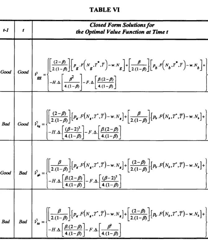
with the optimal value function (V). Ifwe plug the actua1 values ofthe payoffs that are given in Table IV, we can get closed form solutions for the optimal value functions. These closed form solutions are presented in Table

m

below. The calculations that lead us from Table V to Table VI are presented in the appendix I.

•

•

TABLE VI

Closed Form Solutions for

t-1 t _{the Optimal Value Function at Time t}

[2~~I-~J[P g.F(N g,T*,f )-W.N gJ+[2.(~fJ)J[Ph·F(Nh,T*,f )-w.Nh

J+

Good Good

_v

=

-H" [ ;-

]-Fâ

[1'(2-P>]

gg 4.(1-fJ) 4.(1-fJ)

[2~~1-!%

}[Pg.F(Ng,TO ,1')- W.Ng]+[ 2.(f-fJ) }[A.F(Nb,TO ,1')-w.Nb]+

Bati Good ~g=

-H.~.[

(/J-2i

]_F.~.[P.(2-fJ)]

4.(1-fJ)

4.(1-fJ)

[ P }[Pg.F(Ng,TO,1')-W.Ng]+[ (2-fJ) }[A.F(N,,,r,1')-w.N

b

]+

Good Bati

_V.,

=

2.(1- fJ)

2.(1-

fJ)

_H.~.[P.(2-fJ) ]-F.~.[

(/J-2)2]

4.(1- fJ)

4.(1- fi)

[ P }[P •. F(N.,TO,f)-W.N.]+[ (2-{J) }[A.F(Nb,TO,1')-W.N

b

]+

Bati Bati

_V

_bb

=

2.(1- fJ)

2.(1- fi)

_H.~.[P.(2-fi) ]-F.~.[

tf ]

4.(1- fi) 4.(1- fi)

Table VI is our primary to 01 to develop some analysis ofthe welfare implications of an increase in firing costs. This exercise is developed on the next section.

..

•

-- - -

-VI .. Welfare

On Section N, we have discussed some comparative static results that suggested that an increase in firing costs leads to an increase in the workforce in the bad state of the nature and also to a possible increase to the average employment levei Is the eventual decrease on the average employment levei necessarily a bad result? The point of this

section is to suggest that the measure for the adequacy of increasing firing costs should not be the increase in average employment levei -- even though this is an important indicator -- but the overall welfare. An increase in firing costs may lead to a distortion in prices that bias the private allocation towards the central planner solution -- and in this

case with extemalities in training, this solution is superior to the private one. This is independent of whether the average employment levei goes up or noto In other words, even with a decrease in the average employment leveI, the whole economy could be made better ofL This could he1p explain a caricature of the European outcome: High rigidities create lower average employment, but most of the remaining jobs are highly productive jobs. Those workers who remain employed benefit so much fiom the increased productivity that they are able to pay taxes that finance unemployment benefits for displaced workers. With this redistnõutive scheme, both groups could be made better 01f

than in an ahemative situation in which rigidities are low and jobs have lower quality.

The major departure fiom the material presented in the previous sections is the fact that in this section we use the "true" production function of the economy. As we have argued before, the investment in training has higher returns than those privately observed by the firms. Therefore, the private allocation is not optimal. A central planner, who can

•

,

function incorporating the true production function. Our exercise, then, is to evaluate the change in firing costs in the true optimal value function. We intend to show that it is pOSSll>le that an increase in firing costs leads to an allocation that yields a higher payoff in the true optimal value function than the original private solution.

Our first task is to define the function that the central planner would maximize. As

we have mentioned before, the maximization problem is similar to the one previously defined for the firms, except for the fact that the central planner does not consider T as given and maximizes with respect to this variable also. 4

00 MAX { N, .T,.i; .c, .D, .r, .x,

r

W(.)= E ..

LP[P,.F(N

_t,1(,ft)-w.N,

-q.Y,

-H.C,

-F.D,]

st.

T,=T,

N, = N'_l +C, - D,

T,

=

T,-l

+

Y, -

x,

c,

~ 0, D, ~ 0,

Y,

~ 0,

x,

~ 0, N, ~ 0,

T,

~

°

4 Note that tbis maxímization is similar to an welfare maximization if the constituents have an additive

utility function that depeneis on consumption and leisure. We can look at the objective function

ar

the central planner as the maxímization

ar

the net output (which is procluction discounted

ar

the real adjustment costs) plus leisure evaluated at the current wage rate.

In the problem above, (w. N ",n) is a constant. Therefore the maxímization problem becomes similar to

the maxímization problem for the firms, except for the fact that the central planner also maximizes with

respect to

T.

•

•

&

,

In fact, the central planner problem can be seen as being only to maximize the optimal value function of the private solution with respect to

T.

oS If the optimal value function of the private solution is given by

V

(F, T): 6

ao V(F,T)= MAX {N,.T, .c,.n, .r,,x,}; V(.)= ElILP[P,.F(Nt,1'r.T)-w.N,

-q.Y,

-H.C, -F.D,] st . N, = N'_1 +C, -D,

T,

=

T,-1

+

Y, -

X, C, ~ 0, D, ~ 0,

Y,

~ 0, X, ~ 0, N, ~ 0,

T,

~

°

Then we can write the optimal central planner value function, W(F), as a function ofthe private solution: W(F)

=

M4X V(F,T) T s.l. T

=

T(F,T) (49)

To solve the central planner problem, we have to maximize with respect to the one variable that was taken as a parameter before. Note also that the constraint implicitly

defines a function of T as a function of F -- since the private choice of training (1)

S In this case we are using the fact that:

MAX F(a,b)= MAX {G(a)= MAX F(b;a)}

d a b

6 After we solve for the endogenous variables. the optimal value function becomes a function of ali

•

•

•

depends on F and T =T. We ean plug this function T = T(F, T) into the objective function and work with an uneonstrained problem.

One important point to emphasize is the nature of the increase in firing costs. The govemment is artificially increasing the firing costs. This increase should be faced as a

tax, that generates resourees that are not 10st. The increase in firing eosts does not represent an increase in some inefficiency, that is, it is not the case that there are more resourees 10st in the eeonomy. Once we have this pool of resources originated by this

taxation, the next question is what is its destiny. We assume that the govemment pays baek its full amount in the form of a lump-sum payment every period for the firms

(independent of their actions). This lump-sum payment is set to equate the expected

revenue from this tax and the total payment for the firms.

Suppose that before the govemment intervention, the firing cost is

F'o

and afier it the firing eost rises to F. Therefore every time the firm tires workers, it will be paying an

extra (F-F'o) per worker. The expected present value ofthe taxation will be equal to the

expected present value of the rebate. Therefore we ean add one more eonstraint to the central planner maximization. The total expected tax revenue (T) originated by this

increase in firing costs is given by:

(50)

Note that the tax revenue above is expressed in present value. Therefore, the constant rebate per period (p) is defined as:

p= ,.(1-fJ) (51)

Or putting the two equations above together:

•

I

a

p = (1-

Pl.E,[

~P

(D,.

(F -

F,») ]

(52)

Therefore we may rewrite the central planner problem as: 7

W(F)=MF V(F,T)+r

st.

T

=

T(F,T)

T=

E,[~P(D,.(F

-

F,»)]

Therefore, the effect of an increase in the firing costs over the central planner optimal function can be expressed as: 8

(54)

Our task now is to find the sign ofthe derivative in equation (54). As a mst step, we verify that the last two terms cancel out. This is not swprising since there is no real increase in the inefficiency of the system. All the extra income taken from the firms is

completely paid back. The only difference is that the way it is paid back is designed to still

make firings more expensive.

7 Note that the priva te problem can be expressed as a particular case of this more general problem where there is no maximization with respect to

f

and F

=

F'o.

•

,

•

- -

-We can use Table VI and check that this is tIUe for each ofthe four possible cases that we have. Take the first case in Table VI.

An

increase in the firing costs wiD. cause a decrease in the optimal value function of:

v

={[2=f!LJ.[P.

J

N ,T·,'f)-W.N ]+[_P J.[Pb.

d

Nb'T·,'f)-W.NbJ-H.11.[~]-F.11.[P.(2-fJ)J}

gg 2.(1-fJ) g

'·l

g g 2.(1-fJ) ,.~

4.(1-fJ)

4.(1-fJ)

dV gg = {_L\.[P.(2-/3)]}

dF 4.(1-/3) (56)

Note that the derivative above is equal to the expected revenue ofthe tax imposed by the govemment. lhe expected tax revenue can be found with the he1p of Figure I in the previous section. Note that the firm only pays firing costs when the previous state was good and the current is bad (that is, Vgb in our notation). lherefore the expected income

18:

r=

P.{~

.L\.(F - Fo)}

+,lf.{

~

.L\.(F - Fo)}

+/f.{

~

.L\.(F - Fo)

}+/f.{~

.L\.(F - Fo)

}+ ...

Or:

r=p. -.L\.(F-Fo)

{I

}

+

{f

.

{I

-.L\.(F-Fo) =

}

p.(2-/3) .{L\.(F-Fo)}

2 (1-/3) 4 4.(1-/3)

From the equation above we can find the derivative dt/dF:

Notethat: dr =p.(2-/3).L\ dF 4.(1-/3) 41 (58) (59)

•

1

..

di dV

_u - + - - = 0 dF dF (60)

And therefore the last two terms of equation (54) cancel out. In this case, the govemment sets the rebate per period as:

(61)

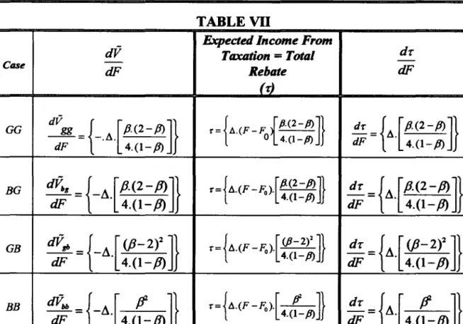
Clearly, the present value of the lump-sum payment equa1izes the expected income from the distortionary tax. The same resuh holds for the fom other cases. Table Vil below

summarizes the resuhs.

TABLE VII

dV

Expected lncome From _Taxation

₌

_Total

di

CllSe -

-dF Rebate dF

(i)

GG

dV

_{gg {}

[P(2-~]}

T=

{A.(F -F

{P.(2-/I)

J}

d,

+.[P.(2-~]}

dF = -.A. 4.(1-/1) o 4.(1-/1) dF 4.(1-P)

BG

dV;.

=

{ _A.[fi.<2 -

P> ]}

T={

_A.(F

-Fo).[!.~~=~]}

_dr

= {Ay"<2-P> ]}

dF 4.(1-/1) dF 4.(1-fJ)

GB

_{tiV ..}

= {-A.[

_{(jJ -}

2)' ]}

T={A.(F

-Fo).[

(P_2)1]}

_dr

={A.[

_(jJ-2)']}

dF 4.(1-/1) 4.(l-p) dF 4.(1-/1)

BB

tiV~

={-A [

_{fi' ]}}

T={A.(F

-Fo).[

ti ]}

_dr

={A [

_{fi' ]}}

dF . 4.(1-/1) 4.(I-P) dF . 4.(1-/1)

Considering that the rebate cancels out with the negative effect of an increase in firing costs on the optimal value function, we are then left with:

•

a

•

~(~) ~(~,~(F» ~(F)

tF

=

8I' .

----;n;:-

(62)

Note that the first term is always positive. The derivative of the optimal value function

with respect to T is just the derivative of the production function with respect to this variable. This wi11 always be positive, independent of the state of the nature. This fact is shown in the Table below:

TABLEvm

t-l t

_dV

~

Good Good

d;

=

{[

2(~;!

_].lpgFr(

N

g

,To

,r)]

+[

2(~ PJ].I

I'f,Fr(

Nh.r'

,r)]}

>

o

Bad Good

_{tIV ..}

={[

_(2-/f)

][PgFr(N,f,T)J+[

_P

][Pi.Fr(N,f,T)l}>o

dT 2.(I-P) 2.(I-P)

Good Bad

_tIV!'

_{r

_P

][PgFr(Ngf,T)J+[

_(2-/f)

][Pi.Fr(N,f,T)l}

_{> O}

dT 2.(1-P) 2.(I-P)

Bad Bad

d~

_{r

_P

][PgFr(Ngf,T)J+[

_(2-/f)

}[Pi.Fr(N,f,T)l}>o

dT 2.(I-P) 2.(I-P)

Since dV / dT >0 in alI four cases, the final welfare effect wi11 depend on the sign of

dT /dF on1y. The following pages discuss under what conditions this derivative is positive. We have found on section IV that under some technological constraints

I -

-I

I I

•

dT/dF>O. We discuss now the requirements for dT /dF to be also positive. The constraint to the central planner optimization is given by:

T = T(F,T) (63)

Ifwe differentiate the constraint with respect to F, we have:

8I' 8I' 8I' dT

+ =

-ôF 8I'. éF dF (64)

Or rearranging the terms, we have:

(65)

From the equation above we can see that the effect of an increase in the :firing costs on T and T wi1l be the same only if dT/dT is equal to zero. This follows from the fact that dT/dF is a partial derivative only. T is a function of both F and T. Therefore the

constraint implies that the total variation on T and T wi1l be the same but not necessarily the partial derivatives of these variables with respect to F. Indeed, if the T does not depend at all on T , what means that dT/dT is equal to zero, then both derivatives wi1l be identical. Since T and T are identical inputs, it is reasonable to assume that they are substitute goods, that is dT/dT

<o.

We discuss below the formal technological constraint for this to be true. If this is the case, and a1so the technological constraint that assures that dT/dF>O holds, then we have:

dT

dT =

di

>0

dF

[1-

:~J

I -

-I

I I

•

dT/dF>O. We discuss now the requirements for dT /dF to be also positive. The constraint to the central planner optimization is given by:

T = T(F,T) (63)

Ifwe differentiate the constraint with respect to F, we have:

8I' 8I' 8I' dT

+ =

-ôF 8I'. éF dF (64)

Or rearranging the terms, we have:

(65)

From the equation above we can see that the effect of an increase in the :firing costs on T and T wi1l be the same only if dT/dT is equal to zero. This follows from the fact that dT/dF is a partial derivative only. T is a function of both F and T. Therefore the

constraint implies that the total variation on T and T wi1l be the same but not necessarily the partial derivatives of these variables with respect to F. Indeed, if the T does not depend at all on T , what means that dT/dT is equal to zero, then both derivatives wi1l be identical. Since T and T are identical inputs, it is reasonable to assume that they are substitute goods, that is dT/dT

<o.

We discuss below the formal technological constraint for this to be true. If this is the case, and a1so the technological constraint that assures that dT/dF>O holds, then we have:

dT

dT =

di

>0

dF

[1-

:~J

(66)

..

•

From equation (68) we have:

(70)

From equation (69) we have:

(71)

Now we ean plug (70) and (71) in (67) and get an expression for ãI'/dF as a function of

the parameters only:

If we rearrange the terms in the expression above, the coneavity condition for the

•

•

Putting some terms in evidence, we have:

lhe concavity of the production function guarantees that:

To simplify our notation, let's rename each ofthese positive terms as:

{Frr(NB.T*.f).FNN (NB.T*.f)-[FNT(NB.T*.f)]l}

=

<I> > O

{Frr (NG' T*.f}.FNN (NG.T*.f)-[FNT(NG.T*.f)]l}

=

'I' > O

lherefore we may re-write (74) as:

47

(75)

PB·FNT(NB,T·,T) .p.(1-G). ar· .CI>+PG.FNT(NG,T.,T). ar·.'P+ FNN(NB,T·,T) (l-p.R) ar FNN(NG,T·,T) ar +p.(I-G). PB _{. {FTf(NB,T.,T).FNN (NB,T.,T)-}

FNT(NB,T.,T).FNT(NB,~,T)}+

(1- p.R) FNN (N B,T·,T) + PG _{_ .{FTf(NG,T.,T).FNN}

(NG,T.,T)-FNT(NG,T.,T).FNT(NG,~,T)}

=

o

FNN(NG,T·,T)

Ifwe name the two braeketed terms as:

e(N_B) = _{{FTf(NB,T.,T).FNN (NB,T·,T) - FNT(NB,T.,T).FNT(NB,T.,T)}} (78)

e(N_G) = _{{FTf(NG,T.,T).FNN (NG,T·,T)- FNT(NG,T.,T).FNT(NG,T·,T)}} (79)

We ean rewrite the equation above as:

(80)

The sign of dT*/dT will depend on the sign ofe. Note that ifboth e are positive then

dT·/dT will be negative as desired. So, the necessary eondition for dT*/dT to be negative is:

{FTf(·)·FNN (.)- FNT(·).FNf (·)} > O (81)

Note that FTf < O is a neeessary, but not sufficient, eondition for dT*/dT to be nega tive --assuming that F NT and _FNf have the same signo

..

•

If dT*/dT is negative, then according to (66) we know also that dT(F}(g, > O. Iftbis

is the case, then:

M(F) = óV(F,T(F». dT(F) > O

éF

õI'

dF (82)

That is, an increase in the firing costs may lead to an increase in welfare.

VII .. Conclusion

Afier finding that an increase in firing costs may induce an increase in welfare, one might be tempted to rename tbis article as "How Good is Eurosclerosis ... ". As we saw, the rigidity in the labor market caused by high firing costs may induce firms to invest more in the training of their permanent workers and also increase the number of permanent workers in the firm. We showed that, if the economy presents externalities in training, the allocation with higher firing costs might yield a higher welfare than the original private allocation. In this new allocation we have a higher net output per worker, what suggests that we can redistn"bute income from the permanent workers that have their position improved to those temporary workers that have their position worsened and make everyone better ofI Again, tbis seems to be the case in Europe, where generous unemployment benefits are paid to those displaced from their jobs. Contrasting with tbis situation, some labor markets in Latiu. America seem to be trapped in an equih"brium where the labor market is very fleXl"ble but with low qua1ity jobs. The ease to dismiss workers yields an equih"brium with toa many temporary workers and lower training.

Appendix One

Closed Form Solutions for the Optimal Value Function

The pwpose of this appendix is to find the closed form solutions to the optimal value functions on Table V using the optimal value for the payoffs presented in Table IV.

As a first step, we can see that all fom possible cases for the optimal value function look like the same afier the third period. Ifwe call this term

e,

we have:

(A 1. I)

We calculate the closed form solution for this common term first. Using Table IV, we

may r~write

e

as:

Or afier some algebra simplification, we have:

[f

{[

(

• -)

(

• -)

]

1l.(H+F)}

e=

.

_{P8.F N 8,T ,T +p".F N",T ,T -w.(N8+N,,) -} (A1.3)

2.(1-/1) 2

We now move to each ofthe fom particular cases:

a·

- - - - -- - - -

--Note that since the CUITent period is a good state, and coming fiom a good state, the firm

knows that it will not pay any adjustment cost this period. More than that, the fact that the firm knows that the CUITent state is good gives also the information that the following period must be V gb -- in which case the firm will pay some adjustment cost -- or V gg again. Working out the algebra and grouping the common terms, we have:

v

..

=

P_{Il .F(NIl ,TO}

,f).[I+!!.+

/f

]+

A,.F(Nb,TO ,

f). [!!.+

/f

]-W.NIl.[I+!!.+

/f

]+

2 2.(1-/1) 2 2.(1-/1) 2 2.(1-/1)

[ p

/f]

[/f]

[/f

P]

-w.N. -+ -H.A. -F.A.

+-b 2 2.(1-/1) 4.(1-/1) 4.(1-/1) 2

Or, afier some more algebra simplification we get the closed form solution for the first case:

Vu

={[

(2-/J) ]'[P •. F(N.,TO,T)-w.N.]+[

P

}[P".F(N",TO,T)-W.N,,]-H.t:..[

/f

]_F.t:..[ft(2-/J)]}

2(1-/J) 2(1-/J) 4. (l-/J) 4. (l-/J)

(b) Case TI: t-I =bad:t=good.

The procedure in this case is similar to the previous one. The only difference is in

the first period, since the CUITent period is a good state but the previous period was a bad

state. This change implies that it is optimal for the firm to adjust its employment levei to Ng. Therefore, it follows that in the CUITent period the firm will have to incur in hiring

costs. From Tables N and V, we have:

•

•

Working out the algebra and grouping the common terms, we have:

Or, afier some more algebra simplification we get the closed form solution for the second

case:

V_Ios

={[

(2-/1)

}[P •.

F(N.,TO,T)-W.N.]+[

P

].[P".F(N.,TO,T)-W.N.]-H.b..[

(P_2)1

]_F.b..[!;...P.~(2---,-/1),-,-]}

2.(1-/1) 2(1-/1) 4.(1-/1) 4.(1-/1)

(c) Case li: t-I=good:t=bad.

In this case, the current state is bad and the previous one was good. This implies that it is optimal for the firm to adjust to the employment leveI in bad times. This also implies that the firm will incur for sure i firing costs in the current período Using Tables N

and V, we have:

&

Or, afier some more algebra simplification we get the closed form solution for the third case:

- {[ P

I[

(

0-) ] [(2-/1)][ ( 0-) ] [P.(2-/1)]

[<P-

2

)1]}

V.,.

=

p •. F N.,T ,T -w.N. + . _{p".F Nb,T ,T -w.Nb -H.ll.} F.ll.

-2.(1-/1) 2(1-/1) 4.(1-/1) 4.(1-.8)

(d) Case ID: t-l =bad:t=bad.

Using Tables IV and V, we have:

Working out the algebra and grouping the common terms, we have:

!

P".F(Nb,T

O

,f).[I+!!..+

f!

]+Pg.F(Ng,TO,f).[!!..+

f!

_{]-W.Nb.[I+!!..+}

f!

]+1

_ 2 2.(1-/1) 2 2.(1-/1) 2 2.(1-/1)

V.

-bb -

-w.N

.[!!..+

f!

]-H.A.[!!..+ ti ]-F.A.[---"--ti ]

g 2 2.(1-/1) 2 4.(1-/1) 4.(1-/1)

Or, afier some more algebra simplification we get the closed form solution for the fourth case:

V/liI

={[

P ].[P •. F(N.,TO,T)-W.N.]+[ (2-/1)

}[P".F(Nb,TO,T)-W.Nb]-H.ll.[P.(2-/1)]-F.ll.[~]}

2(1-/1) 2.(1-/1) 4.(1-/1) 4.(1-/1)

-.

•

Appendix Two

Optimization Model with Labor Input Only

The pwpose of this section is to show that the average employment leveI may increase with an increase in firing costs even in a model in which there is only the labor ioput. In this case, the simplified mo deI is:

CIO

MAX V(.)= E .. LP[p,.F(Nt)-w.N, -H.C,-F.D, ]

s.t.

N ,

=

_{N I_1 +CI -DI} CI 2!: O, DI 2!: O, Nt 2!: O

No,

1'"

given

The Lagrangean is given by:

1=$

L(.)= E .. {i:P[P,.F(Nt)-W.N,-H.C,-F.D,]- i:P.Â,.[N, -NI_1-CI

+

D,J}(A2. 1

1 - I~

The first order conditions are given by:

E.[

~)]

=

p,.FN(N,)-w-

À, +p.E,[À,+,JS

O

N , 2!: O

N,.E,[

~)]

=

O

)