Repositório ISCTE-IUL
Deposited in Repositório ISCTE-IUL: 2019-03-26
Deposited version: Post-print
Peer-review status of attached file: Peer-reviewed
Citation for published item:
Baleia, J., Santana, P. & Barata, J. (2015). On exploiting haptic cues for self-supervised learning of depth-based robot navigation affordances. Journal of Intelligent and Robotic Systems. 80 (3), 455-474
Further information on publisher's website: 10.1007/s10846-015-0184-4
Publisher's copyright statement:
This is the peer reviewed version of the following article: Baleia, J., Santana, P. & Barata, J. (2015). On exploiting haptic cues for self-supervised learning of depth-based robot navigation affordances. Journal of Intelligent and Robotic Systems. 80 (3), 455-474, which has been published in final form at https://dx.doi.org/10.1007/s10846-015-0184-4. This article may be used for non-commercial purposes in accordance with the Publisher's Terms and Conditions for self-archiving.
Use policy
Creative Commons CC BY 4.0
The full-text may be used and/or reproduced, and given to third parties in any format or medium, without prior permission or charge, for personal research or study, educational, or not-for-profit purposes provided that:
• a full bibliographic reference is made to the original source • a link is made to the metadata record in the Repository • the full-text is not changed in any way
The full-text must not be sold in any format or medium without the formal permission of the copyright holders.
Serviços de Informação e Documentação, Instituto Universitário de Lisboa (ISCTE-IUL) Av. das Forças Armadas, Edifício II, 1649-026 Lisboa Portugal
Phone: +(351) 217 903 024 | e-mail: [email protected] https://repositorio.iscte-iul.pt
On Exploiting Haptic Cues for
Self-Supervised Learning of Depth-Based
Robot Navigation A↵ordances
Jos´e Baleia CTS-UNINOVA, Portugal Universidade Nova de Lisboa, Portugal
Pedro Santana
ISCTE - Instituto Universit´ario de Lisboa, Portugal Instituto de Telecomunica¸c˜oes, Portugal
[email protected] Jos´e Barata
CTS-UNINOVA, Portugal Universidade Nova de Lisboa, Portugal
Abstract
This article presents a method for online learning of robot navigation a↵or-dances from spatiotemporally correlated haptic and depth cues. The method allows the robot to incrementally learn which objects present in the environ-ment are actually traversable. This is a critical requireenviron-ment for any wheeled robot performing in natural environments, in which the inability to discern veg-etation from non-traversable obstacles frequently hampers terrain progression. A wheeled robot prototype was developed in order to experimentally validate the proposed method. The robot prototype obtains haptic and depth sensory feedback from a pan-tilt telescopic antenna and from a structured light sensor, respectively. With the presented method, the robot learns a mapping between objects’ descriptors, given the range data provided by the sensor, and objects’ sti↵ness, as estimated from the interaction between the antenna and the ob-ject. Learning confidence estimation is considered in order to progressively reduce the number of required physical interactions with acquainted objects. To raise the number of meaningful interactions per object under time pressure, the several segments of the object under analysis are prioritised according to a set of morphological criteria. Field trials show the ability of the robot to progressively learn which elements of the environment are traversable.
keywords: autonomous robots, self-supervised learning, a↵ordances, terrain assessment, depth sensing, tactile sensing
1
Introduction
The ability to safely navigate is as vital as complex for any useful embodied agent operating in natural environments. These environments exhibit high variability and the agent is subject to varying lighting conditions and noisy sensing. All these challenges compelled evolution to end up with agents capable of exploiting multi-modal sensory input. The same trend is typically followed by roboticists, which frequently find in sensor fusion a key element for a simultaneously robust and computationally parsimonious engineered solution. However, this path leads to high dimensional design spaces that can easily reach unmanageable complexity for the human designer. As a result, contemporary roboticists have turned to machine learning as an escape to this curse of dimensionality, which, nevertheless, brought its own challenges. How to teach these robots to make sense of their sensory feedback? Do we actually need to teach them, or they can learn by themselves?
In the context of safe navigation, the meaning that can be extracted from the sensory feed-back is completely grounded on motor actions. That is, the goal of perception in safe navigation is to determine which motor actions are feasible and, from these, which ones are optimal for the given task. To autonomously learn such perceptual skills, the agent needs to try out its motor actions repertoire in the environment and associate the outcome of these actions (e.g., did or did not overcome the obstacle) with the multi-modal appearance of the same environment. The incrementally acquired associative memory can then be used to estimate what motor actions are feasible in forthcoming interactions, given distal sensory feedback (e.g., visual). This self-supervised learning mechanism follows the a↵ordance prin-ciple studied by Gibson for the animal kingdom [14]. The concept of a↵ordances links the ability of a subject, through its actions, to the features of the environment and, so, to learn an a↵ordance the agent needs to interact with the environment.
Humans are known to be extremely good in the ability to learn a↵ordances, particularly because they can efficiently correlate visual and haptic cues [20, 37]. Following the same rationale, this article presents a method for the self-supervised learning of navigation a↵or-dances, given the outcome of haptic interactions between the robot and the environment. To this end, a wheeled robot is equipped with an active antenna for actively probing the objects present in the environment and check whether these are traversable or not by the robot. As the presence of vegetation in the environment is the most common cause of false obstacle detection, particular emphasis is herein given to vegetation sti↵ness assessment. The outcome of the antenna-object interaction process is associated with a descriptor of the object, which is computed from range data provided by a depth sensor fit to the robot. The resulting associative memory is used to classify subsequent objects imaged by the sensor. When these new objects look unfamiliar to the robot, new antenna-object interactions must be engaged. As interactions unfold, the robot’s associative memory grows and the need for physical interactions gets reduced. As a consequence of the learning process, the robot’s spatial reasoning look-ahead grows, thus fostering safer navigation.
With the proposed approach, the robot designer only needs to specify that the inability of the antenna to bend or trespass the object under analysis is a sufficient cue about the object’s
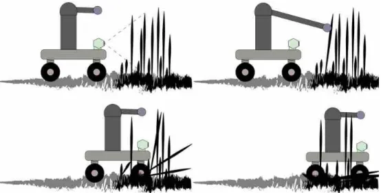
Figure 1: Proposed system’s major steps. (Top-Left) The robot finding an object with its depth sensor. (Top-Right) As the object’s class is still new to the robot, the latter physically interacts with so as to learn its traversability. (Bottom-Left) The robot overcoming the traversable object. (Bottom-Right) The robot determines that just finished crossing the object.
high sti↵ness and, hence, of not being traversable by the robot. This active perception [4, 1, 7] approach reduces considerably the design space when compared to one in which the traversable/non-traversable range-based classifier would have to be fully hand-crafted. This latter approach would also be surely less adaptive and, consequently, less robust in dynamic and unstructured environments. Fig. 1 depicts a caricature of the proposed method.
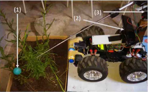
Fig. 2 depicts the wheeled robot prototype designed for experimental validation of the pro-posed method. The robot prototype is based on a 45 cm⇥ 35 cm ⇥ 65 cm 4-wheeled robot with di↵erential locomotion, fitted with a custom telescopic antenna with pan-tilt control. The antenna is capable of stretching up to 1 m and cover 180 degrees in both pan and tilt axes. The current drawn by the antenna’s servos is used by the robot to determine whether the antenna is blocked against a highly sti↵ object in the environment. This implements a form of proprioception.
As depth sensor, the robot uses a Microsoft Kinect, which employs modulated light to capture tridimensional point clouds of the environment. In a di↵erent context, this sensor has been shown to be able to acquire accurate enough 3D information for vegetation classification [3]. It is applicable robustly outdoors during the night and at most in the presence of dim daylight. For daylight operation the robot would have to be equipped, for instance, with a binocular vision sensor. As the noise model of these two sensory modalities is rather similar, the proposed model should be easily applicable to binocular vision and, as a result, enable daytime outdoors operation.
The system is implemented on the top of Robotics Operating System (ROS) [27] and relies on Point Cloud Library (PCL) [29] for low-level point clouds acquisition and processing.
Figure 2: The robot prototype with its antenna stretched to its maximum range. (1) Antenna tip (a rubber ball). (2) Depth Sensor frame of reference origin. (3) Antenna’s frame of reference origin.
This paper is an extended and improved version of a conference paper [6], and it is organised as follows. Section 3 describes the proposed system. Then, the results obtained from a set of field trials are presented in Section 4. Finally, a set of conclusions and future work avenues are given in Section 5.
2
Related Work
Robots are being applied to increasingly more demanding application domains in natural environments. Some outstanding examples include environmental and remote monitoring [10], support to search & rescue operations [26], humanitarian demining [31], patrol and reconnaissance [17], and agriculture [18].
To assess navigation cost in natural environments, a particularly difficult task given the lack of structure often found therein, these robots must rely on complex perceptual apparatus. Typically, the volumetric signature of obstacles is used for their detection from range data acquired by either laser scanners [8, 42, 39, 24] or binocular vision systems [22, 30, 34, 32]. Monocular appearance cues are also useful when exploiting known structures from the environment, such as the existence of paths to be followed [33, 28].
From all the challenges related to terrain navigation cost assessment, the ability to determine which objects are actually obstacles is possibly the most difficult one. For instance, vege-tation often generates volumetric signatures that can be confounded with non-traversable structures. To mitigate this problem, previous work analysed which descriptors computed from range data can be exploited to discriminate vegetation from other materials [21, 44].
In a parallel research thread, tree canopy characterisation from range data was also analysed [3, 25]. However, a binary vegetation / non-vegetation characterisation is a rather limited input for most robot control systems. For example, although grass and shrubs are both vegetated structures, only the former is traversable by small robots. Adds to this the fact that vegetated structures are highly heterogeneous, exhibit high intra-class variability, and change considerably from environment to environment. As a result, hand-crafting traversable / non-traversable robust decision heuristics is practically infeasible, as it is the production of significant hand-labelled ground-truth for supervised learning strategies.
The learning challenge for the problem of safe navigation in natural environments can be tackled by exploiting the fact that the goal is to learn visual categories that are grounded in the robot’s actions. That is, the robot needs to learn how to predict whether the object under analysis a↵ords a desired robot motor action. The most relevant a↵ordance in safe navigation is surely to be overcome. As in the a↵ordances framework the learning supervision signal is the outcome of the robot’s motor action, which is available for instance through proprioception, the learning process can proceed autonomously. This is essential as the robot needs to adapt its control system throughout its lifetime.
Self-supervised learning has been studied for load bearing estimation and obstacle detection in densely vegetated terrains from laser scans [43], as well as for cost assessment for terrain navigation from stereo vision [5] and overhead imagery [38, 16]. Traversability a↵ordances from laser scans for indoor robots were studied as well [41]. In all these cases, the robot learns what perceptual features better predict a given robot-terrain interaction, provided these can be measured by proprioception (e.g., collision detection, vibration sensing) while the robot traverses the environment. The associative mapping can then be used to predict the robot-terrain interaction, given sensory feedback from the far field obtained with distal sensors.
The need for the robot to traverse the environment in order to learn the corresponding environment-robot interaction can be harmful for either environment or robot and, hence, it is a limitation of the work described in the previous paragraph. In alternative, and inspired by previous work on learning of grasping and manipulation a↵ordances in humanoids (e.g., [9]), this paper proposes the use of a robotic antenna to perform the robot-environment interaction whenever learning about a given object’s traversability is required. The underlying idea is that the high controllability of the antenna-based interaction process ensures accuracy to the learning process and safety to both robot and environment. The goal is to learn how to infer from range data which objects in the robot’s field of view are bendable, i.e., traversable, by the robot.
Antennas and whiskers are interesting active sensing probes as these can exhibit high signal-to-noise ratio, are inexpensive, small, and provide low-bandwidth sensing. These properties of whiskers had led researchers to study their application to contact detection [12, 2], object recognition [36, 19], and surface texture discrimination [11].
Figure 3: Side (left) and front (right) views of the robot model with main frames of reference overlaid. (1) Locomotion system. (2) Depth sensor. (3) Robotic antenna.
3
The Proposed Method
3.1 Method’s Workflow
This section describes the proposed method, which aims at incrementally develop the ability to assess the cost of navigating in natural o↵-road environments. For this purpose, the robot learns a mapping between objects’ depth-based descriptors and objects’ sti↵ness.
Depth-based descriptors are computed from tridimensional (3D) point clouds of the sur-roundings, acquired by a depth sensor. The sti↵ness of objects is estimated by physically interacting with them with a small pan-tilt-telescopic controlled antenna. If throughout the physical interaction with the object the antenna gets stuck, which is verified by propriocep-tion, the object is said to be sti↵. Fig. 3 shows a schematic of the robot model and its main frames of reference.
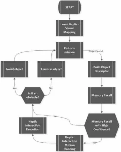
Fig. 4 depicts an overview of the method’s workflow. While executing a given mission, e.g., moving towards a specified waypoint, the robot may face an object. This object can be traversable (e.g., vegetation) or not (e.g., a rock). To assess it, the robot creates a depth-based descriptor of the found object and uses it to search its memory for the outcome of previous encounters with similar objects, themselves described using a depth-based descriptor of the same kind. If these previous encounters taught the robot that the object is traversable then the robot does not expend the e↵ort of avoiding it. However, while traversing the object the robot may find itself stuck and, consequently, needs to update the memory to report that the object is not traversable.
The more di↵erent the object faced by the robot is from the objects faced in previous encounters, the less confident the robot should be on classifying the object based on its memory. Bearing this in mind, in addition to classifying objects as either traversable or non-traversable, the method also produces a classification confidence level. Low confident classifications lead the robot to perform an haptic interaction with the object. The result of the interaction is then used to update the memory in terms of how traversable is the object. Moreover, the higher the confidence the robot has on the contents of its memory, the coarser
Figure 4: Proposed method’s workflow.
the haptic interaction must be. This allows the robot to reduce the time of interaction as the object gets known and, in the limit, when confidences rises to a certain level, the interaction is skipped altogether.
The next sections detail the several components required to implement the just described method’s workflow. Section 3.2 describes the procedure employed to learn the geometric mapping between the depth sensor and the antenna. The resulting mapping is consulted by the robot whenever it intends to reach the position of a 3D point described in the sensor’s frame of reference. Section 3.3 presents the object descriptor, which is the structure mem-orised when a new object is encountered and it is used whenever is necessary to perform subsequent object-object comparisons. These comparisons are memory recalling processes, which are described in Section 3.4. Whenever the system finds necessary to interact with the object, an interaction plan must be produced (see Section 3.5) and executed (see Sec-tion 3.6). Finally, the process employed to determine when the robot fully traversed the object, e.g., an extended grass field, is presented in Section 3.7.
3.2 Haptic-Visual Mapping
With only 3 degrees of freedom, the telescopic pan-tilt controlled antenna’s inverse-kinematics can be approximated with a simple tridimensional transformation from cartesian to polar coordinates. This transformation allows the antenna to reach a given tridimensional point in its workspace. These points are those determined as interesting in the tridimen-sional point cloud extracted from the depth sensor. A homogeneous point p = [x y z 1]T in
the robot’s workspace is described with respect to the antenna frame of reference, A, and sensor frame of reference, C, as
pA = [xAyAzA1]T, (1)
pC = [xCyCzC1]T. (2) Given the point coordinates in the camera frame of reference, the robot uses a 4⇥ 4 rigid body transformation matrix M to get the corresponding coordinates in the antenna’s frame of reference,
pA = MpC. (3)
To learn matrix M, the robot antenna performs a babbling behaviour in order to cover its configuration space. Simultaneously, the robot tracks the antenna’s tip with the depth sensor. This behaviour, which is engaged during an o✏ine calibration phase, allows the robot to accumulate a set of n correspondences between points in the antenna’s and in the sensor’s frames of reference,
pjA $ pjC,8j = 1, 2, . . . , n, (4) where a $ b represents a correspondence between point a and point b. Matrix M is estimated with a least-square SVD-based closed-form solution to the following minimisation problem [15]: arg min M ( n X j=1 ||pjA MpjC||2 ) . (5)
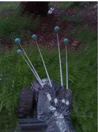
Fig. 5 shows a time lapse image of a typical babbling behaviour used by the system to calculate the several correspondences between points in the sensor and in the antenna frames of reference. Table 1 lists the several points in the antenna frame of reference considered for the exemplifying babbling behaviour.
To estimate the position of the antenna’s tip during the babbling behaviour, a background subtraction approach is used. First, the robot retracts its antenna so that it is surely away
Figure 5: Time lapse image of the babbling behaviour used to learn the rigid transformation between the range sensor and the antenna frames of reference.
from the sensor’s field of view and a reference 3D point cloud is acquired from the depth sensor. To reduce processing, only the 3D points that are within the antenna’s reach are considered in the following steps. This point cloud, which is representative of the background, is called reference point cloud. The reference point cloud feeds a reference octree for later processing.
The next steps are to stretch the antenna to the first position as defined by the babbling behaviour and acquire a new point cloud. This new point cloud already depicts the antenna overlaid on the background. To segment the foreground, that is, the antenna, the new point cloud is used to update the octree. All octree nodes that have been changed due to the introduction of the new point cloud are said to be the foreground, which includes antenna,
Point xA yA zA 1 -0.3 0.1 0.6 2 -0.3 0.2 0.6 3 0 0 0.8 4 0.1 0.1 0.8 5 -0.2 0.1 0.8
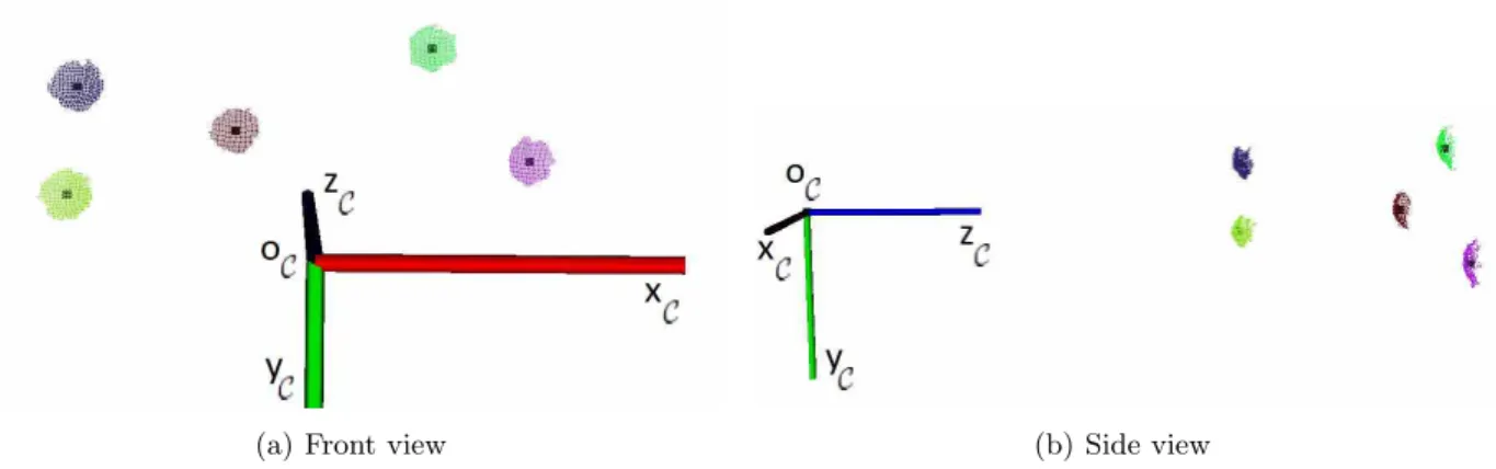
(a) Front view (b) Side view
Figure 6: Antenna’s tip corresponding segmented point clouds, as perceived throughout the babbling behaviour. The black dots inside the spheres represent their centroids.
noise, and moving background segments. Due to the materials employed in the antenna design, only the tip of the antenna is actually capable of properly reflecting the structured light pattern projected by the sensor. As a result, only the tip of the antenna is densely represented by the acquired point cloud. Nevertheless, other portions of the antenna, noise, and moving background segments are likely to be present as well.
To eliminate all 3D points that are not part of the antenna’s tip, a RANSAC [13] procedure is employed. Iteratively, RANSAC samples a minimal point set to generate a model hypothesis and then checks how many of the remaining points are explained by the model, i.e., are inliers of the model. The model hypothesis with highest number of inliers is picked as the final solution. As the antenna’s tip is spherical, the model herein estimated by RANSAC is the one of a sphere, which is represented by its radius and position in the sensor’s frame of reference. This method shows robust enough to discriminate between the antenna’s tip and other spurious point segments. This technique applied directly to the original point cloud, rather than to the foreground cloud, would be computationally more intensive. It would also be faultier in the presence of background segments whose shape could be mistakenly confused with the tip of the antenna.
Finally, the centroid of the points labelled as inliers by RANSAC is used as the antenna’s tip estimated position. Fig. 6 shows the antenna’s tip segmentation that results from the background subtraction process and application of the RANSAC procedure.
3.3 Object Descriptor
To ensure fast processing, the point cloud is down-sampled so as to ensure that no point is within a 1 cm radius of another point. This also counteracts the depth-dependent 3D point density variation imposed by perspective projection. Then, the object is segmented from the background by simply dropping all the 3D points that are out of the antenna’s reach. This is a sufficient strategy given the low vantage point of the robot’s sensor. Other configurations might require more complex object segmentation strategies. Finally, a descriptor of the object is built. The object’s descriptor will represent the object in memory and will be used for comparisons with other objects. It must be rich enough for a robust comparison but
simple enough for fast computations. Bearing this in mind, a set of four simple metrics based on a bidimensional histogram built from the 3D points distribution are considered. Let us assume that the optical axis of the depth sensor is aligned with the robot’s forward motion, i.e., parallel to the ground plane, and that the z-axis of the sensor is aligned with its optical axis, the y-axis is perpendicular to the ground plane pointing downwards, and the x-axis pointing to the right of the robot (see Fig. 3). The first step in building the descriptor is to project all 3D points onto a bidimensional histogram, H, coinciding with the sensor’s xy-plane. A bin in this histogram represents the number of 3D points that are encompassed by the parallelepiped that crosses the corresponding small squared region of the xy-plane and extends to the sensor’s maximum range.
The descriptor is based on a set of density and continuity metrics computed from the his-togram. This option follows from the assumption that the object’s sti↵ness is inferable from the object’s density and surface continuity. Intuitively, this assumption holds true for most situations in natural environments (e.g., tree trunk vs small bush). Moreover, density and continuity metrics are fast to compute. Let us call line to the set of histogram’s bins sharing the same y-coordinate. Let LH be the set of all lines present in histogram H. Let us call
cluster to a set of adjacent occupied bins, in a given line, that are separate from other clus-ters by empty bins. For a line l, the first metric is the number of clusclus-ters, nl. The second
metric corresponds to the number of bins found in the largest cluster, i.e., its size, sl. The
third metric is the point density, dl, which is computed by adding the number of points in
the line divided by the number of bins composing the same line. Finally, the fourth metric is the maximum number of points found in any of the clusters belonging to the line, ml.
Once the four metrics are computed for all the lines of histogram H, being these represented by the set LH, the j-dimensional descriptor of object o is built, j = 4|LH|,
{(no
l, sol, dol, mol),8l 2 LH}. (6)
3.4 Memory Recall
The memory is composed of descriptor-traversability tuples. A tuple associates the de-scriptor of the observed object and the traversable / non-traversable binary-valued outcome resulting from the physical interaction. In the current implementation, forgetting has not been implemented. Therefore, all interactions are stored and maintained throughout the robot’s lifecycle.
When facing an object, the robot will search for similar objects stored in memory in order to determine the most likely navigation cost of the object. This search demands for the ability to compute a dissimilarity metric between the descriptor of a just observed object, o, and the descriptor of any other object stored in memory, o0. This dissimilarity is computed based on local dissimilarity metrics, each one focused on a single element of the descriptor:
n(o, o0) = ✓ ⇣|no l no 0 l | ◆ , (7) s(o, o0) = ✓ |so l so 0 l | ◆ , (8) d(o, o0) = ✓ |do l do 0 l | do l ◆ , (9) m(o, o0) = ✓ |mo l mo 0 l | mo l ◆ , (10)
where ⇣, , , and are scale factors resulting from the sensor’s characteristics and typical object structure and (·) is a clamping function so as to ensure that the several metrics are within the interval [0, 1]. To compensate for the large variations that can be observed in the density of points and maximum number of points per cluster, the corresponding dissimilarity metrics exhibit a scaling division by do
l and mol, respectively. This scaling helps maintaining
fine comparisons between similar objects.
The four dissimilarity metrics are fused into a global dissimilarity metric:
(o, o0) = 1 4|LH|
X
8l2LH
✓
n(o, o0) + s(o, o0) + d(o, o0) + m(o, o0)
◆
. (11)
The simple recall of the most similar object stored in memory would be a brittle solution, as there is a high chance that noise has polluted the descriptor and the haptic interaction’s outcome of being an outlier. As a result, a k nearest neighbour approach is followed. The k nearest neighbours of the just observed object o are gathered in a set O and then segmented into two sub-sets. The sub-sets O+ and O correspond to the objects in O that have been
classified by the haptic interaction as traversable and non-traversable, respectively.
The average similarity between the observed object, o, and the objects stored in sub-set O+is
used to compute the level of confidence that the system holds on classifying o as traversable. Conversely, the average similarity between o and the objects stored in sub-set O is used to compute the level of confidence that the system holds on classifying o as non-traversable. Formally, the confidence levels associated with both traversable and non-traversable labels are: c+(o) = 1 k X o+2O+ ✓ 1 (o, o+) ◆ , (12) c (o) = 1 k X o 2O ✓ 1 (o, o ) ◆ . (13)
The label associated with the highest confidence level is the one used to classify the observed object o:
arg max
l2{+, }(c
l(o)). (14)
Finally, the confidence level on the object’s classification is the confidence level on the cor-responding label:
c(o) = max(c+(o), c (o)). (15) This confidence level serves the purpose of deciding whether the robot should traverse / avoid the object or, instead, physically interact with the object in order to improve its knowledge about it. The lower the confidence the higher the chances of engaging on a new haptic interaction.
3.5 Haptic Interaction Motion Planning
The position of each 3D point present in the point cloud is a candidate to contact point and, thus, a putative element of the motion plan. However, as most 3D points are redundant in terms of interaction results, a 3D point is only considered if farther than 5 cm from any other point already append to the motion plan. The points selected with this procedure are said to constitute a set P , need to be sorted according to a given objective function in order to become a useful motion plan.
The haptic interaction between the robotic antenna and the object under assessment should be as efficient as possible, otherwise it becomes time and energy over-consuming. In other words, the antenna’s motion plan should be short and highly directed towards highly in-formative contact points. Interacting with the leafs of a bush provides little information regarding the overall object’s sti↵ness. Conversely, hitting the main branch of the same bush will most probably block the antenna’s motion and, as a result, rapidly inform the robot that the object is non-traversable. Bearing this in mind, the ideal motion plan should be mostly composed of contact points located in the structural elements of the object, such as the main branch of a bush. Hopefully, right after the first iteration the robot gets to know what label must associate to the object’s descriptor.
The objective function applied to a given 3D point, candidate to the motion plan, p = (xC, yC, zC), with p 2 P , weighs three criteria. The first criterion builds from the intuition
that bending higher areas of the object (e.g., leafs) is usually easier than their lower areas (e.g., main branch). This intuition is formalised as a Gaussian function of the point’s height:
sh(p) = exp |yC
g|2
2· 2
!
where g is the sensor’s distance to the ground minus the height of the tallest traversable obstacle, given the robot’s kinematic characteristics, and an empirically defined scalar. The second criterion builds on the intuition that the object’s centroid should be the most dense and, thus, most difficult to bend. As a result, this criterion is defined as a Gaussian function of the distance from the point in question to the object’s centroid, c:
sc(p) = exp ||p
c||2
2· 2
!
. (17)
The third criterion is defined as the density of points in the neighbourhood of the position in question. The higher the density, the more likely the position is of belonging to the most difficult-to-bend object’s part. This criterion, sd(p), is computed by dividing the total
number of neighbours inside a predefined radius of the point in question, r. The total number of neighbours can be approximated as:
2⇡· r2
vw· vh
, (18)
where vw and vh correspond to the voxel width and height, respectively. This formulation
exploits the fact that the point cloud has been discretised into a regular grid, i.e., it has been voxelised.
Finally, the three criteria are combined in the objective function used to sort all points in the motion plan, p2 P :
s(p) = ✓h · sh(p) + ✓c· sc(p) + ✓d· sd(p), (19)
where ✓h + ✓c + ✓d = 1 are empirically defined scalars that would be ideally learned from
data.
Fig. 7 shows that points with score above 0.7, as computed with the objective function, do correspond to the portions of the object that are more likely to block the antenna. These points are located in the central and denser region of the object.
3.6 Haptic Interaction Plan Execution
Once the observed object is classified as traversable or non-traversable (Section 3.4), the classification confidence level is used to determine whether an haptic interaction is required. High confident memory recalls should result in low probable haptic interactions, as it is likely that the robot has learned sufficiently about the object in previous encounters. Conversely, if the memory recall is low confident, then the robot should interact with the object in order to learn more about it. This principle is implemented by exploiting the fact that the sequence of points to be analysed, i.e., the motion plan, is sorted by relevance (Equation 19).
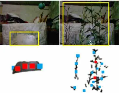
Figure 7: Typical interaction points suggested by the system as motion plan. Top row: input range images (only RGB information depicted). Yellow rectangles represent the regions containing the objects. Bottom row: segmented input range image. Red and blue filled squares represent the points with a score higher and lower than 0.7, respectively. Left column: a rock as representative of non-traversable objects. Right column: light vegetation as representative of traversable objects.
For a given observed object o, the confidence-based interaction depth, m, is controlled by pruning the already sorted set P . That is, only the m points with higher score (Equation 19) are selected for subsequent haptic interactions. The score threshold is defined as a proportion of the memory recall confidence level (Equation 15).
Formally, the set P is pruned as follows:
I = ⇢
pj, j 2 {1, . . . , m} , (20)
where j indexes pj in P and m is determined so that the following conditions is met:
s(pm 1) < ↵· c(o) ^ s(pm) > ↵· c(o), (21)
where ↵ is an empirically defined scalar controlling how cautious the system must be. With a high ↵, the system reduces the number of interaction points and favours past expe-riences, whereas a low ↵ increases the number of interactions, making the system to behave more cautiously. As a result, ↵ can be used by a higher-level reasoning system to adapt the speed-accuracy trade-o↵ exhibited by the system depending, for instance, on exogenous en-vironmental stress. Such a system would be following the rationale that haptic interactions are slower but more accurate than visual cues.
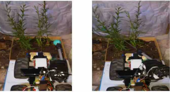
Figure 8: Typical haptic interaction execution. The antenna stretches to the distance of the furthest interaction point then follows the plan. Note that this behaviours results in a scanning pattern that bends traversable obstacles.
The motion plan being built, the robot proceeds with its execution. The plan execution starts by picking the robot-centric rightmost point in I and successively moving the antenna to the point in I that is closest to the previously picked one. This proceeds until all points have been scanned or the antenna gets blocked. In the latter case, the object is labeled as non-traversable and traversable otherwise.
To raise the chances of getting the antenna blocked due to the presence of a non-traversable object, the points to be reached are translated 5 cm along zC. The sweeping-like motion resulting from following the plan scans the environment in a way that the presence of non-traversable objects are likely to block the antenna motion. Fig. 8 and Fig. 9 depict such a typical haptic interaction. If, instead, the points were simply pushed by the antenna in a sequence, i.e., without employing a sweeping behaviour, the chances of slithering by the object would be rather high.
3.7 Environment Change Detection
If the object facing the robot is considered traversable, either via highly confident memory recall or via haptic interaction, the robot will try to traverse it. In some cases the object is in fact a large extension of vegetation which fills the sensor’s field of view while the robot traverses it. As a result, the robot faces recurrently the same object at each new progression step. To avoid recurrent traversability assessments and putative interactions with the same object, whose traversability was assessed at the onset of the progression, a mechanism to detect that the object is no longer present in the sensor’s field of view or that another object within the original object (e.g., a rock surrounded by vegetation) was found is required. Due to the robot’s small size, surrounding vegetation covers most of its sensor’s field of view.
Figure 9: A typical motion plan (sequence of arrows connecting thick dots) overlaid on supporting point cloud (thin dots).
Thus, the changes to be captured when the robot leaves the object are scene-wise. Scene-wise descriptors are often known as gist descriptors [40] and are rather useful in order to determine, for instance, when a given robot behaviour is appropriate, given the context of the current scene [35]. A scene’s reference gist is computed before the robot starts traversing the object. Then, at each progression step, a new point cloud is captured and its gist is compared with the reference gist. If this di↵erence is greater than an empirically defined scalar, !, then the robot may engage on a new interaction (e.g., check the rock found that is surrounded by vegetation).
A fast processing solution is herein proposed for the calculation of the gist descriptor from range images. First, the point cloud is reduced by superposing a regular grid on it. The centroids of the grid elements are taken as the reduced point cloud. Then, the number of points composing the original point cloud and the reduced point cloud are computed. The ratio between both quantities is the gist descriptor of the scene. This ratio describes, in a concise and fast to compute way, the average point density of the point cloud, which was found to be sufficient for the problem at hand.
As the implemented gist descriptors are scalars, comparing di↵erences between them is defined as the absolute di↵erence between their descriptors. If this di↵erence is greater that an empirically defined scalar, then the environment is assumed to have changed.
4
Experimental Results
4.1 System Parameterisation
The bidimensional histogram used as object descriptor has 16 ⇥ 14 bins, meaning that |LH| = 14 (Section 3.3). These dimensions shows a proper tradeo↵ between detail and
computational parsimony. Memory recall relies on a set of scale factors considered in local dissimilarity computation, ⇣, , , and (Equation 8-10), which were set to 0.5, 0.2, 2, and 2, respectively. These values were obtained from the geometry of the sensor and typical object’s characteristics. The number of neighbours considered in the memory recall process was set to k = 5.
Follows the parameterisation for the haptic interaction motion planning process (Section 3.5). For the point cloud simplification step, a voxel size of 4 cm3 was used. By taking into account
the robot’s morphology, the scalar g in Equation 16 and in Equations 16-17 were set to 0.1 and 0.8, respectively. To compute the interaction points sorting criteria (Equation 19), the scalars ✓h, ✓c, and ✓d, were set to 0.3, 0.2 and 0.5, respectively. These were picked by
observing the final score in a set of typical point clouds. The radius used to find the point neighbours in sd(·), r, was set to 0.1m.
Finally, a density change detection threshold of ! = 0.03 was set for the voxel size of 0.01 m3
(Section 3.7).
4.2 Classification Accuracy from Haptic Interactions
To assess the system’s classification accuracy based on haptic interactions, the robot was asked, in a controlled environment, to move forward until an object was found.
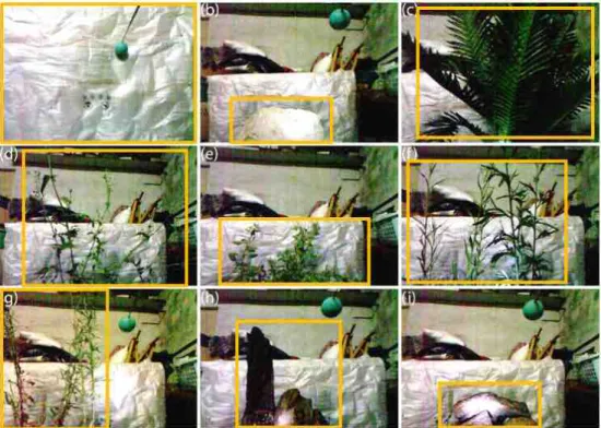
Throughout the process the robot faced 9 di↵erent objects, (a). . . (i), one at a time. Let us call these 9 objects data set 1. With each of them, the robot engaged on the haptic interaction process so as to determine whether the object is traversable or not. The set of objects includes four traversable plants, a non-traversable wall, a non-traversable plant, two piles of non-traversable logs, and a non-traversable rock (see Fig. 10). Fig. 11 shows the point clouds captured and haptic points suggested by the system.
Table 2 presents the number of interaction points in P within a given score interval (see Section 3.5) selected by the system for each tested object. The table shows that the number of points grows from higher scores to lower scores. This is consistent with the intuition that the good interaction points are fewer than the poor interaction points. Fig. 7 illustrates this phenomenon on a typical vegetated object. As expected, denser objects, such as logs and rocks, tend to exhibit a higher number of high scoring points than thin vegetation. For all objects, interacting with points with a score above 0.7 was enough to give a correct traversable / non-traversable classification.
Figure 10: Objects used for classification accuracy analysis in a controlled environment, as seen from the robot with its depth sensor. The yellow rectangles represent the objects’ bounding boxes. (a) Wall (non-traversable); (b) Rock (non-traversable); (c) Big plant (non-traversable); (d) Shrub (traversable); (e) Small shrub (traversable); (f) Tall plants (traversable); (g) Tall Plant (traversable); (h) Vertical logs (non-traversable); (i) Horizontal logs (non-traversable).
4.3 Classification Accuracy from Learning
To assess the robustness of the object descriptor (Section 3.3) and the memory recalling process (Section 3.4), a leave-one-out cross-validation analysis was undertaken based on the 9 objects. The principle used is to leave one of the objects out of the training set and then classify it based on the remaining training set, which has been hand-labelled. As depicted in Fig. 12, the system produced a correct traversable / non-traversable classification 67 % of the times for k = 1 and 78 % of the times for k = 3. This an interesting result given the lack of redundancy present in the data set. That is, for k = 3, the system recognises the objects based on their intra- and inter-class resemblance.
Score (a) (b) (c) (d) (e) (f) (g) (h) (i) [0.9, 1.0] 3 0 0 0 0 0 0 0 0 [0.7, 0.9[ 5 3 2 1 3 2 2 4 2 [0.5, 0.7[ 11 2 14 11 4 14 10 2 2
Figure 11: Object point clouds captured. The red points are the high-score interaction points suggested by the system.
To evaluate the ability of the system to incorporate new knowledge on the top of the 9 al-ready known objects, the robot was asked to travel towards two unseen objects (see Fig. 14). In a first test, the robot approaches the first object from various angles and for each ap-proach it tries to recall it from memory. The memory grows with the result of each of the new interactions. Fig. 13 shows that the system managed to recognise the object with a tendentially growing confidence as the number of interactions unfolded. The variability in the confidence level results from the fact that in each approach the object looked di↵erent to the robot - the object is anisotropic and the depth sensor is impinged with considerable noise. After 20 encounters with the first object, the robot was presented for the first time to the second object, which resulted in a low confident classification. As for the first object, the system managed to recognise the second object with a confidence level that tendentially grew with the number of encounters. Also as for the first object, the second object was approached from various angles. Let us call the several samples obtained from the novel two objects data set 2.
Let us now assume that the robot’s memory is filled with the samples from the two novel objects, i.e., data set 2. Let us also assume that the robot is unaware of the original 9 objects, i.e., data set 1. In this case the robot is said to be knowledgeable of an environment composed
Figure 12: Confusion matrix obtained from leave-one-out cross-validation.
Figure 13: Classification confidence plot corresponding to progressive acquaintance the episodic incorporating two new objects into memory. Typical classification confidence pro-gression. The two interrupted lines represent two piece-wise linear regressions of the confi-dence level before and after meeting the second object.
of objects contained in data set 2. In a real situation, when entering a new environment, the robot will progressively find new objects that must be capable of classifying and, potentially, integrate in its knowledge base. Table 3 shows that in most situations the robot is capable of properly classifying novel objects from data set 1 as traversable or non-traversable, given its prior knowledge about di↵erent objects from data set 2. This owes greatly to the redundancy in the appearance of objects in natural environments. Interestingly, erroneous classifications are also low confident, which forces the robot to interact with its haptic actuator to carefully assess the actual navigation a↵ordances of the object.
Figure 14: Novel traversable (top) and non-traversable (bottom) learned objects, and re-spective point cloud histogram.
4.4 Haptic Interaction Plan Execution
Low classification confidence compels the robot to engage on haptic interactions so as to robustly classify the object as traversable or non-traversable. The lower the confidence the higher the number of haptic interactions are engaged. This relationship is scaled by an empirical scalar ↵ (see Section 3.6). To provide some intuition about the parameterisation of this scalar, Fig. 15 shows its e↵ect on the number of haptic interactions while Table 4 shows the associated confidence levels after each encounter. The plot was built by varying the number of samples provided to the robot of object 1 from data set 2. This variation emulates the e↵ect of learning from various interactions. The higher the number of samples in memory the higher the confidence on the classification and, hence, the fewer the required haptic interactions. The figure also shows that the higher the value of ↵ the more the system values memory over haptic interactions. As expected, ↵ shows itself as a good modulator for the speed-accuracy trade-o↵.
4.5 Environment Change Detection
To avoid repeating haptic interactions while traversing a given object, the robot deter-mines an environment density change before reconsidering a new haptic interaction (see Section 3.7). Fig. 16 depicts three objects used to assess this capability with a density change detection threshold of ! = 0.03, while the voxel size used was 0.01 m3. For this
ob-Object Traversable Confidence Classification (a) No 0.42 Not Traversable (b) No 0.37 Traversable (c) No 0.33 Not Traversable (d) Yes 0.65 Traversable (e) Yes 0.48 Traversable (f) Yes 0.49 Traversable (g) Yes 0.60 Traversable (h) No 0.44 Traversable (i) No 0.23 Traversable
Table 3: Classification of objects in data set 1 given knowledge about objects in data set 2 with k = 5. Mis-classified objects: (b), (h), and (i).
Figure 15: Impact of di↵erent ↵ on the number of haptic interactions.
ject, performs a haptic classification, which returned traversable for all cases, and then tries to traverse the object. While doing it, the robot evaluates periodically if an environment density change occurred. If it occurs the robot stops and performs a new haptic verification. Two situations were studied for object A. In the first situation, A-1, the robot met open space when leaving the object, whereas in the second situation, A-2, the robot met an introduced wall-like object. In both situations the robot detected the density change, i.e., from object to open safe and from object to wall. When traversing object B the robot got stuck hampering it from progressing across the object. Correctly, the system remained without reporting any environment density change. As the robot gets stuck it becomes clear that the object is non-traversable despite did not look like it in the first haptic interaction. Corrective measures should be triggered correspondingly. Object C o↵ered no difficulties to the robot resulting in a fast traversal and easy change detection. These results are summarised in Table 5 and they show that environment density is a simple yet e↵ective metric for change detection in the context of object traversal.
Memory position Confidence Level Classification 6 0.38 Traversable 10 0.54 Traversable 13 0.57 Traversable 16 0.64 Traversable 18 0.67 Traversable
Table 4: Confidence levels and systems guess between same object encounters.
Figure 16: Objects used for environment change detection tests. (A) Small shrub; (B) Flimsy canes; (C) Twigs with thin leaves.
Object 1st 2nd 3rd 4th Change Detected A-1 0.019 0.013 0.014 0.055 Yes A-2 0.011 0.009 0.021 0.031 Yes B 0.020 0.018 0.008 - No C 0.014 0.059 - - Yes Table 5: Environment density change detection results.
5
Conclusion
A method for online learning of robot navigation a↵ordances from spatiotemporal correlated haptic and depth cues was presented. The method was implemented on a wheeled robot prototype and validated on a set of field trials. The results show that the method allows the robot to incrementally learn how to determine which objects present in the environment are actually traversable, most often vegetation. For the acquisition of haptic cues the robot relies on a low-cost pan-tilt telescopic antenna, whereas for distal sensory feedback the robot uses a low-cost depth sensor. Despite not being limited to this sensing apparatus, the system’s simplicity o↵ers a solution to small sized robots, which are useful tools for domains like environmental monitoring and search & rescue. These domain applications require from robots the ability to cope with the unstructured configuration of natural environments. This challenge is mitigated by the incremental learning of perceptual skills ensured by the proposed method.
Currently, we are assessing alternative depth descriptors, machine learning mechanisms, and haptic motion planning and execution policies. We are also studying how the method can learn its parameters o✏ine from real and synthetic datasets. The method is also being migrated to the medium-sized all-terrain robotic platform INTROBOT [23]. This robot is equipped with stereo vision, a tilting laser scanner, and a 6-DOF robotic arm, thus posing new challenges to the proposed method.
Acknowledgements
This work was co-funded by ROBOSAMPLER project (LISBOA-01-0202-FEDER-024961). We would like to thank Eduardo Pinto for his contributions to the design of the robotic prototype.
References
[1] Aloimonos, J., Weiss, I., Bandyopadhyay, A.: Active vision. International Journal of Computer Vision 1(4), 333–356 (1988)
[2] Anderson, S.R., Pearson, M.J., Pipe, A., Prescott, T., Dean, P., Porrill, J.: Adaptive cancelation of self-generated sensory signals in a whisking robot. IEEE Transactions on Robotics 26(6), 1065–1076 (2010)
[3] Azzari, G., Goulden, M.L., Rusu, R.B.: Rapid characterization of vegetation structure with a microsoft kinect sensor. Sensors 13(2), 2384–2398 (2013)
[4] Bajcsy, R.: Active perception. Proceedings of the IEEE 76(8), 996–1005 (1988)
[5] Bajracharya, M., Howard, A., Matthies, L.H., Tang, B., Turmon, M.: Autonomous o↵-road navigation with end-to-end learning for the lagr program. Journal of Field Robotics 26(1), 3–25 (2009)
[6] Baleia, J., Santana, P., Barata, J.: Self-supervised learning of depth-based navigation a↵ordances from haptic cues. In: Proceedings of the IEEE International Conference on Autonomous Robot Systems and Competitions (ICARSC), pp. 146–151. IEEE (2014) [7] Ballard, D.H.: Animate vision. Artificial Intelligence 48(1), 57–86 (1991)
[8] Batavia, P., Singh, S.: Obstacle detection in smooth high curvature terrain. In: Pro-ceedings of the IEEE International Conference on Robotics and Automation (ICRA), pp. 3062–3067. IEEE Press, Piscataway (2002)
[9] Detry, R., Baseski, E., Popovic, M., Touati, Y., Kruger, N., Kroemer, O., Peters, J., Piater, J.: Learning object-specific grasp a↵ordance densities. In: Proceedings of the IEEE International Conference on Development and Learning, pp. 1–7 (2009)
[10] Dunbabin, M., Marques, L.: Robots for environmental monitoring: Significant advance-ments and applications. Robotics & Automation Magazine, IEEE 19(1), 24–39 (2012) [11] Fend, M.: Whisker-based texture discrimination on a mobile robot. In: Advances in
Artificial Life, pp. 302–311. Springer (2005)
[12] Fend, M., Bovet, S., Pfeifer, R.: On the influence of morphology of tactile sensors for behavior and control. Robotics and Autonomous Systems 54(8), 686–695 (2006)
[13] Fischler, M.A., Bolles, R.C.: Random sample consensus: a paradigm for model fitting with applications to image analysis and automated cartography. Communications of the ACM 24(6), 381–395 (1981)
[14] Gibson, J.: The concept of a↵ordances. Perceiving, acting, and knowing pp. 67–82 (1977)
[15] Haralick, R.M., Joo, H., Lee, D., Zhuang, S., Vaidya, V.G., Kim, M.B.: Pose estimation from corresponding point data. IEEE Transactions on Systems, Man and Cybernetics 19(6), 1426–1446 (1989)
[16] Heidarsson, H., Sukhatme, G.: Obstacle detection from overhead imagery using self-supervised learning for autonomous surface vehicles. In: Proceedings of the IEEE/RSJ International Conference on Intelligent Robots and Systems (IROS), pp. 3160–3165. IEEE (2011)
[17] Huntsberger, T., Aghazarian, H., Howard, A., Trotz, D.: Stereo vision–based navigation for autonomous surface vessels. Journal of Field Robotics 28(1), 3–18 (2011)
[18] Johnson, D., Naffin, D., Puhalla, J., Sanchez, J., Wellington, C.: Development and implementation of a team of robotic tractors for autonomous peat moss harvesting. Journal of Field Robotics 26(6-7), 549–571 (2009)
[19] Kim, D., M¨oller, R.: Biomimetic whiskers for shape recognition. Robotics and Au-tonomous Systems 55(3), 229–243 (2007)
[20] Lacey, S., Hall, J., Sathian, K.: Are surface properties integrated into visuohaptic object representations? European Journal of Neuroscience 31(10), 1882–1888 (2010)
[21] Lalonde, J.F., Vandapel, N., Huber, D.F., Hebert, M.: Natural terrain classification using three-dimensional ladar data for ground robot mobility. Journal of field robotics 23(10), 839–861 (2006)
[22] Manduchi, R., Castano, A., Talukder, A., Matthies, L.: Obstacle detection and terrain classification for autonomous o↵-road navigation. Autonomous Robots 18(1), 81–102 (2005)
[23] Marques, F., Santana, P., Guedes, M., Pinto, E., Louren¸co, A., Barata, J.: Online self-reconfigurable robot navigation in heterogeneous environments. In: Proceedings of the IEEE International Symposium on Industrial Electronics (ISIE), pp. 1–6. IEEE, IEEE (2013)
[24] Montemerlo, M., Becker, J., Bhat, S., Dahlkamp, H., Dolgov, D., Ettinger, S., Haehnel, D., Hilden, T., Ho↵mann, G., Huhnke, B., et al.: Junior: The stanford entry in the urban challenge. Journal of field Robotics 25(9), 569–597 (2008)
[25] Moorthy, I., Miller, J.R., Berni, J.A.J., Zarco-Tejada, P., Hu, B., Chen, J.: Field char-acterization of olive (Olea europaea l.) tree crown architecture using terrestrial laser scanning data. Agricultural and Forest Meteorology 151(2), 204–214 (2011)
[26] Murphy, R., Stover, S.: Rescue robots for mudslides: A descriptive study of the 2005 La Conchita mudslide response. Journal of Field Robotics 25(1-2), 3–16 (2008)
[27] Quigley, M., Conley, K., Gerkey, B., Faust, J., Foote, T., Leibs, J., Wheeler, R., Ng, A.Y.: Ros: an open-source robot operating system. In: Proceedings of the IEEE ICRA Workshop on Open Source Software, vol. 3, pp. 1–6 (2009)
[28] Rasmussen, C., Lu, Y., Kocamaz, M.: A trail-following robot which uses appearance and structural cues. In: Field and Service Robotics, pp. 265–279. Springer (2014) [29] Rusu, R., Cousins, S.: 3d is here: Point cloud library (pcl). In: Proceedings of the IEEE
International Conference on Robotics and Automation (ICRA), pp. 1–4 (2011)
[30] Rusu, R., Sundaresan, A., Morisset, B., Hauser, K., Agrawal, M., Latombe, J., Beetz, M.: Leaving Flatland: Efficient real-time three-dimensional perception and motion plan-ning. Journal of Field Robotics 26(10), 841–862 (2009)
[31] Santana, P., Barata, J., Correia, L.: Sustainable robots for humanitarian demining. International Journal of Advanced Robotics Systems 4(2), 207–218 (2007)
[32] Santana, P., Correia, L.: Swarm cognition on o↵-road autonomous robots. Swarm Intelligence 5(1), 45–72 (2011)
[33] Santana, P., Correia, L., Mendon¸ca, R., Alves, N., Barata, J.: Tracking natural trails with swarm-based visual saliency. Journal of Field Robotics 30(1), 64–86 (2013) [34] Santana, P., Guedes, M., Correia, L., Barata, J.: Stereo-based all-terrain obstacle
de-tection using visual saliency. Journal of Field Robotics 28(2), 241–263 (2011)
[35] Santana, P., Santos, C., Cha´ınho, D., Correia, L., Barata, J.: Predicting a↵ordances from gist. Proceedings of the International Conference on the Simulation of Adaptive Behavior (SAB) pp. 325–334 (2010)
[36] Scholz, G.R., Rahn, C.D.: Profile sensing with an actuated whisker. IEEE Transactions on Robotics and Automation 20(1), 124–127 (2004)
[37] Schwenkler, J.: Do things look the way they feel? Analysis 73(1), 86–96 (2013)
[38] Silver, D., Sofman, B., Vandapel, N., Bagnell, J.A., Stentz, A.: Experimental analysis of overhead data processing to support long range navigation. In: Proceedings of the IEEE/RSJ International Conference on Intelligent Robots and Systems (IROS), pp. 2443–2450. IEEE (2006)
[39] Thrun, S., Montemerlo, M., Dahlkamp, H., Stavens, D., Aron, A., Diebel, J., Fong, P., Gale, J., Halpenny, M., Ho↵mann, G., Lau, K., Oakley, C., Palatucci, M., Pratt, V., Stang, P., Strohband, S., Dupont, C., Jendrossek, L.E., Koelen, C., Markey, C., Rummel, C., van Niekerk, J., Jensen, E., Alessandrini, P., Bradski, G., Davies, B., Ettinger, S., Kaehler, A., Nefian, A., Mahoney, P.: Stanley: The robot that won the darpa grand challenge. Journal of Field Robotics 23(9), 661–692 (2006)
[40] Torralba, A., Murphy, K.P., Freeman, W.T., Rubin, M.A.: Context-based vision system for place and object recognition. In: Proceedings of the IEEE International Conference on Computer Vision (ICCV), pp. 273–280. IEEE Computer Society, Washington, DC (2003)
[41] U˘gur, E., S¸ahin, E.: Traversability: A case study for learning and perceiving a↵ordances in robots. Adaptive Behavior 18(3-4), 258–284 (2010)
[42] Urmson, C., Ragusa, C., Ray, D., Anhalt, J., Bartz, D., Galatali, T., Gutierrez, A., Johnston, J., Harbaugh, S., Kato, H., Messner, W., Miller, N., Peterson, K., Smith, B., Snider, J., Spiker, S., Ziglar, J., Whittaker, W., Clark, M., Koon, P., Mosher, A., Struble, J.: A robust approach to high-speed navigation for unrehearsed desert terrain. Journal of Field Robotics 23(8), 467–508 (2006)
[43] Wellington, C., Courville, A., Stentz, A.T.: A generative model of terrain for au-tonomous navigation in vegetation. The International Journal of Robotics Research 25(12), 1287–1304 (2006)
[44] Wurm, K.M., Kretzschmar, H., K¨ummerle, R., Stachniss, C., Burgard, W.: Identi-fying vegetation from laser data in structured outdoor environments. Robotics and Autonomous Systems 62(5), 675–684 (2012)