SOCIUS Working Papers
Horácio C. Faustino
Maria João Kaizeler
Do Lottery Sales Differ Across Income Classes Becoming An Inferior Good For Rich Countries?
Nº 03/2009
SOCIUS - Centro de Investigação em Sociologia Económica e das Organizações Instituto Superior de Economia e Gestão
Universidade Técnica de Lisboa Rua Miguel Lupi, 20
1249-078 Lisboa
Tel. 21 3951787 Fax:21 3951783 E-mail: [email protected]
1
Do Lottery Sales Differ Across Income Classes Becoming An Inferior
Good For Rich Countries?
Horácio C. Faustino
ISEG, Technical University of Lisbon and SOCIUS - Research Centre in Economic Sociology and the Sociology of Organizations, Lisbon, Portugal
Maria João Kaizeler
Piaget Institute, ISEIT – Higher Institute of Intercultural and Transdisciplinary Studies, Almada, Portugal and SOCIUS
Abstract Do the populations of low per-capita income countries participate with a stronger desire to win
and spent relatively more money on lottery products? Is such a desire to buy lottery products constant, or does it decrease when the country reaches a higher per-capita income class? To answer these questions, this paper tests the hypothesis that per-capita lottery sales vary across income classes in addition to the hypothesis that the income elasticity of demand for lottery products differs across income class countries. Using an econometric model with significant control variables, the results confirm the hypothesis that per-capita lottery sales vary positively with income classes and that lottery spending differs between classes. The results also show that the lower income-class countries spend more than the higher income-class countries, suggesting, but not confirming, that the lottery may be an inferior good in countries having the highest levels of per-capita GDP.
Key Words: elasticity of demand; income class; gambling; regression. Addresses:
Horácio C. Faustino (corresponding author)
ISEG – Instituto Superior de Economia e Gestão. Rua Miguel Lúpi, 20. 1249-078 Lisboa, Portugal T: (00351) 213925902 ; Fax: (00351) 213966407 ; E-mail: [email protected]
Maria João Kaizeler Rua Quinta do Paizinho, 22. 1400 – 306 Lisboa, Portugal
2
Introduction
The Friedman-Savage (1948) utility function, elaborated upon expected utility theory, argues that utility in a specific segment of wealth is increasing. The dream of upward mobility into a higher socio-economic class is the explanation that the Friedman-Savage utility function puts forward to account for gambling and the purchase of lottery products.
Gambling has become a popular, legal activity among poor and rich people throughout the world. People are found to play lottery games in more than half of the world’s countries. For example, in the United Kingdom, more than half of the adult population plays the lottery every week (see Sproston, 2002). Despite this, there have been few econometric cross-country or panel data studies on this phenomenon.
Garrett (2001) pioneered the estimation of the income elasticity of demand for lottery products by income class, using a cross-country regression on the year 1997. Garrett (2001, p.224) concluded that “…the elasticity of demand for lottery tickets purchases is different both across continents and income clases”.The main purpose of the present study is to follow the study of Garrett (2001) and test two related hypotheses: (i) the hypothesis that per-capita lottery sales vary among income classes and (ii) the hypothesis that the income elasticity of demand for lottery products varies across income class countries. Thus, we expect that lottery sales increase together with increases in per capita GDP up to a point, and then decrease. The underlying theoretical explanation is that lottery products may be considered an inferior good in countries having the highest levels of per-capita GDP (an inferior good being defined as one for which purchases decrease as income increases). When the income increases up to a specific level, the income elasticity of demand for this good becomes negative and lottery sales decrease. As there are other determinants of the expenditure on lottery products, the paper introduces in the regression analysis other explanatory factors as control variables. Age, education, gender and religion are some of the relevant factors examined. The paper does not consider the elasticity of substitution between lottery products and other gambling products. Since the market is characterised by product differentiation we feel that this shortcoming does not affect significantly the elasticity of demand for lottery products. To test the hypotheses that are formulated, the paper uses data for 80 countries in the year 2004.
The paper is organised as follows. In the second section, the literature is reviewed. The third section presents and describes the formal hypotheses. The fourth section presents the econometric model and explains the empirical findings. The final section considers the study’s implications and presents the concluding remarks. In appendix, we present alternative regression equations, with four age groups and the list of countries distributed into four quartiles based on per-capita GDP.
Review of the Theoretical Literature and Empirical Studies
Friedman and Savage (1948, p. 298) consider that a possible interpretation for the typical shape of a utility curve – two convex segments, corresponding to qualitatively different socio-economic levels, and one concave segment corresponding to the transition between the two levels – is as follows: “…, increases in income that raise the relative position of the consumer unit in its own class but do not shift the unit out of its class yield diminishing marginal utility, while increases that shift it into a new class, that give it a
3 new social and economic status, yield increasing marginal utility”. The dream of moving up into a higher class may explain gambling and why low income-earners participate with a stronger desire to win.
The first national prevalence survey was conducted in the United States,the objective being to identify individuals with gambling-related problems (Kallick et al. 1979). This survey found that 68 percent of adults reported having gambled at some time in their lives and 61 percent declared that they had gambled during the previous 12 months. The report on this survey contains a wealth of information on gambling participation and on the characteristics of people who engage in different forms of gambling. Among the findings obtained, there were indications that males, residents of large city, Catholics, Jews and younger adults had relatively high levels of participation. More recent prevalence surveys have reached similar conclusions with regard to the demographic characteristics of consumers of game products. See Abbot et al. (2004) for a recent review of the research conducted on aspects of gambling.
As stated by Clotfelter and Cook (1989), “The relationship between income and lottery expenditures is of particular interest, owing to the frequent charge that lotteries are played disproportionately by the poor”. These authors did not find any consistent relationship between the estimated per-capita expenditure on lotteries and the average income level when using data for Maryland and Massachusetts. The only exception found was lotto games with comparatively large jackpots, for which expenditures tended to rise with income.
Certain studies have found that low income households spend a greater proportion of their income on state lotteries than do middle- or high-income households (Clotfelter et al., 1999; Kearney, 2005). Income has been identified as one of the most important factors explaining the demand for lottery products. According to several scholars, such as Friedman and Savage (1948) and Blalock et al. (2007), the idea of desperation has been put forward (the “desperation” hypothesis of gambling) in order to establish an antagonistic relation between wealth and gambling. The less people have, the higher are their aspirations to attain better conditions, gambling in lotteries in desperate search of a solution when they cannot find another way to resolve their financial stress. Accordingly, the purchase of lottery tickets is motivated by a wish to escape poverty.
Blalock et al. (2007) examine lottery sales data from 39 US states over 10 years to test the relationship between poverty and lottery participation and to compare this to the relationship between poverty and entertainment consumption. They tested two hypotheses: the entertainment hypothesis that asserts that individuals with lower incomes substitute lottery play for other entertainment, and the desperation hypothesis that alleges that low income consumers when in despair turn to lotteries in an effort to escape poverty. In order to test these hypotheses, they applied three data sources: first, an annual panel of 39 state lottery ticket sales ranging from 1990 to 2002; second, they used several government datasets to control for demographic and economic changes at the state level, including poverty rates, unemployment, race, marital status, age, education and data on state tax revenues; and finally, they obtained annual state movie box-office receipts data from 1991 to 2002 to test the entertainment hypothesis. A regression of state lottery sales on state poverty rates was conducted to test the desperation hypothesis and the resulting coefficient signal suggested that per-capita lottery sales and poverty rates are positively related. Their results also show that lottery sales increase with disposable income and
4 decrease with the unemployment rate. Although they find no evidence to support the entertainment hypothesis, they find strong evidence in support of the desperation hypothesis. One interesting conclusion emerging from the results is that the individuals who are falling just below the poverty line are those who contribute the most to the increase in lottery sales, suggesting that lottery participation is more intense among those people in poverty who are closest to escaping from it.
The rapid growth of the demand for gambling in the United States gave rise to controversies with regard to government-promoted gambling and the rules and policy that should be imposed at state level. Clotfelter and Cook (1989) consider that the demand for lottery products can be examined in the same way as that for any consumer product. They studied the relationship between income and lottery expenditures and the socio-economic patterns of lottery participation.
The fact that very little research was conducted into the purchasing behaviour underlying the growing consumption of government-promoted lotteries inspired Miyazaki et al. (1999) to explore people’s purchase and non-purchase motivations in respect of lotteries. The study attempted to investigate the motives both for playing and for not playing lottery games.
Lottery games involve the concept of randomness. As put by Miyazaki et al. (2001) in their study of consumer misconceptions about random events, if consumers hold a mistaken belief about the random nature of lotteries, i.e., believing that they are in control of the outcomes of random events, such misconceptions will tend to influence the decision to play lottery games. Such erroneous behaviour and thinking signifies that gamblers fail to consider the concepts of randomness and uncertainty in the event. This universal, abiding misconception on the part of gamblers determines the development and maintenance of their gambling habit. The study of Balabanis (2002) identified the positive correlation between lottery-ticket and scratch-card buying behaviour and compulsiveness.
These studies have sought to find a possible correlation between lottery purchasing behaviour and demographic characteristics, such as age, gender, race, religion, income and educational attainment, but with little consensus achieved among the authors. Chalmers and Willoughby (2006) examined gender-specific factors which might be related to adolescent gambling behaviour and concluded that there are consistent gender differences observed. Welte et al. (2007), using a telephone survey of 2,361 adults and a tobit regression analysis, studied the relationship between the type of gambling and gambling problems by age and gender. Lam (2006), using a logistic regression analysis, investigated the effect of religiosity on gambling participation and conclude that “…religiosity, frequency of religious participation in particular, can have a significant influence on one’s level of gambling participation” (p.316). However, except in the case of lotteries, his study did not find any relationship between the importance of faith for the gambler and the frequency of gambling participation. With regard to lotteries, Lam (2006) found that lottery gamblers view faith as an important part of their lives. This conclusion is contrary to Diaz’s (2000) findings.
Most of the studies concerning the behavioural characteristics of lottery-product consumers have involved surveys conducted in the USA. Despite this, we can find some international papers that use community samples in order to explain a country’s or region’s gambling characteristics. For example, in the UK, Croups et al. (1998) used a
5 community sample of 160 adults (101 females, 59 males) in order to understand the correlations and predictors of lottery play in that country. The most significant findings in their study relied on the positive correlations between the individual’s lottery play and friends’ lottery play. They also found that in the UK, lottery play is negatively correlated with education level. Layton and Worthington (1999) examined the socio-economic determinants of gambling expenditure on lotteries. Using a sample of 8,389 Australian households in 1993-1994, they found that ethnicity, income sources and income level influence the probability of a household’s gambling.
Recently there has been a call for the greater use of qualitative studies, in particular prospective studies, to complement quantitative methods (see Abbott and Clarke, 2007). Although much research has been done on lotteries using cross-sectional studies, there has been little investigation that provides empirical analysis and comparison of lottery-game participation throughout the world. In Garrett’s (2001) paper, an international comparison is made, using 1997 data.
Hypotheses
This paper discusses the following explanatory hypotheses: H1: Per-capita lottery sales vary among income classes.
H1’: The income elasticity of demand for lottery products varies across income class countries
In order to test these two related hypotheses, the paper considers an equal distribution of four quartiles (with each quartile containing twenty countries). .Based on Garrett’s findings, we believe that this distribution is sufficient to obtain significant results, because despite de aggregation it is possible to test if the income elasticity of demand for lottery products varies across income classes and if the sign of this elasticity changes or not. However, if more countries are included, a distribution by deciles may be made.
We created four dummy variables in order to have four categories of per-capita income: • Class 1 =1 if per-capita GDP is lower than 4,614 USD and zero otherwise;
• Class 2 =1 if per-capita GDP is between 4,615 USD and 11,654 USD and zero otherwise;
• Class 3 =1 if per-capita GDP is between 11,655 USD and 28,079 USD and zero otherwise;
• Class 4 =1 if per-capita GDP is higher than 28,080 USD and zero otherwise.
These dummies were then interacted with country GDP, giving us the 4 variables to be included in the model: Class1*PCGDP, Class2*PCGDP, Class3*PCGDP and Class4*PCGDP.
6 The studies of scholars such as Croups et al. (1998), Ghent and Grant (2006) and Giacopassi et al. (2006) have revealed the existence of an inverse relationship between education and lottery consumption.
This is a control variable. By including the variable Education (EI) an attempt is made to infer the influence of education in the demand for lottery products. We assume that the higher a country’s level of education is, the less misinformed consumers are, hence, the less will they gamble. Therefore, we expect a negative relation between the education index and lottery sales (see Croups et al., 1998; Ghent and Grant, 2006)
H3: There is a negative correlation between per-capita sales of lottery and young players aged between 15 and 29.
According to Clotfelter and Cook (1989), the pattern of lottery participation by age is an inverted U, with the broad middle range (25-64) playing more than the young (18-24) and the old (65 and above).
According to the literature, those who play the least are the young and so, a country with a high percentage of young people will have smaller lottery sales. Therefore, we anticipate a negative relation between per-capita sales of lottery tickets and young players (see Clotfelter and Cook, 1989). This variable is also introduced in the model to control for the effect on per-capita sales. We also considered four age groups ( 15-29; 30-44; 45-64 and + 45-64), but the main conclusions did not alter substantially (see Table 2 in appendix)
H4: The higher the male to female ratio, the higher the per-capita lottery sales.
There are some factors that intensify gambling behaviour in men. Men are more likely to be less risk-averse, in addition to being more susceptible to over-confidence (see Chalmers and Willoughby, 2006). Consequently, we expect a positive relationship between the gender ratio and lottery sales.
H5: The higher the level of urban development, the higher the per-capita lottery sales. The evidence of the study conducted by Kallick et al. (1979) suggests that urban residents are more likely to buy lottery tickets and participate in other forms of gambling than individuals in rural areas. Shiller (2000) defends that an individual’s geographical whereabouts (urban or rural) may induce gambling, which he justifies by highlighting several explanations. One is the greater availability of gambling facilities in urban areas, providing more opportunities to buy tickets. Another reason is the aspiration level that is expected of an urban individual, due to his frequent proximity to the visible manifestations of success and wealth. Consequently, an urban citizen is more likely to exhibit stronger gambling tendencies.
We can assume that if a country’s population is more concentrated in urban areas, then the opportunities to gamble are more frequent and individuals will have a higher propensity for gambling. We expect a positive relationship between the percentage of urban population and lottery sales.
7 H6: The higher the percentage of Christians, the higher the per-capita lottery sales. Several studies have revealed the existence of a relation between religion and gambling. According to Clotfelter and Cook (1989), Catholics are more prone to gambling than Protestants. They justify these findings by arguing that “Roman Catholic dogma is tolerant of moderate gambling, and Catholic churches, unlike their Protestant counterparts, have long used bingo nights as a fund-raising device”. This conclusion was supported by the findings of the pioneer study of Kallick et al. (1979). Binde (2007) found a relationship of concord between gambling and religion in polytheistic and animistic religions (indigenous religions) and a relationship of conflict in monotheistic religions (for example in the Christian and Moslem religions).
In order to analyse a country’s religious composition, we gathered information concerning the percentage of the population engaged in the various mainstream religions. The following were initially considered: Catholic, Protestant, Orthodox Christian, Buddhist and Moslem. However, when using these variables, the results proved to be weak. Therefore, we opted to consider only one variable: Christian.
We expect to find a positive relationship between the percentage of Christians in a country and lottery sales.
H7: There is a positive relation between inequality ratios (Gini index) and per-capita lottery sales.
The dream of attaining a higher socio-economic class is the explanation that the Friedman-Savage (1948) utility function puts forward to explain gambling and the purchase of lottery products. This dream arises from socio-economic inequalities and we should thus anticipate that gambling is more frequent and intense in countries with more acute social inequalities. The Gini coefficient is a popular, widely-used index for measuring inequality of income distribution. A low Gini coefficient indicates more equal income distribution, while a high Gini coefficient means more unequal distribution. The value 0 corresponds to perfect equality and the value 1 corresponds to perfect inequality. The higher the Gini index, the higher the inequality in income distribution. Hence, it is expected that the higher the GINI index, the more lottery sales will a country have.
Empirical Results and Data Source
The dependent variable consists of the total sales that aggregates the seven categories of games tracked in La Fleur’s almanac, including lotto, numbers, keno, toto, draw, instant and others (e.g. bingo), converted to US currency. The La Fleur almanac is a complete reference source on the worldwide lottery.All information is gathered directly from government sources.
The explanatory variables were obtained from world data bases. These include: World Bank data, which provided information on GDP, population, the percentage of the country’s urban population and the GINI index; the US Census Bureau International Data Base, which yielded information on the age and gender distribution of a country’s population; the UN Human Development Report, which provided information concerning the educational levels of the countries considered; and the CIA World Factbook provides
8 information on the percentage of Catholics, Protestants and Orthodox Christians in each country (see Internet references) .
General Econometric Model
i Xi Yi=β0 +β1 +ε
Where Yi stands for PCS15 (per-capita sales over 15 years) in normal values or in logs, X is a vector of explanatory variables in normal values or in natural logs and εi is a random disturbance assumed to be normal, independent and identically distributed (IID) with E (εi) =0 and Var (εi ) = σ2 > 0 .It is assumed that the explanatory variables are exogenous.
Explanatory Variables
PCGDP*Class 1 –Obtained by the interaction of per-capita GDP (in purchasing power parity terms in US dollars) and class 1 dummy. It assumes the value of per-capita GDP if this is lower than 4,614 USD and 0 otherwise.
PCGDP*Class 2 –Obtained by the interaction of per-capita GDP and class 2 dummy. It assumes the value of per-capita GDP if this is higher than 4,615 USD and lower than 11,654 USD and 0 otherwise.
PCGDP*Class 3 –Obtained by the interaction of per-capita GDP and class 3 dummy. It assumes the value of per-capita GDP if this is higher than 11,655 USD and lower than 28,079 USD and 0 otherwise.
PCGDP*Class 4 –Obtained by the interaction of per-capita GDP and class 4 dummy. It assumes the value of per-capita GDP if this is higher than 20,080 USD and 0 otherwise.
EI – 2004 Education Index.
AGE - Population aged between 15 and 29 as a percentage of total population. GenderRatio – Total male population aged over 15 divided by total female population aged over 15.
UPOP – Urban population as a percentage of total population.
CHRISTIAN – Percentage of practising Christians in a country’s population. This was obtained by considering it to be the sum of the percentage of Catholics, Protestants and Orthodox Christians in each country.
GINI – Gini Index. This index is a measure of income inequality. One familiar interpretation of this coefficient is based on the Lorenz curve, which graphs cumulated income shares versus cumulated population shares, when population is ordered from low to high per-capita incomes. The value zero of the coefficient means that everyone (the individuals in the quintile or decile share) has exactly the same income, and the value one corresponds to perfect inequality (the individuals in the quintile or decile share have all the income).
Regression Results
In Table 1, we specified two regression equations. In both regressions, we are particularly interested in testing Hypotheses 1 and 1’. The difference between them is that in Regression 2, we decided to apply the logarithm transformation to the initial equation in
9 order to obtain the income elasticity for the different classes and to compare the results with those obtained by Garrett (2001).
In these two equations, the paper sought to specify a model different to that used by Garrett (2001). The fundamental difference is that we have used variables to control for the other effects beyond the income effect. In order to avoid collinearity, the
specification is also different relative to binary variables.
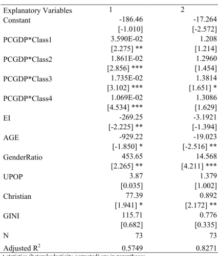
Table 1 – The Regression Equations
Explanatory Variables 1 2 Constant -186.46 -17.264 [-1.010] [-2.572] PCGDP*Class1 3.590E-02 1.208 [2.275] ** [1.214] PCGDP*Class2 1.861E-02 1.2960 [2.856] *** [1.454] PCGDP*Class3 1.735E-02 1.3814 [3.102] *** [1.651] * PCGDP*Class4 1.069E-02 1.3086 [4.534] *** [1.629] EI -269.25 -3.1921 [-2.225] ** [-1.394] AGE -929.22 -19.023 [-1.850] * [-2.516] ** GenderRatio 453.65 14.568 [2.265] ** [4.211] *** UPOP 3.87 1.379 [0.035] [1.002] Christian 77.39 0.892 [1.941] * [2.172] ** GINI 115.71 0.776 [0.682] [0.335] N 73 73 Adjusted R2 0.5749 0.8271
t-statistics (heterokedasticity corrected) are in parentheses. * ,**, ***significant at 10% ,5%; and 1% level, respectively
In Regression 2, the dependent variable and the explanatory variables related to income classes are in natural logarithmic form
Table 1 displays the OLS estimation results, which we shall now analyse, considering both regressions.
REGRESSION 1. (i) All the income class countries variables are statistically significant. The results show that an increase of 1 USD in per-capita GDP will lead to an increase of 0.036 USD in the per-capita lottery sales of a country ranked in the first class.
10 For classes 2, 3 and 4, the impacts on sales are 0.019 USD, 0,017USD and 0,011 USD, respectively. This leads us to conclude that the changes in income have a positive effect on lottery sales in all income class countries, but this effect is decreasing: the income changes have the greatest impact on per-capita sales for the income-class 1 countries and the least impact for those of class 4. As the effect is small and decreasing, we may conjecture that it would appear negative if more countries and years, another model specification or more income-class countries were applied. Garrett (2001), using a cross-sectional method and logs in variables, found a negative coefficient for the highest income-class countries (class 4).
The effect of changes in levels of education on lottery sales is negative, which is as expected. The increase of 1% in the Education Index (EI) diminishes per-capita lottery sales by approximately 270 USD. In this regression, the EI appeared significant at 5%. The higher the percentage of people aged between 15 and 29 (AGE), the fewer lottery products are sold. This variable (AGE) is significant at 10% in this model. Consistent with our expectation, the coefficient on gender ratio is positive and significant. The increase of 1% in a country’s male to female ratio implies an increase in per-capita lottery sales of almost 454 USD. The sign on the percentage of urban population is positive, which is as we expected, but it is not significant. We can conclude that Christians, on average, purchase more lottery products than the adherents of other religions (having an additional 1% of Christians in a country implies an increase of about 77 USD of per-capita lottery sales). In this regression, the variable is significant at 10%. The sign on the Gini index is positive. Countries in which inequalities are more marked will consume more lottery products. Although not significant, this relation is in harmony with our prior expectation. A 1% increase of this index implies an increase of about 116 USD in a country’s per-capita lottery sales.
REGRESSION 2. When considering the natural logarithmic of per-capita sales, the results obtained for the income classes are different from those in Regression 1. The income-class variables, except for class 3, are not significant. The results show that for the three lowest income-class countries, changes in income lead to a change in the demand for lottery products of 1.21%, 1.30% and 1.38% respectively. For the highest income-class countries, changes in income lead to an increase of 1.31% in lottery sales. The results provide evidence that income elasticity increases up to income-class 3 countries (where income has the greatest impact on lottery sales) and decreases in the fourth income-class. These results partially confirm Garrett’s (2001) findings, since our study did not find a negative coefficient for the highest income-class countries. Therefore, the results of this paper do not confirm the hypothesis that lottery products may be considered an inferior good in countries having the highest level of per-capita GDP. The results obtained for the Education index (EI), considering the logarithmic of per-capita lottery sales, show the same trend as that observed in the previous regressions. The increase of 1% in this index leads to a decrease of 3.19% in a country’s per-capita sales. In addition, the variable EI is not significant. In this regression, the conclusion on the results obtained for the variable AGE is similar to those in the preceding regression. The increase of 1% in the percentage of the population aged between 15 and 29 will imply a decrease of about 19% in a country’s per-capita sales. Although the sign remains negative, the variable shows higher significance in this regression (at 5%). The variation of gender ratio by 1% implies an increase of about 14.57% in a country’s per-capita sales.
11 This result and its significance are consistent with those obtained in the previous regression. An increase of 1% in a country’s urban population leads to a rise of per-capita lottery sales of about 1.38%. Although the sign is positive, the variable is not significant in the model. The sign of the coefficient on the Christian population remains positive in this regression.Thus, we can infer that an increase of 1% in the percentage of a country’s Christians implies an increase of 0.89% in per-capita lottery sales. While not significant, the coefficient on the Gini index shows the expected sign. The variation of the Gini index by 1% implies an increase in per-capita lottery sales of approximately 0.78%.
Implications and Conclusion
This study has fulfilled the stated objectives and the results confirm the hypothesis that lottery sales vary across income classes. Another interesting result is that in both regression equations and for all income classes, the changes in a country’s income always produce the same effect on lottery sales. So, we cannot concur with Garrett (2001, p.222) that: “lottery tickets appear to be inferior goods in countries having the highest level of per-capita GDP”. However, the regression results from equation 1 confirm the hypothesis that lotteries are regressive and states can constitute a form of exploitation by the State of the poorer sections of its population: when income increases, the low income-class countries spend more on lottery products than the higher income-class countries. These results suggest that there may be an income class cut-off point from which gambling may decrease. In other words, there may be a point at which lottery sales reach their maximum and then start to decrease. Unlike Garrett (2001), our study did not find a negative coefficient for the highest income-class countries. Hence, this paper cannot conclude that lottery products may be considered an inferior good in countries having the highest levels of per-capita GDP. In future research, it would useful to have a panel data with more countries and years and a distribution by deciles instead of quartiles in order to test this hypothesis again.
Other interesting results were obtained. Countries with higher levels of education sell fewer lottery products. From a practical point of view, it appears that the higher the level of education, the more informed a country’s population is in respect of the probabilities of winning a prize and thus, the less is the consumption of this type of product. The higher the percentage of the population segment aged between 15 and 29, the fewer lottery products are sold. The results show that countries in which the percentage of males is higher than that of females reveal higher lottery sales. Christians, on average, purchase more lottery products than the adherents of other religions. The paper did not find any statistical significance for the percentage of a country’s urban population and Gini index.
It is important to stress that this study is a cross-sectional study, in which the lack of a panel data and more qualitative information limits the conclusions and the generalisation of results. A panel data set, having both a cross-sectional and a time series dimension, allows the sample size to be increased, in addition to the use of a panel data econometric methods that are somewhat more advanced. This study has incorporated a number of factors that affect lottery ticket-buying behaviour. However, numerous issues remain beyond the scope of the present study, yet still merit investigation. For example, this paper does not consider the presence of substitute gambling products and does not
12 control for the effects of price changes in these differentiated goods, ceteris paribus, on the demand for lottery products. If we introduce a new parameter to be estimated - the elasticity of substitution between lottery products and other gambling products - the elasticity of demand for lottery will be affected. However, as the market is characterised by product differentiation, we believe that the main conclusions of this paper remain valid.
The scope of our study relied on a static analysis. An historical dimension would be of great interest, in order to analyse whether the factors and behavioural characteristics identified are maintained through time. In the present study, socio-economic variables – income, education, age, gender, religious background – provided a useful model to understand the determinants of lottery sales. Nonetheless, there are other explanatory variables, particularly qualitative variables, and other econometric specifications that may be considered. Some empirical studies have used surveys to discover the characteristics behind lottery gambling. Such surveys could reveal other features and would be of value in guiding the selection of the explanatory variables in the econometric studies, as well as complementing the quantitative studies.
References
Abbott, M., Volberg, R., Bellringer, M. and Reith, G. 2004. ´A review of research on aspects of problem gambling´. Gambling Research Centre. Auckland University of Technology.( available on:
http://www.rigt.org.uk/documents/a_review_of_research_on_aspects_of_problem_gam bling_auckland_report_2004.pdf)
Abbott, M.A. and Clarke, D. 2007.´Prospective problem gambling research: Contribution and potential´, International Gambling Studies, 7(1), pp.123-144.
Balabanis, G. 2002. ´The relationship between lottery ticket and scratch-card buying behavior, personality and other compulsive Behaviors´, Journal of Consumer Behaviour, 2(1), pp. 7-22.
Blalock, G., Just, D.R. and Simon, D.H. 2007. ´Hitting the Jackpot or Hitting the Skids: Entertainment, Poverty, and the Demand for State Lotteries´, American Journal of Economics and Sociology, 66 (3), pp. 545-570.
Binde, P. 2007. ´Gambling and religion: Histories of concord and conflict`, Journal of Gambling Issues, 20, pp. 145-165.
Chalmers, H. and Willoughby, T. 2006. ´Do predictions of gambling involvement differ across male and female adolescents?’, Journal of Gambling Studies, 22, pp.373-392. Clotfelter, C. T. and Cook, P.J. 1989. ´The demand for lottery products´, NBER Working
Paper 2928.
Clotfelter, C., Cook P. J., Edell J. A., and Moore, M. 1999. ´State Lotteries at the Turn of the Century: Report to the National Gambling Impact Study Commission´. Duke University. (available on:http://govinfo.library.unt.edu/ngisc/reports/lotfinal.pdf)
Croups, E., Haddock, G. and Webley, P. 1998. ´Correlates and predictors of lottery play in the United Kingdom’, Journal of Gambling Studies, 14(3), pp. 285-303.
Diaz, J. 2000.´Religion and gambling in sin-city: A statistical analysis of the relationship between religion and gambling patterns in Las Vegas residents´, The Social Science Journal, 37 (3), pp.453-458.
13 Friedman, M. and Savage, L.J. 1948. ´The utility analysis of choices involving risk´,
Journal of Political Economy, 56(4), pp. 279–304.
Ghent, L. S. and Grant, A.P. 2006. ´Are voting and buying behavior consistent? An examination of the South Carolina education lottery´, Public Finance Review, forthcoming(available on http://www.ux1.eiu.edu/~cflsg/sclottery.pdf).
Garrett, T. A. 2001. ´An international comparison and analysis of lotteries and the distribution of lottery expenditures´, International Review of Applied Economics, 15(2), pp. 213-227.
Giacopassi, D., Nichols, M.W. and Stitt, B.G. 2006. ´Voting for a lottery´, Public Finance Review, 34(1), pp. 80-100.
Lam, D. 2006. ´The influence of religiosity on gambling participation´, Journal of Gambling Studies, 22, pp.305-320.
Layton, A. and Worthington, A. 1999. ´The impact of socio-economic factors on gambling expenditure´, International Journal of Social Economics, 26 (1/2/3), pp. 430-440.
Kallick, M., Suits, D., Dielman, T., and Hybels, J. 1979. ´A survey of American gambling attitudes and behavior´, Ann Arbor, MI: Institute for Social Research, University of Michigan.
Kearney, M.S. 2005. ´State Lotteries and Consumer Behavior´, Journal of Public Economics, 89, pp. 2269-2299 .
Miyazaki, A. D., Langerderfer, J. and Sprott, D.E. 1999. ´Government-sponsored lotteries: Exploring purchase and nonpurchase motivations´, Psychology & Marketing, 16(1), pp. 1-20.
Miyazaki, A. D., Brumbaugh, A.M. and Sprott, D.E. 2001. ´Promoting and countering consumer misconceptions of random events: The case of perceived control and state-sponsored lotteries´, Journal of Public Policy & Marketin, 20(2), pp. 254-267.
Shiller, R. J. 2000. Irrational Exuberance, Princeton University Press, Princeton.
Sproston, K. 2002. Partipation and Expenditure in the National Lottery. Report Prepared for National Lottery Commission.
(available
on:http://www.nationallotterycommission.gov.uk/UploadDocs/Contents/Documents/Pa rticipation and expenditure report 2002.pdf)
Welte, J.W., Barnes, G., Wieczorek, W., Tidwell, M. and Hoffman, J. 2007.´Type of gambling and availability as risk factors for problem gambling: A Tobit regression analysis by age and gender´, International Gambling Studies, 7(2), pp.183-198.
Internet references http://www.camelotgroup.co.uk/index.html http://www.devdata.worldbank.org http://www.census.gov/ipc/www/idb http://hdr.undp.org/en/ https://www.cia.gov/library/publications/the-world-factbook/fields/2122.html
14
Apendix 1:
Table 2 – The Regression Equations with 4 Age Groups
Explanatory Variables 1 2 Constant -27,14 -17,51 (-0,0556) (-2,6269) PCGDP*Class1 2,69E-02 1,19 (1,9642)* (1,2456) PCGDP*Class2 1,47E-02 1,27 (2,6098)** (1,4750) PCGDP*Class3 1,60E-02 1,37 (3,7821)*** (1,6988)* PCGDP*Class4 9,87E-03 1,30 (5,1650)*** (1,6875)* EI -281,37 -3,73 (-1,5665) (-1,6657) AGE1 -974,18 -16,69 (-1,2138) (-1,4602) AGE2 2016,28 10,40 (1,4980) (1,2143) AGE3 -1518,61 -5,63 (-2,1130)** (-0,9184) AGE4 618,15 3,98 (0,4875) (0,5112) GenderRatio 212,77 13,53 (0,4775) (4,0505)*** UPOP -23,78 1,16 (-0,2487) (0,8801) Christian 109,83 1,07 (3,6219)*** (2,4701)** GINI -54,88 0,32 (-0,3371) (0,1256) N 73 73 Adjusted R2 0,6260 0,8248
t-statistics (heterokedasticity corrected) are in parentheses. * ,**, ***significant at 10% ,5%; and 1% level, respectively
In Regression 2, the dependent variable and the explanatory variables related to income classes are in natural logarithmic form.
15
Appendix 2: List of countries distributed into 4 quartiles basing on per capita GDP
Total 2004 Per-Capita Sales (in USD)
2004 Per-Capita GDP in PPP (in USD) Quartile 1 Ghana 2,59 224 Ethiopia 0,20 756 Niger 2,05 779 Madagascar 0,16 857 Congo 0,57 978 Mali 0,03 998 Benin 1,42 1.091 Kenya 0,44 1.140 Burkina Faso 3,17 1.169 Mozambique 0,19 1.237 Togo 4,57 1.536 Ivory Coast 6,74 1.551 Senegal 5,36 1.713 Moldova 0,28 1.729 Gambia 1,40 1.991 Zimbabwe 0,12 2.065 Bolivia 0,31 2.720 India 2,95 3.139 Morocco 7,08 4.309 Philippines 3,17 4.614 Quartile 2 Peru 2,13 5.678 Lebanon 28,27 5.837 China 4,55 5.896 Ukraine 0,44 6.394 Algeria 0,55 6.603 Macedonia 6,94 6.610 Panama 160,56 7.278 Kazakhstan 1,21 7.440 Turkey 17,27 7.753 Bulgaria 18,44 8.078 Thailand 40,09 8.090 Brazil 5,45 8.195 Romania 11,56 8.480 Uruguay 21,34 9.421 Costa Rica 47,72 9.481 Mexico 11,57 9.803 Malaysia 87,57 10.276 Chile 18,81 10.874 South Africa 24,73 11.192 Latvia 3,57 11.653
16 Total 2004 Per-Capita Sales (in USD) 2004 Per-Capita GDP in PPP (in USD)
Quartile 3 Mauritius 16,66 12.027 Trinidad 160,91 12.182 Croatia 29,80 12.191 Poland 26,99 12.974 Lithuania 12,38 13.107 Argentina 57,82 13.298 Estonia 12,42 14.555 Slovakia 22,57 14.623 Hungary 72,81 16.814 Malta 219,35 18.879 Czech Rep. 33,99 19.408 Portugal 157,71 19.629
Korea, R(South Korea) 86,33 20.499
Slovenia 19,43 20.939 Greece 528,46 22.205 Cyprus 346,32 22.805 New Zealand 136,03 23.413 Israel 200,07 24.382 Spain 450,16 25.047 Singapore 826,11 28.077 Quartile 4 Italy 407,28 28.180 Germany 189,77 28.303 Japan 94,52 29.251 France 236,86 29.300 Sweden 284,51 29.541 Finland 399,92 29.951 Australia 193,02 30.331 U.K. 184,56 30.821 Hong Kong 138,86 30.822 Belgium 257,46 31.096 Canada 205,76 31.263 Netherlands 97,44 31.789 Denmark 327,82 31.914 Austria 308,57 32.276 Switzerland 225,81 33.040 Iceland 210,13 33.051 Norway 432,64 38.454 Ireland 255,26 38.827 United States 204,33 39.676 Luxembourg 185,25 69.961