Customization of a software of finite elements to
analysis of concrete structures: long-term effects
Customização de um programa de elementos finitos
para análise de estruturas de concreto: efeitos de
longa duração
a Federal University of Rio Grande do Sul, Post-Graduation Program in Civil Engineering, School of Engineering, Porto Alegre, RS, Brazil.
Received: 23 Aug 2017 • Accepted: 25 Jan 2018 • Available Online:
F. P. M. QUEVEDO a
R. J. SCHMITZ a
I. B. MORSCH a
A. CAMPOS FILHO a
D. BERNAUD a
Abstract
Resumo
Concrete is a material that presents time-delayed effects associated with creep and shrinkage phenomena. The numerical modeling of the creep is not trivial because it depends on the age of the concrete at the time of loading, which makes necessary to store the history of loads to apply the principle of superposition. However, a problem formulated in finite elements has many points of integration, making this storage impossible. The Theory of Solidification, together with incremental algorithm developed by Bazant e Prasannan ([1], [2]), solves this problem. Therefore, this paper presents the adaptation of this algorithm to a finite element commercial software (ANSYS) considering the creep, according to the CEB-FIP Model Code 1990 [3]. The results demonstrate that the deformations provided by this adaptation are in accordance with the analytical solution given by the CEB-FIP MC90, including cases where the loads are applied at different ages of the concrete.
Keywords: concrete long-term effects, creep and shrinkage on concrete, finite element method.
O concreto é um material que apresenta efeitos diferidos no tempo, que estão associados aos fenômenos de fluência e retração. A modelagem numérica da fluência não é trivial, pois depende da idade do concreto no instante de aplicação do carregamento, o que torna necessário arma
-zenar a história de carga para posterior aplicação do princípio da superposição dos efeitos. Contudo, um problema formulado em elementos finitos possui muitos pontos de integração, tornando esse armazenamento impossível. A Teoria da Solidificação, juntamente com o algoritmo incremental desenvolvido por Bazant e Prasannan ([1], [2]), permitem resolver esse problema. Esse artigo apresenta a adaptação desse algo
-ritmo em um programa de elementos finitos (ANSYS), considerando a fluência conforme formulado pelo Código Modelo CEB-FIP 1990 [3]. Os resultados comprovam que as deformações previstas por esta adaptação estão em conformidade com a solução analítica dada pelo CEB-FIP MC90, incluindo situações em que as cargas são aplicadas ao longo de diferentes idades do concreto.
1. Introduction
Since it was discovered by Hatt [4] in 1907, several materials re
-searchers have been studying long-term effects of concrete. Cur
-rently, this behavior is separated in creep and shrinkage, and the main difference between them is that the first one depends on the loading, while the second does not.
Creep is characterized by continuous and gradual advancement of deformations under constant stress. This deformation (excluding the
Poisson effect) has the same direction of the loading and is divided, for analytical convenience, into basic and drying creep. The first oc
-curs without water exchange with the environment and can be mea
-sured when the specimen is immersed in a 100% humidity ambience. On the other hand, the second is when water exchanged occurs with
the environment and therefore depends on the relative humidity of the air and the exposure of the specimen to the ambience.
The shrinkage is the reduction of the volume due to the gradual loss of water independent of the tension. It is also divided, for conve
-nience, into autogenous and drying shrinkage. The first occurs with
-out loss of water to the environment and is a consequence of the re
-moval of water from the capillary pores by the hydration reactions of the cement, while the second one, also called hydraulic shrinkage, occurs due to the loss of water to the environment. As the shrinkage is associated with the volume reduction, this phenomenon induces internal tensile stresses that can cause fissures on the concrete. In this aspect, the minimization of shrinkage is one of the main reasons for the concrete curing procedure, which seeks to reduce water loss
in the early ages as the concrete is just developing its resistance.
These deformations of the concrete have important influence on
the structural behavior, since these deformations can reach 2 to 3 times the value of the instantaneous deformation, according to
RILEM Technical Committees [5]. Several semi-empirical formula
-tions for predicting creep and shrinkage strain are available in the literature and in design standards. However, these formulations, in general, present a certain approximation when compared to ex
-perimental tests. As noted by Fanourakis e Ballim [6], the error can range from 25.9% until 67.4%, depending on the formulation and
test used in the comparison.
This paper is based on the works of Dias [7], Dias et al. [8], Que
-vedo [9] and Schmitz [10], who used the long-term concrete for
-mulation proposed by the Comité Euro-International du Béton (CEB-FIP MC90) [3] adapted to the Solidification theory of the Ba
-zant and Prasannan ([1], [2]) for their studies involving composite
beams, tunnels and bridges, respectively. The creep formulation
of the CEB-FIP MC90 has the advantage of fitting perfectly with the Bazant and Prasannan theory. This is possible because this formulation separates the coefficient of creep in a factor that de -pends on the age of the concrete and another one that de-pends exclusively on the age of the load. Such separation does not occur
in current formulations, for example, in the Féderation Internatio
-nale du Béton [11]. In view of this decomposition, the incremental algorithm developed by Bazant and Prasannan [2] allows to model efficiently the cases in which there are histories of variable loads (or stresses). The use of the CEB-FIP MC90 formulation without
this algorithm, in a non-linear analysis, requires that all increase and decrease of stresses need stored to apply the superposition
principle. This procedure would make it impossible to analyze in situations with many finite elements.
Therefore, this paper will present this adaptation with some com
-ments on the customization and use of this model in ANSYS. At the
end, some results are presented to validate this approach.
2. Numerical model
In this item, the model for the concrete is presented considering the long-term behavior, especially the creep and the adaptation of
the CEB-FIP MC90 expressions to the Solidification theory.
2.1 Adaptation of the CEB-FIP MC90 creep
formulation to the Solidification theory
Considering that the concrete is an aging material and creep is the portion of the long-term behavior directly related to the loads applied to the structure, the age of the concrete at the times of
application of the loads directly influences the creep deformations. The theory of Solidification proposed by Bazant and Prasannan
Figure 1
([1], [2]) aims to facilitate the numerical solution of this particularity between creep and the age of loading. These authors proposed a
model that considers aging as an isolated factor, associated only
to the volume of solidified concrete, overtime.
Figure 1 shows in a schematic form the model proposed by Bazant and Prasannan for the concrete behavior. The total deformation is
given by the sum of four parts: elastic, viscoelastic, viscous and a part that is independent of the stress, corresponding to the
defor-mations by shrinkage, thermal and cracking. The creep strain is divided into two parts: one called “viscoelastic” and another called “viscous”. This division intends to treat the shape of the curve creep in relation to the loading age. For small loading ages, the function takes the form of power (primary creep), and for larger loading ages, the curve takes the predominantly logarithmic form (which is often conveniently represented as a straight line on the semi-log scale of time) (Bazant e Prasannan, [1]).
As shows in Figure 1, the viscoelastic portion εv is associated to
the volume fraction of concrete already solidified v(t) and with a
loading age depending of the creep coefficient Ф(t – t0), where time t is the current age of the concrete and t0 is the age at which the
load was applied. Similarly, the viscous portion εf depends on the
hydrated cement fraction h(t) and the coefficient ψ(t – t0)
depen-dent on the loading age (Bazant e Prasannan, [1]). In Figure 1, the
factor Ф(t – t0) is represented by a Kelvin-Generalized
rheologi-cal model (or also known as the Kelvin chain). Since this function
depends only on the age of the load, the parameters of the Kelvin chain become constant, facilitating the development of the incre-mental algorithm described later.
From these considerations the creep function J(t, t0), according to
the theory of Solidification is given by expression (1):
(1)
Where E0 is the modulus of elasticity for the aggregates and
mi-croscopic particles of the cement paste, γ(t – t0) is the microvisco-elastic deformation, and η(t) is the apparent macroscopic viscosity
dependent on the age of the concrete. In the CEB-FIP MC90 [3]
the creep function is given by (2):
(2)
Where Ec (t0) is the tangent modulus of elasticity at t0, Eci is the
tan-gent modulus of elasticity at 28 days and Ф(t, t0) is the creep
coef-ficient. In [3] the coefficient of creep is divided into two factors: ϕ0
which is related to the age of load application and βc (t – t0) which
describes the shape of the creep curve with the age of the load. Comparing (1) and (2) we have expressions (3), (4), (5) and (6) to
adapt both formulations.
(3)
(4)
(5)
(6)
Equality (6) occurs because Bazant and Prasannan ([1], [2]) treat
the creep curve separating it into two parts: one corresponding to the first ages (viscoelastic) and another referring to posterior ages (viscous). However, the CEB-FIP MC90 formulation does not make
this distinction by representing the behavior of the creep curve only by the function βc (t – t0).
Although the Bazant and Prasannan Solidification theory ([1], [2]) consider a factor to the stress level F[σ(t)], the model presented in CEB-FIP MC90 does not consider this behavior and, therefore, this factor does not appear in this adaptation. However, due to this simplification, the stress limit of 40% of the average compressive strength is imposed. This limit is fundamental to keep the concrete in viscoelastic regime, where the principle of superposition of the effects is valid. Therefore, during the numerical analysis, consid -ering this adaptation, one must respect this limit in order do not underestimate the deformations.
2.2 Curve fitting to the coefficient of creep factor
that is independent of the concrete age
As previously mentioned a Kelvin chain represents the coefficient
of creep that is independent of the concrete age in the incremental
algorithm of Bazant and Prasannan [1]. Since this factor is inde -pendent of the concrete age t0, the parameters of this chain
(modu-lus of elasticity of the springs and coefficient of viscosity of the
dashpots) also become constant and this facilitates the deduction
of the incremental algorithm, which uses a numerical solution for
the integral of the strain rate.
The equations that represent the behavior of the Kelvin chain are
presented in expressions (7). Due to the serial configuration of the
μ-th units of Kelvin, for each unit, the applied tension σμ is the same as the total σ and the total strain of the chain γ is given by the sum of the deformation of the units.
(7)
Where Eμ is the modulus of elasticity, ημ is the viscosity and γμ is the
deformation of μ-th unit of the chain. Solving the differential equa
-tion presented in (7) we get the expression (8) which is known as the Dirichlet (or Prony) series. The term τμ is called the retardation
time of the μ-th unit of the chain.
(8)
In order to use the Solidification theory, adapted to CEB-FIP MC90,
the expression (8) must represent the function βc (t – t0), as shown in (4). This can be done by discretizing this function into L points
and fitting it to (8) through the least squares method. According to Dias [7] this can be done by assembling and solving the system [A]{X}=[B], whose elements are given by (9), (10) and (11).
(9)
(10)
(11)
ob-tained. It is important to emphasize that the fitting of the model can
lead to negative values of modulus of elasticity in certain elements,
which do not have physical correspondence with the mechanical
model, because it is only a mathematical adjustment. In addition, the resolution of this linear system requires the choice of the retar-dation times of the elements of the chain τμ. In order for the matrix
[A] to be well conditioned, Bazant and Prasannan [2] propose that
the retardation times are chosen as a logarithmic increase of base 10 according to (12).
(12)
According to Dias [7], the retardation times should cover half the
analysis period tmax and τ1 be small enough to represent the behav-ior of the creep curve at early ages, as expressed in (13).
(13)
According to Dias [7], the quantity N of Kelvin units was deter -mined to be the maximum possible until one has τμ greater than or equal to τN. However, no more than six Kelvin units.
In addition to the retardation times, for the system solution, it is also necessary to choose the L points of the function βc (t – t0) for the adjustment. Since this function is related to the age of the load,
in fact, the question is to define the age intervals (tk – t0), where t0
is the age of the concrete at the time of the first load application and k=1,…,L are the points. Considering that the behavior of the function is more pronounced in the first loading ages, an effective choice is to keep the time intervals constant in a logarithmic scale.
Thus, the points for adjustment can be obtained through the
recur-rence formula (14) (Bazant e Prasannan [1], [2]).
(14)
So in that, the parameter m is the number of steps per decade,
according to [7], and around 10 for a good precision. In addition, the first time interval chosen corresponds to one tenth of the first loading age of the structure [7], according to expression (15).
(15)
And the number of points L can be determined to be that
neces-sary to cover study time, in other words, until t(k+1) – t0 is greater than tmax – t0.
2.3 Incremental algorithm
Then, the adjusted parameters (Eμ, τμ) of the Kelvin chain can be
used in the incremental algorithm. Expressing the total deforma
-tion in terms of rates, we have (16).
(16)
Where is the elastic deformation rate,
is the viscous strain rate and is the sum of all
strain rates independent of stress (shrinkage, thermal and cracking).
Integrating expression (16) through the trapezoid rule, for an inte-gration interval from ti to t(i+1) we obtain (17), where E(i+1/2) e v
(i+1/2)
are the values corresponding to the middle of the interval between
ti and t(i+1).
(17)
If the increment of elastic deformation is separated from the
remain-der of the deformation, we can write (18), the part ∆ε* being all
defor-mation which is non-elastic (creep, shrinkage, thermal and cracking) and E* the equivalent modulus of elasticity, both to be deducted.
(18)
The creep strain is obtained by assuming that the stress varies
linearly between two consecutive time steps, according (19). This assumption, as will be seen later, imposes the need for a small
increment of time.
(19)
By introducing (19) into (7), we have (20).
(20)
Since is the strain of the μ-th Kelvin unit in the next time step
(i + 1) and is the μ-th Kelvin unit strain for the current time step i.
In the same way σi is the current stress and ∆σ is the stress
incre-ment considering the time interval between ti and ti+1. This increase of
deformations can be calculated as , resulting in (21).
(21)
The first factor of the first term to the right side of the equality in
(21) is the viscous deformation of the μ-th Kelvin unit of step i, expressed by (22).
(22)
In the same way as expression (22), in (23) we have the viscous deformation of the Kelvin unit of the next step i +1.
(23)
As deduced by Dias [7], by substituting given by equation
(20), in the expression (23) results the expression (24), which is
still ignoring the viscous deformation aging. The aging is
consid-ered including the volume of solidified concrete in expression (24),
so that the viscous deformation is given by equation (25).
(24)
(25)
For the increment of viscous deformation, first replace the expres -sion (21) in (17) having the increment of total strain, given by the expression (26).
(26)
Considering the separation of the elastic deformation part
pro-posed by equation (18) we can define the expression for ∆ε* and E*, which are according to equations (27) and (28).
(28)
Generalizing the expressions for a three-dimensional domain,
con-sidering an isotropic material, we have (27) that become a matrix
equation, according (29).
(29)
Where is calculated by the expression (30), generalized of the
(25), considering which [Dμ]-1 is the inverse of the linear isotropic
constitutive matrix, and the elastic modulus is equal to .
(30)
In expression (30), it can be verified that it is necessary to store
only the viscous deformation corresponding to the previous step , avoiding to store all the loading history.
During the iterative solution process, in addition to determining
the increment of non-elastic deformation, it is also necessary to update the constitutive matrix and correct the increment of total deformation in the calculation of the stress increase. Generalizing to a three-dimensional domain the expression (18) and isolating the stress increment is obtained (31).
(31)
Where [D*] is a linear isotropic constitutive matrix considering the modulus of elasticity E* calculated by the expression (28) and Poisson’s ratio of the concrete.
3. ANSYS customization
3.1 Operation of programmable tool UserMat
ANSYS offers a series of programmable features (User Program
-mable Features – UPF) that allows the user customize models as
-pects through subroutines wrote in Fortran77. Once the change is
made, the subroutines are compiled and associated to the main
program ANSYS. One of these subroutines, the UserMat, is specific to customize the material laws; therefore, it is ideal to insert the
concrete model.
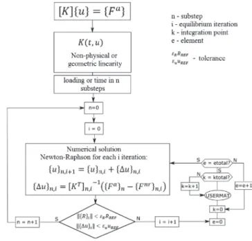
The iterative process used by ANSYS to solve nonlinear problems consists to apply the Newton-Raphson procedure. For each time/
load increment n (also called substep) it is calculated i equilibrium
iterations until the convergence criterion is satisfied. The expres
-sions (32), (33) and the Figure 2 (adapted of ANSYS [13]) explain
this process.
(32)
(33)
Where {u}n,i+1 is the actualized nodes displacement vector of the
substep n, {u}n,i is the nodes displacement vector of the iteration i,
{∆u}n,i is the nodes displacement increment vector of the
itera-tion i, [KT]
n,i is the tangent stiffness matrix (or Jacobian matrix
of Newton-Raphson method), {Fa}
n+1 is the applied forces vector,
{Fnr}
n,i is the internal forces vector of the iteration i, {R}n,i is the
unbalance vector or residual of the iteration i used in the
conver-gence criterion. Using the nodes displacement, in each equilib -rium iteration i, it is obtained the deformations and stress in each integration point through the relations displacement-strain and
stress-strain formulated by shape functions of the Finite Element
Figure 2
Illustration of Newton-Raphson Method with
equilibrium iterations i for each substep n (ANSYS, [13])
Figure 3
Method. Therefore, for each integration point, the main program gives to UserMat the total stress, total deformations and incre
-ment of total deformations (resultants of the Newton-Raphson
iterative process) in the current time increment. The instructions programmed inside of the subroutines are responsible to collect
the material constants (defined by the user), to update the stress and the Jacobian matrix used in the iterative process. The Figure 3 shows a flow chart that summarize the UserMat operation in -side the nonlinear analysis.
3.2 Implementation of viscoelastic model in UserMat
ANSYS provides one UserMat with a bilinear isotropic relation of
stress-strain with the von Mises plasticity criterion. The user needs
understand this subroutine and modify according the necessity. It is important to understand all input and output arguments of the subroutine for creating and using the less number of variables that is possible in the material behavior customization. Special atten-tion should be given to UserMat input and output variables, since
they must not be deleted. However, the local variables, which in the most part are referenced to the von Mises plastic behavior, can be excluded without compromise the subroutine operation.
The UserMat consists of four internal subroutines depending on the strain components number (or stress) and of the dimensions involved
in the problem (1D, 2D, 3D). In the present paper was customized the
more generic subroutine of the four, the UserMat3D, that corresponds
to problems with more than 3 components, as three-dimensional
problems (6 components, 3 directions), plane strain and axisymmetric
(both with 4 stress components and 2 directions).
The user is free to create how many local variables are necessary. However, local variables lose their value when the subroutine fin
-ish during the equilibrium iterations. When it is necessary holding
the value of some variables between the substeps it is necessary
to store in array of state variables ustatev (Figure 4–(d)). This array can be used directly without creating a variable. However, in order
that the ustatev arrayis dimensioned it is necessary to declare its
size in the script through the command TB, STATE during the ma
-terial assignment (Figure 4–(a)). It is not recommended save the variables values in a COMMON instruction, except the ones that
maintain constant values during the analysis. This type of
declara-tion brings problems in the ANSYS parallelizadeclara-tion, because many parallel processes can access and overwrite this memory space si -multaneously. It is also possible to visualize the ustatev array values
in the post processor through the command PLSOL,SVAR, [vari
-able position in the array], provided that they are saved through the command OUTRES,SVAR,ALL.
The input data array prop contain the material constants that
are completed through the script during the material definitions. This array is dimensioned through the command TB, USER (that define the quantity nprop of proprieties) and the proprieties
values are attributed through the command TB,DATA (Figure 4-(a), Figure 4-(c)).
Other important aspect about the use of UserMat in concrete
vis-coelasticity is the definition of times and concrete ages during the analysis. The ANSYS provides the variable time and dtime that are
shared between script and the UserMat and represent the analysis
current time and the time increment, respectively (Figure 4-(b)). In general way the customized UserMat3D follows the steps:
1) calculation of the non-elastic strain increment {∆ε*};
2) calculation of the elastic strain increment: {∆εe} = {∆ε} - {∆ε*},
where {∆ε} is the total strain increment informed by ANSYS (comes from the Newton-Raphson iterative process);
Figure 4
APDL commands for (a) material definition, (b) definition of time and analysis time increment.
Whitin the
Usermat3D
: (c) assignment of the variables related to the material and (d) storing principal
3) calculation of the constitutive matrix [D];
4) calculation of the stress increment {∆σ} = [D] {∆εe};
5) update of the Jacobian matrix (∂∆σij) ⁄ (∂εij) = [D];
6) calculation of the update stress {σ(i+1)} = {σi} + {∆σ}.
When it is decreased the non-elastic strain increment of the total
strain increment (step 2), the Newton-Raphson procedure will
compensate this increasing the total strain increment during the
equilibrium iterations until the convergence will be satisfacted. In this way it is introduced the concrete viscous deformation in
the problem.
In the customized UserMat, the concrete is defined with an initial
instant ti, option that can be useful when it is used the birth/death recurs of the elements to simulate the construction procedure of a bridge or a tunnel, for example. The material age is given by tmat = time - ti. However, the phenomena of shrinkage and creep
depend of, respectively, the age of the beginning of shrinkage ts
and the time when the load is applied t0. In this way, the phenom
-enon of shrinkage starts when time > ti, that is at the moment of the
concrete birth, but considering ts, according to the CEB-FIP MC90
expressions. The creep phenomenon starts when time > t0, that is
at the moment that the piece gets loaded, where the load age is
equal to tmat - t0.
In Quevedo [9], there is the customized UserMat subroutine for the
viscoelastic concrete, with creep and shrinkage phenomena) and there are instructions to add it in the ANSYS main program.
3.3 Compatible finite elements
The UserMat3D can be used in three-dimensional generic
prob-lems, plain strain or axisymmetric. For the first case can be used
the elements SOLID185 and SOLID186, for the others two situ
-ations there are the elements PLANE182 and PLANE183. The elements PLANE182 and PLANE183, presented in Figure 5, are elements quite similar, both are quadrilaterals and they have with two degrees of freedom at each node (translations in the two plane direc
-tions where are inserted). The main difference between them is that the PLANE182 has four nodes and, therefore, linear shape functions while the PLANE183 has eight nodes and, therefore, quadratic shape
functions. Besides the quadrilateral shape, both encompass the
trian-gular shape, being this shape not advisable for PLANE182 because it
presents little precision on the interpolation.
The elements SOLID185 and SOLID186, illustrated in Figure 6, are solid elements; therefore, their nodes have three degrees
of freedom of displacements in the directions x, y e z. So again
the main difference between the two elements is the shape
Figure 5
Plane elements: (a) PLANE182 and (b) PLANE183
(ANSYS, [14])
Figure 6
functions degree, the SOLID185 has eight nodes and, therefore, linear shape functions while the SOLID186 has twenty nodes and,
therefore, quadratic shape functions. Both elements encompass also the tetrahedral and pyramidal shape.
The choice of quadratic elements should consider the number of
elements in the mesh. Due to a nonlinear analysis, where the sys -tem of equations is solved at each increment of time, the process-ing time may be large.
For reinforced concrete analysis, both classes of elements (PLANE and SOLID) have the incorporated reinforcement feature through the inclusion of the elements REINF263 (for plane elements) and REINF264 (for solid elements) after setting of the concrete mesh
elements. These elements are ideals to represent reinforcement,
because they have only axial stiffness and they can be inserted
in any position and direction inside the concrete elements. This
aspect brings a large advantage in comparison with the ANSYS concrete element (SOLID65) that the reinforcement is not incorpo
-rated and it needs a much more refined mesh.
4. Validation and numerical examples
In order to validate the programmed model in UserMat, it was done
some numerical simulations, being that the first two tests served to compare the results with the analytical solution obtained with
CEB-FIP MC90 formulations. These tests consisted in modeling the compression experiment, as in Figure 7. The proprieties con -sidered in these initial simulations are presented in Table 1. The
first test consisted to apply compression stress increments equal to 5 MPa at 10, 50 and 75 days, being the analysis made until 100 days. The second test consisted to apply 5 MPa constant until 100 days. The Figures 8 and 9 present the obtained results decom
-posed in total strain, elastic, creep and shrinkage. On the two tests, it was verified perfect agreement with the numerical simulations
Figure 7
Model to verify the implementation of the
viscoelastic model
Table 1
Concrete parameters in the initial tests
Parameter Symbol Unit Value
Characteristic compressive strength fck MPa 40
Coefficient which depends on concrete type s adm 0.25
Poisson’s ratio ν adm 0.2
Relative humidity of ambient environmental RH % 70
Fictitious thickness hf cm 54.54
Age at the beginning of shrinkage ts days 7
Coefficient which depends on concrete type – shrinkage βsc adm 5
Temperature temp °C 20
Coefficient which depends on concrete type α adm 1
Figure 8
Test 1 with cube subjected to variable stress using
the element SOLID185
Figure 9
and analytical calculation. These tests were also repeated consid -ering one element and various elements.
The next test consisted in check the increment time influence used in the analysis. Until now, the time increment considered was only 1 day. However, the incremental algorithm of Solidification theory
suppose a stress linear variation between two consecutive time intervals. However, in fact, this variation is not linear, and this way, how bigger the time increment and the time of whole analysis, big
-ger will be the error in the creep deformation calculation. In Figure
10 are presented the results of this analysis considering only the elastic strain added the creep strain for 5 time increments: 1, 2, 5,
10 and 20 days. It can be observed that with the increment of 5 days, the error is little, around 2.5%. However, for the increment of 10 days, the error reach 4.8% and for the 20 days, it is 7.5%.
Therefore, to have better precision on the results it is suggested to use time increments minors than 5 days.
In order to compare the results with experimental data, it was
numerically simulated 5 experimental tests presented by Ross
[12]. These experimental tests consist in two cylindrical proof bodies, with diameter equal to 117.5mm and 305mm of height.
One of them subjected to load history (Table 2) and the other
without loads, to measure the deformation generated by shrink -age, and after to decrease it of the results of proof bodies
sub-jected to load, having in this way only the elastic response with creep. The concrete proprieties in the Ross’ experiments are in Table 3. To the numerical simulations, it was tested the two
Figure 10
Influence of time increment
Table 2
Stress history in Ross’ tests [12]
Tests t0 t1 t2 t3 t4 t5 tf
1 Age (days) 14 60 – – – – 140
Stress (MPa) 1.503 0 – – – – 0
2 Age (days) 28 60 91 120 154 – 190
Stress (MPa) 1.503 1.127 0.751 0.376 0 – 0
3 Age (days) 8 14 28 63 90 120 180
Stress (MPa) 1.379 1.103 0.827 0.551 0.275 0 0
4 Age (days) 8 16 28 63 90 120 180
Stress (MPa) 2.75 0.551 0.827 1.103 1.379 0 0
5 Age (days) 8 14 28 63 90 120 180
Stress (MPa) 1.379 0.827 0.275 0.827 1.379 0 0
Table 3
Concrete parameters in Ross’ tests [12]
Parameter Symbol Unit Value
Characteristic compressive strength fck MPa 38
Coefficient which depends on concrete type s adm 0.2
Poisson’s Ratio ν adm 0.15
Relative humidity of ambient environmental RH % 93
Fictitious thickness hf cm 3.939
Age at the beginning of shrinkage ts days 7
Coefficient which depends on concrete type - shrinkage βsc adm 8
Temperature temp °C 17
elements, SOLID185 and PLANE182 in axial compression, like in Figure 7. The obtained results are in Figure 11 until Figure 15. It can be observed the perfect agreement between the model with SOLID185 and the CEB-FIP MC90 formulation, being that the two curves are overlapping. About the PLANE182, it realized
that in all situations there is a little error. This error is attributed to the fact that tests are not in a plain strain or axisymmetric
conditions, that are the scope of the element. Despite this, it can
be confirmed that the UserMat3D is not restrict only to three-dimensional problems.
In addition, the difference between the experimental results and the analytical curves is because of the approximation of the CEB-FIB MC90 formulation. This variation is expected, since the for -mulation is based on a series of experiments and considerations,
including statistic, of many studies. These differences are common and inherent to the used formulation, conform it was verified by [6].
5. Conclusions
This paper proposes to present the implementation of the concrete
long-term behavior, considering the effects of creep and shrinkage, especially the creep, through the Bazant and Prasannan ([1], [2]) Solidification theory adapted with CEB-MC90 [3] expressions. The adaptation was based on Dias [7], however it was programmed in the customization feature of ANSYS. The behavior was tested and validated with analytical solution of CEB-FIP MC90 and with some experimental tests performed by Ross [12]. It was obtained an ex
-cellent agreement between the numerical and analytical results, being the difference in relation to the experimental results inherent to the CEB-FIP MC90 model.
It was verified the importance of using small time increments (minors
than 5 days) during the analysis to obtain precision in the prediction
Figure 11
Comparison with experimental test 1
Figure 12
Comparison with experimental test 2
Figure 13
Comparison with experimental test 3
Figure 14
Comparison with experimental test 4
Figure 15
of deformations. This is due to the simplification of the linear varia -tion of the stresses in the integra-tion of the strain rates adopted
dur-ing the deduction of the Solidification theory incremental algorithm. In these numerical simulations, plane (PLANE182 and PLANE183) and three-dimensional (SOLID185 and SOLID186) elements were tested in unconfined compression with one and several elements. It shows that it is possible to use this customization for three-di -mensional, plane strain and axisymmetric conditions that involve
long-term deformations concrete. In this way, it is considered that
the model for the concrete behavior is validated and can be ap-plied in several types of structures, having the advantage of
us-ing ANSYS software that has several preprocessus-ing, processus-ing,
post-processing, optimization and incorporation of reinforcement.
Studies that use this procedure are: Quevedo [9], who used this programming to analyze long-term effects in deep lined tunnels and Schmitz [10] who did numerical analysis of experiments with
composite steel-concrete beams and used this customization to
predict the deformations during the useful life of a highway bridge with composite structure.
Two advantages are evident from this approach: to eliminate the need to save stress history in a nonlinear analysis with long-term effects and use of this approach with elements that allow incorpo -rate reinforcement.
6. Acknowledgments
The authors are grateful to CAPES and CNPq for the financial sup
-port and also the CEMACOM/UFRGS for providing its infrastruc
-ture for the development of this work.
7. References
[1] BAZANT, Z.; P.; PRASANNAN, S. Solidification theory for aging creep. Cement and concrete research. USA, v. 18, n.
6, p. 923-932, 1988.
[2] BAZANT, Z.; P.; PRASANNAN, S. Solidification theory for aging creep II: verification and application. Journal of Engi
-neering Mechanics. USA, v. 115, n. 8, p. 1704-1725, 1989. [3] COMITÉ EURO-INTERNATIONAL DU BÉTON. CEB-FIP
Model Code 1990. ThomasTelford: London, 1993. 437p. [4] HATT, W. K. Notes on the effect of time element in loading
reinforced concrete beams. In: ASTM. Proceeding…,
p.421-33, 1907.
[5] RILEM TECHNICAL COMMITEES. Measurement of time-dependent strains of concrete. Materials and Structures/Ma -tériaux et Contructions, v. 31, p. 507-512, 1998.
[6] FANOURAKIS, G. C.; BALLIM, Y. Predicting creep deforma
-tion of concrete: a comparison of results from different in
-vestigations. In: 11th FIG SYMPOSIUM ON DEFORMATION MEASUREMENTS, 11, 2003. Santorini, Greece. Proceed
-ings… Santorini, Greece: 2003.
[7] DIAS, M. M. Análise numérica de vigas mistas aço-concreto pelo método dos elementos finitos: efeitos de longa dura
-ção, 2013. 177 f. Dissertação (Mestrado) – Universidade Federal do Rio Grande do Sul, Porto Alegre. 2013.
[8] DIAS, M. M.; TAMAYO, J. L. P.; MORSCH, I. B.; AWRUCH, A. M. Time dependente finite element analysis of
steels-concrete composite beams considering partial interaction. Computers and Concrete, v. 15, n. 4, p. 687-707, 2015.
[9] QUEVEDO, F. P. M. Comportamento a longo prazo de túneis
profundos revestidos com concreto: modelo em elementos
finitos. 2017. 203f. Dissertação (Mestrado em Engenharia Civil) – Programa de Pós-Graduação em Engenharia Civil, UFRGS, Porto Alegre, 2017.
[10] SCHMITZ, R. J. Estrutura mista aço-concreto: análise de
uma ponte composta por vigas de alma cheia. 2017. 212 f.
Dissertação (Mestrado Engenharia Civil) – Programa de Pós Graduação em Engenharia Civil, Universidade Federal do Rio Grande do Sul, Porto Alegre, 2017.
[11] FÉDERATION INTERNATIONALE DU BÉTON. fib Model Code 2010. Final Draft. V. 1, (Bulletins 65), 2012.
[12] ROSS, A. Creep of concrete under variable stress. Journal of ACI Proceedings, p. 739-758, 1958.
[13] ANSYS, Inc. Ansys Mechanical APDL theory reference. Re -lease 15.0, 2013.