www.scielo.br/rbg
GEOLOGICAL CHARACTERIZATION OF EVAPORITIC SECTIONS AND
ITS IMPACTS ON SEISMIC IMAGES: SANTOS BASIN, OFFSHORE BRAZIL
Alexandre Rodrigo Maul
1,2, Marco Antonio Cetale Santos
2, Cleverson Guizan Silva
2, Josué Sá da Fonseca
1,
María de Los Ángeles González Farias
3, Leonardo Márcio Teixeira da Silva
1,2, Thiago Martins Yamamoto
1,2,
Filipe Augusto de Souto Borges
1and Rodrigo Leandro Bastos Pontes
1,2ABSTRACT.The pre-salt reservoirs in the Santos Basin are known for being overlaid by thick evaporitic layers, which degrade the quality of seismic imaging and, hence, impacts reservoir studies. Better seismic characterization of this section can then improve decision making in E&P (Exploration and Production) projects. Seismic inversion – particularly with adequate low-frequency initial models – is currently the best approach to build good velocity models, leading to increased seismic resolution, more reliable amplitude response, and to attributes that can be quantitatively connected to well data. We discuss here a few considerations about inverting seismic data for the evaporitic section, and address procedures to improve reservoir characterization when using this methodology. The results show that we can obtain more realistic seismic images, better predicting both the reservoir positioning and its amplitude.
Keywords: evaporitic section, seismic imaging, seismic inversion, reservoir characterization, seismic resolution.
RESUMO.Os reservatórios do pré-sal da Bacia de Santos são conhecidos por estarem abaixo de uma espessa camada de evaporitos, que degradam a qualidade das imagens sísmicas e impactam os estudos de reservatórios. Melhores caracterizações desta seção podem, então, melhorar o processo de tomada de decisão em projetos de E&P (Exploração e Produção). Inversão sísmica –- particularmente com modelos de baixa frequência inicialmente adequados -– é atualmente a melhor abordagem para se construir modelos de velocidades, auxiliando no aumento de resolução sísmica, obtendo-se respostas de amplitude mais coerentes, e tendo seus atributos quantitativamente conectados com as informações de dados de poços. Aqui discutiremos algumas considerações sobre inversões sísmicas para seção evaporítica, e indicaremos procedimentos para melhorar a caracterização de reservatórios quando utilizada esta metodologia. Os resultados mostram que podemos obter imagens sísmicas mais realistas, com melhores predições tanto em termos de posicionamento quanto de amplitude.
Palavras-chave: seção evaporítica, imagem sísmica, inversão sísmica, caracterização de reservatórios, resolução sísmica.
1Petrobras – Reservoir Geophysics, Avenida República do Chile, 330, 9º andar, 20031-170 Rio de Janeiro, RJ, Brazil – E-mails: [email protected], [email protected], [email protected], [email protected], [email protected], [email protected] 2Universidade Federal Fluminense – UFF, Geology and Geophysics, Av. Milton Tavares de Souza, s/nº - Gragoatá, 24210-340 Niterói, RJ, Brazil – E-mails:
controlled by the solubility of different minerals. A standard depositional sequence will starts with carbonates, followed by gypsum (or anhydrite), then halite, and finally end with the bittern salts, such as potassium- and magnesium-rich minerals (Schreiber et al., 2007).
The evaporitic section in the Santos Basin (offshore Brazil) was regarded as fairly homogeneous in terms of interval velocity – around 4,500 m/s – until early 2000s. This assumption was considered as valid for processing, as the standard workflow included Pre-Stack Time Migration (PSTM). Following the discovery of oil in the pre-salt section in the Santos and Campos Basins, as well as the increase in computational power, Pre-Stack Depth Migration (PSDM) became the industry standard. Inside the PSDM’s border-limit, a myriad of methods is available, ranging from Kirchhoff PSDM to Reverse-Time Migration (RTM). Completing the toolbox of state-of-the-art processing techniques are also Full-Waveform Inversion (FWI) (Ben-Hadj-Ali et al. 2008; Barnes & Charara (2009); Operto et al., 2013; Vigh et al., 2014) and Least-Squares Migration (LSM) as per discussed in (Nemeth et al., 1999; Hu et al., 2001; Dias et al., 2017; Wang et al., 2017; Dias et al., 2018).
To get more benefits from these improved processing techniques, models that assume a homogeneous salt layer are not an option, as they fail to reproduce the spatial variability of velocity. It is then mandatory to build more geologically-constrained velocity models. Without a good initial model, not even tomographic inversion is able to correctly update the velocities, due to the complex geological environment (e.g. strong contrasts, steep dips).
Some authors have explored the use of inhomogeneous/ heterogeneous evaporitic sections for enhancing migration output (Gobatto et al., 2016; Fonseca et al., 2017; Fonseca et al., 2018; Maul et al., 2018b, 2018c, based on the statements of Maul
(called a dirty salt velocity) in a reflectivity-based inversion. Following these considerations, Meneguim et al. (2015) demonstrated that the inversion study is more likely to deliver good salt velocity models than the simple amplitude approach firstly presented by Maul et al. (2015). Several other authors have explored the adaptive inversion concepts from the reservoir scale to the salt section scale (Gobatto et al., 2016; Toríbio et al., 2017; Teixeira et al., 2018; Fonseca et al., 2018). Barros et al. (2017) introduced the idea of generating pseudo-logs to fill log gaps, using the approach stablished by Amaral et al. (2015), who relied on cutting samples (mud-logs) collected during the well drilling phase. The use of mud-logs was also demonstrated to be useful in the work published by Cornelius & Castagna (2018).
In building the initial velocity model, well-logs are used to provide the missing bandwidth (lower frequencies) of seismic data. Careful pre-conditioning of velocity and density logs plays a crucial role in this step. These data are loaded into a stratigraphic grid (created from any previous seismic interpretation of top and base of the salt body) and interpolated. Seismic-well ties are used to estimate the best local wavelet, and a multi-well wavelet is selected as representative of the whole seismic data. The algorithm employed for inversion is sparse spike algorithm (Simm & Bacon, 2014). Data are then inverted for acoustic impedance, and comparison between the result and the well-logs is the most critical quality control. The inversion outcome is the base to obtain the seismic-derived properties of the salt layer.
In this paper, we propose a comparison among the several approaches for velocity model building in the salt section, such as constant value, tomographic update over constant velocity, insertion of stratification via instantaneous amplitude attributes, and insertion of stratification via acoustic inversion. A tomographic update over the inverted stratified model was
1Saline giants (sensu): Hsü (1972). 2Salt giants (sensu): Hübscher et al. (2007).
also performed, and the results were compared. We discuss some pitfalls, warnings and particularities which we consider as paramount when performing seismic inversion for the evaporitic section. All the consulted references regarding seismic inversion for the evaporitic section are summarized in Maul et al. (2018b, 2018c), and the methodology must follows important aspects. One of them is related to data quality to invert to rock property (e.g.: interval velocity, density), mainly because its the low-frequency contents and high noise-to-signal relation. As that matter is also a topic we will not explore in this article we will consider the data with enough quality for our study and tests.
STUDY AREA AND AVAILABLE DATA
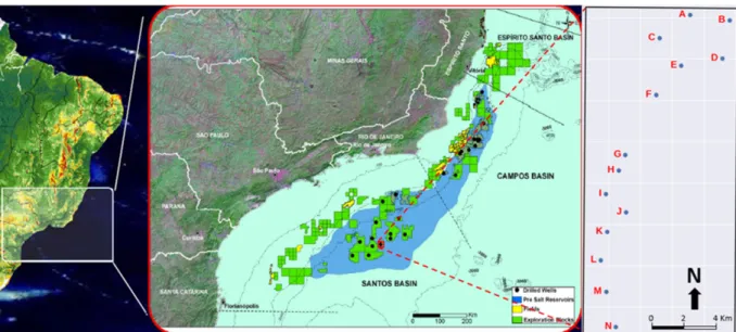
The study area is inserted in the pre-salt province in the Santos and Campos Basins (Fig. 1). A pre-stack depth-migrated volume covering an area of approximately 200 km² is available, together with 14 wells with a broad suite of logs. The Agência Nacional do Petróleo, Gás Natural e Biocombustíveis (ANP) has provided the data we used in this research. Wells were labeled with capital letters from A to N, and the original names can be found in Table 1.
Table 1 – Correspondence between the well symbols for this study and the
official names from ANP (National Agency of Petroleum – Brazil).
This Study ANP
A 3-BRSA-788-SPS B 9-BRSA-1037-SPS C 8-SPH-23-SPS D 8-SPH-13-SPS E 7-SPH-14D-SPS F 7-SPH-8-SPS G 7-SPH-4D-SPS H 9-BRSA-928-SPS I 7-SPH-5-SPS J 9-BRSA-1043-SPS K 1-BRSA-594-SPS L 7-SPH-1-SPS M 7-SPH-2D-SPS N 3-BRSA-923A-SPS
THE IMPORTANCE OF CHARACTERIZATION OF THE EVAPORITIC SECTION
Evaporites are minerals or rocks formed in a restricted saline environment, submitted to high evaporation rates. The great percentage of halite seems to be the main reason to consider the salt section as almost homogenous, with interval velocity Vp close to the halite’s velocity (4,500 m/s), as this is the most frequent mineral within the salt section. However, a look at velocity models obtained by tomographic inversion reveals several inconsistencies, visible in the forms of large spots/marks of different velocities. These marks reflect the necessity to alter the almost constant initial velocity models.
Ji et al. (2011) presented enhanced results of depth positioning in PSDM data when considering seismic amplitudes as the guide for the existing heterogeneity inside the salt section. This improvement alone would be enough to justify the effort of using amplitudes for the velocity modelling. On top of that, it was also noticed that signal quality is improved when using this approach. Gobatto et al. (2016), Fonseca et al. (2018), and Maul et al. (2018a) presented processing results showing that use of salt stratification as input for velocity tomography leads to more realistic seismic images, and to more precise depth positioning and signal quality.
Maul et al. (2015) described how to incorporate salt stratifications using seismic attributes, assigning constant velocity values for those layers. Seismic amplitude is a response of contrasts of elastic properties between rocks. The estimation of layer properties from seismic data is an ill-posed problem (Tarantola, 1984), which bears a set of uncertainties. Seismic inversion is a widely applied technique to combine seismic amplitude, seismic interpretation and well-log information to obtain elastic properties from seismic amplitude (Latimer, 2011). The combination of information from several sources contributes to mitigate the ambiguity of the seismic signal, helping to solve part of the non-uniqueness of the solutions, as observed by Maul et al. (2015).
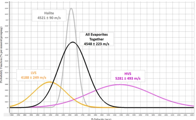
So far, about 200 wells were drilled to access the pre-salt reservoir in the Santos Basin (Maul et al., 2018b). These wells showed that the evaporites are, in fact, heterogeneous, with halite being the major fraction (between 80 and 90%). A division in three mineral groups was proposed: Low-Velocity Salts (LVS), or the bittern salts, composed basically by sylvite, carnallite and tachyhydrite; Halite (or background); and High-Velocity Salts (HVS), which are basically anhydrite and, in lower proportion, gypsum. The LVS group represents something between 5-10%
Figure 1 – Location of study area (regional) and details of available data. Blue polygon delineates the area of the hydrocarbon occurrences identified in the pre-salt
province for both Santos and Campos Basins, totaling an area of approximately 350,000 km², and water column varying from 2,000 to 3,000 m. Rightmost panel shows in detail the well locations (A to N) inside the 3D seismic volume zone (rectangle). Adapted from https://diariodopresal.files.wordpress.com/2010/.
of occurrence, and the HVS group, 10-20%. These groups were considered enough to represent the different observed seismic signatures (Maul et al., 2015; Gobatto et al., 2016; Fonseca et al., 2018; Maul et al., 2018a).
Well-log analysis indicates an inverse relationship between thickness and velocity of the salt section. In areas where the evaporite sequence is thicker, velocity is slower. The Rayleigh-Taylor instability, as described by Lachmann (1910), Arrhenius (1913) and Dooley et al. (2015), can be a physical explanation: it states that under the intense overload pressure caused by the upper sediments, the more mobile salts (LVS) move to high-wall portions. The movement of the low-velocity salts towards the high-wall portions implies in a decrease of velocity in the thicker salt sections, caused by an increase in the fraction of low-velocity salts. This observation is consonant with the one made by Oliveira et al. (2015). The overload pressure moving the mobile salt to the “pillowed” portions is also mentioned by other authors, such as Ge et al. (1997) and Guerra & Underhill (2012).
METHODOLOGY
The proposed methodology in this work consists of:
A. Analysis of the available logs inside the evaporitic section. In this case we observe the presence/absence of data, as well as the property values registered;
B. Precautions regarding the use of samples collected during well drilling, and their associated uncertainties;
C. Interpretation of lithology in the wells, investigating the coupling degree, absence of logs, their description, and their correct positioning;
D. Investigating the property behaviors related to both, their measurement ways as well as considering about anomalous values, their own variability, inferring few commentaries regarding possible compaction effect by each mineral type;
E. Predict properties to insert in log gaps, or where only cuttings description are available. Particularly important for elastic logs;
F. Generation of any other important property for the seismic inversion approach (such as density) using log correlation;
G. Choice of a single and representative wavelet for the whole seismic inversion (in this case, it is important to think about section thickness variation, which could vary from few hundreds of meters to around 3 kilometers); H. Performing a seismic inversion that reproduces the
stratification observed in the well data, for the whole evaporitic section;
I. Obtaining internal stratification for the evaporitic section using other approaches, such as amplitude response, instantaneous seismic attributes, etc.;
J. Comparing the results.
CONSIDERATIONS, ASSUMPTIONS AND DEVELOPMENTS
A frequent challenge when modelling the salt section is the lack of log data at top and bottom of the evaporitic section, which is caused by operational constraints: these two places are usually selected for changing of casing diameter, making it difficult to acquire data from high-resolution acoustic logging. This argument is presented by Amaral et al. (2015), who argues in favor of using sample cuttings to fill this gap in information.
Figure 2 shows information on logs and cutting samples for the 14 studied wells. Notice that well D, for example, does not contain any LVS interpreted in neither approach.
Barros et al. (2017) proposed to use constant values (average logged values) for each of the mineral groups, in order to fill the gaps in the logs – i.e., assuming generated pseudo-logs as hard information. To do so, we will use the following average values: LVS = 4,188 m/s; Halite = 4,548 m/s; and HVS = 5,281. Those values were obtained from the PDF (probability density function) presented in Figure 3.
On the group of wells available for this study, about 10% of the section is not logged – in some cases, log absence is over 20%. Table 2 illustrates the data inventory for the studied wells, as well as some considerations about filling the log gap with the cutting samples description and the average velocity, following Barros et al. (2017).
After complementing the missing log information with the described cuttings, Barros et al. (2017) calculated the average occurrence per proposed group as following: LVS ~ 3.0%, Halite ~ 90.5%, and HVS ~ 6.5%. These percentages are in good agreement with values presented by Jackson et al. (2015) and Maul et al. (2018b), having the latter provided these percentages based on a database of 182 wells in the Santos Basin (Table 3). It is important to point out that the values obtained from this dataset should not be used as reference for any other study.
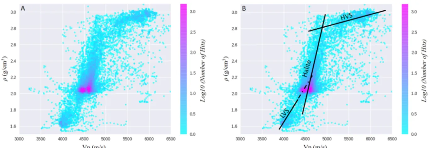
To generate the density logs – another input for the seismic inversion, we employed statistical regressions based on the registered logs (density X sonic), as can be seen in Figure 4.
As previously mentioned, the thickness of the evaporitic section in the Santos Basin varies from few hundreds of meters to about 3 kilometers. This variation imposes challenges when
deciding the single wavelet to perform the seismic inversion process. In this project, the thickness ranges from 1,200 to 2,400 meters, which is enough to produce too different wavelets to be represented for a single average one (Fig. 5). This can compromise the inversion, delivering results that would perhaps be deemed not suitable for reservoir characterization purposes, but still useful for our goals.
RESULTS
The results here presented cover two main aspects: the geological model building, by using the inversion methodology to build the evaporitic section (compared to other methods in literature), and how the use of this approach can influence the generation of new seismic images, depth positioning, migration, and focusing of events.
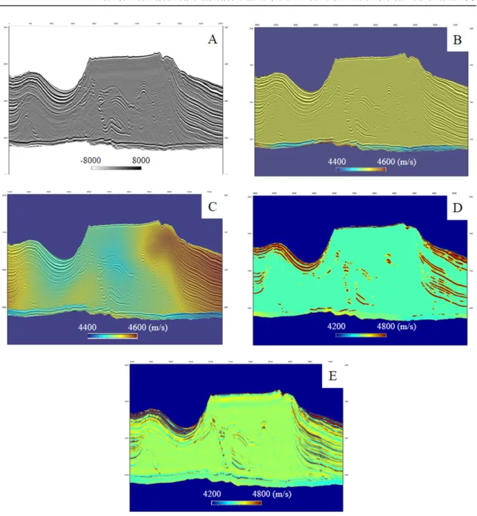
Figure 6A shows a seismic section, illustrating the amplitude responses inside the evaporitic section – the so-called stratifications. Figure 6B shows a velocity model with constant velocity for the evaporitic section (4,500 m/s), which was used as input for tomography, yielding the velocity presented in Figure 6C. If we use the amplitude response (Fig. 6A) to add stratification to the tomography output, we get a more geological look in our model, as can be seen in Figure 6D. Figure 6E shows the velocity obtained with the seismic inversion methodology.
The seismic inversion result is an impedance cube, and we are looking for an interval velocity cube. Following the idea showed in Figure 4, we can compute the correlation between impedance and interval velocity in well data. This was done independently for each of the three salt groups, using linear regressions, and the resulting equations were applied to the acoustic impedance obtained from inversion, yielding the desired 3D interval velocity.
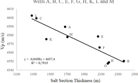
The results show the inverse correlation between average interval velocity and section thickness (Fig. 7), for 10 of the 14 wells. This behavior was not observed in the remaining 4 wells. We believe this can be caused by problems in log data from these wells – the inverse relation is also described by Oliveira et al. (2015) after studying only three wells in another portion of in the Santos Basin, and by Maul et al. (2018b), in a study of 182 wells. It is in fact possible to use the impedance results to verify the same behavior spatially, as in Figure 8. This subject is currently in discussion and will likely be the scope of future work.
In another way, using Table 3 it is also possible to observe different behaviors when analyzing separately each mineral grouping per well. It allows us to infer when staying in thin
Figure 2 – Well section illustrating the registered logs and drill cuttings interpretation. Observe the absence of log information in almost all 14 wells.
Table 2 – Well data inventory.
EKB Basal Water Top Salt Acquired Log LVS Halite HVS AIV Anhy- Column of Salt Isopach Log Gap Log & Log & Log & Velocity
drite TVDSS TVDSS C.S. C.S. C.S. Well (m) (m) (m) (m) (m) ( %) ( %) (%) (%) (%) (m/s) A 25.00 12.90 -2125.00 -3264.81 1673.49 91.90 8.10 5.45 86.20 8.35 4589.59 B 24.00 13.80 -2122.00 -2734.32 2369.39 87.60 12.40 0.50 98.90 0.60 4550.39 C 24.00 12.90 -2146.00 -3722.50 1334.06 91.10 8.90 6.90 82.70 10.40 4599.39 D 24.00 11.50 -2119.00 -2717.34 2400.94 87.30 12.70 0.00 91.60 8.40 4609.57 E 24.00 11.14 -2179.00 -2885.90 2063.00 77.90 22.10 0.30 95.40 4.30 4578.44 F 24.00 17.50 -2182.00 -2876.91 2081.76 87.20 12.80 1.45 95.40 3.15 4565.87 G 24.00 13.57 -2129.00 -2804.89 2180.45 92.00 8.00 4.80 92.90 2.30 4547.58 H 24.00 11.50 -2120.00 -2798.11 2191.82 91.80 8.20 1.20 98.10 0.70 4548.81 I 26.00 13.80 -2126.00 -2809.53 2206.90 91.40 8.60 1.10 88.80 10.10 4618.07 J 26.00 13.40 -2140.00 -3088.84 2024.65 96.00 4.00 5.10 83.80 11.10 4611.00 K 32.00 11.50 -2140.00 -3553.21 1450.89 98.40 1.60 2.12 93.10 4.78 4575.41 L 26.00 29.40 -2143.00 -3717.59 1279.96 95.60 4.40 3.60 87.20 9.20 4602.48 M 26.00 11.65 -2143.00 -3256.49 1701.27 94.30 5.70 4.10 89.80 6.10 4577.95 N 26.00 13.30 -2157.00 -3340.66 1717.34 94.00 6.00 4.60 83.20 12.20 4620.87 AVG 25.36 14.13 -2140.79 -3112.22 1905.42 91.18 8.82 2.94 90.51 6.55 4585.39 EKB: Elevation Kelly-Bushing; TVDSS: True Vertical Depth Sub-Sea; LVS: Low-Velocity Salts; HVS: High-Velocity Salts; C.S.: Cutting Samples;
AVG: Average; AIV: Average Interval Velocity.
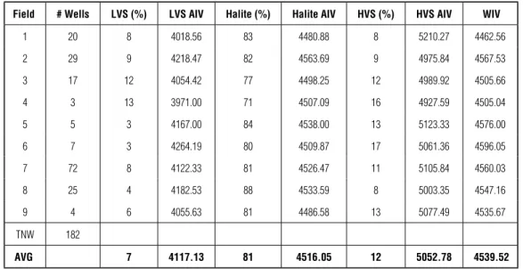
Table 3 – Salt proportions and interval velocities (m/s) for nine fields inside Santos Basin.
Field # Wells LVS (%) LVS AIV Halite (%) Halite AIV HVS (%) HVS AIV WIV
1 20 8 4018.56 83 4480.88 8 5210.27 4462.56 2 29 9 4218.47 82 4563.69 9 4975.84 4567.53 3 17 12 4054.42 77 4498.25 12 4989.92 4505.66 4 3 13 3971.00 71 4507.09 16 4927.59 4505.04 5 5 3 4167.00 84 4538.00 13 5123.33 4576.00 6 7 3 4264.19 80 4509.87 17 5061.36 4596.05 7 72 8 4122.33 81 4526.47 11 5105.84 4560.03 8 25 4 4182.53 88 4533.59 8 5003.35 4547.16 9 4 6 4055.63 81 4486.58 13 5077.49 4535.67 TNW 182 AVG 7 4117.13 81 4516.05 12 5052.78 4539.52
LVS: Low-Velocity Salts; HVS: High-Velocity Salts; AIV: Average Interval Velocity; WIV: Weighted Interval Velocity; TNW: Total Number of Wells; Interval Velocity (m/s); AVG: Average. Modified from Maul et al. (2018b).
Figure 4 – Relation between density and instantaneous velocity (Vp). (A) Density X Interval Velocity; (B) Trend line for each proposed group (LVS, Halite and HVS).
Notice that the Halite trend is more stable than the others. This is not surprising, since the other groups are in fact a mixing of minerals, while Halite – despite any mixing – has a monomineralic behavior.
Figure 5 – Best wavelets for each of the 14 wells, and the average among them (purple). Observe the low representation of the average wavelet compared with the
individual ones.
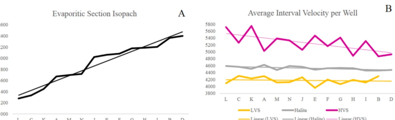
section we preferably have an increase in the HVS content or proportions which is reflected in the interval velocity increasing in these portions (Fig. 9). A feasible explanation is the fact during the period of more mobility observed for the Halite and the LVS, these salts under any overpressure condition tend to move to a any low-pressure portion such as the walls, pillows increasing their amounts in those places which consequently decreasing their velocity content. Another important aspect is the mineral mixing promotion during this moving which as per Justen et al. (2013)
statement helps to explain why the halite velocity is commonly measured below the value of 4,500 m/s, once the measurement reflects also the LVS content.
With the velocity models in hands, we can compare the output of processing workflows under different inputs. In this project, tomography and Kirchhoff PSDM were tested, using both the constant velocity model (Fig. 6B) and the impedance-derived one (Fig. 6E) as initial models. Results can be checked in Figure 10.
Figure 6 – The evaporitic section and the velocity behaviors in terms of geological features. (A) amplitude response; (B) constant interval velocity; (C) tomographic
update in terms of velocity applied over “4B”, which generated “4A”; (D) stratification insertion using the amplitude “4A” as the guide for this insertion; (E) stratification insertion using the seismic inversion methodology.
DISCUSSION
One hypothesis investigated during this research was that evaporitic sections show higher velocities in thin sections than in thicker sections. Results obtained from seismic inversion – even with a challenging wavelet estimation – are in agreement
with this. This assumption could also be inferred by observing the local geology, particularly the mini-basins under carbonate rafts: the heavy sediments in those mini-basins force the LVS to move to other positions, forming domes and walls. Therefore, the thin sections are left with a higher fraction of HVS, explaining their higher velocity.
Figure 7 – Correlation between average interval velocity and salt thickness for the evaporitic section
(10 of 14 wells displayed).
Figure 8 – Comparison between average interval velocity and thickness for the evaporitic section. (a) map of
average interval velocity for the evaporitic section, with location of available wells (velocities were calculated from impedance volume); (b) map of thickness. Notice the same trend found in the cross-plot in Figure 7: thicker layers have slower interval velocity.
Figure 9 – Thickness section variation and the impact it may cause for each mineral/grouping. (A) thickness variation from the thinner section to the thicker; (B) average
interval velocity per mineral/grouping per well. Note the influence the thickness appears to have of the HVS.
Figure 10 – Comparison between Kirchhoff migration with the tomographic updated for a constant initial model (Vp = 4,500 m/s) and for model with stratification. (A)
migrated Kirchhoff crossline using the traditional tomographic updating for the velocity model (starting model Vp = 4,500 m/s); (B) the same crossline migrated using the Kirchhoff algorithm, now using the tomographic updating over the stratified model; (C) migrated Kirchhoff inline using the traditional tomographic updating for the velocity model (starting model Vp = 4,500 m/s); (D) the same inline migrated using the Kirchhoff algorithm, now using the tomographic updating over the stratified model. Orange arrows indicate positions where we observed imaging enhancement. Adapted from Maul et al. (2018a).
Imaging enhancement has been reported in recent literature when accounting for stratification prior to tomography (Gobatto et al., 2016; Fonseca et al., 2017; Fonseca et al., 2018; Maul et al. 2018b). Besides better depth positioning and uncertainty reduction, event focusing is also improved. On this particular subject, there is plenty of room for development – the use of Least-Squares Migration (LSM), for example. These are the next steps in our research.
CONCLUSION
Seismic inversion for the evaporitic section is a suitable approach to start building reliable velocity models, even when the inversion output is not up to the standards of reservoir characterization. Using a stratified velocity as initial model for tomography update delivers clear benefits for the processing workflow, by reducing the computational time necessary for this intensive step. This is mostly due to incorporation of geology into the model, which brings it closer to the optimal solution and trims the number of necessary iterations.
The inverse relation between the evaporitic section thickness and its average interval velocities reinforces the mobile salts (LVS and Halite) expulsion hypothesis. Therefore, the HVS proportion is higher in thin sections. This is sometimes observed in thinner salt sections from tomographic updates of constant initial models, even without any geological input.
Both imaging and depth positioning are improved by using the stratified velocity model for tomography. These improvements can be carried even further by the use of migration algorithms that make better use of detailed velocity models, like Least-Squares Migration. Also, several other tasks can take advantage of better salt characterization, such as illumination studies, geomechanical simulations, and HSE during drilling operations.
AMARAL PJ, MAUL A, FALCÃO L, GONZÁLEZ M & GONZÁLEZ G. 2015. Estudo Estatístico da Velocidade dos Sais na Camada Evaporítica na Bacia de Santos. In: 14th International Congress of the Brazilian Geophysical Society. Rio de Janeiro, RJ, Brazil. doi: 10.1190/sbgf2015-131.
ARRHENIUS S. 1913. Zur Physik der Salzlagerstätten. Medd. Vetensskapsakademiens Nobelinst, 2(20): 1-25.
BARNES C & CHARARA M. 2009. The Domain of Applicability of Acoustic Full-Waveform Inversion for Marine Seismic Data. Geophysics, 74(6): WCC91–WCC103. doi: 10.1190/1.3250269.
BARROS P, FONSECA J, TEIXEIRA L, MAUL A, YAMAMOTO T, MENEGUIM T, QUEIROZ LE, TORÍBIO T, MARTINI A, GOBATTO F & GONZÁLEZ M. 2017. Salt Heterogeneities Characterization in Pre-Salt Santos Basin Fields. In: OTC Brasil, Offshore Technology Conference. Rio de Janeiro, RJ, Brazil: IBP. doi: 10.4043/28147-MS.
BEN-HADJ-ALI H, OPERTO S & VIRIEUX J. 2008. Velocity Model Building by 3D Frequency-Domain, Full-Waveform Inversion of Wide-Aperture Seismic Data. Geophysics, 73(5): VE101-VE117. doi: 10.1190/1.2957948.
CORNELIUS S & CASTAGNA JP. 2018. Variation in Salt-Body Interval Velocities in the Deepwater Gulf of Mexico: Keathley Canyon and Walker Ridge Areas. Interpretation, 6(1): T15-T27. doi: 10.1190/INT-2017-0069.1.
DIAS BP, BULCÃO A, SOARES FILHO DM, SANTOS LA, DIAS RM, LOUREIRO FP & DUARTE FS. 2017. Least-Squares Migration in the Image Domain with Sparsity Constraints: an Approach for Super-Resolution in Depth Imaging. In: 15th International Congress of the Brazilian Geophysical Society. Expanded Abstracts. Rio de Janeiro, RJ, Brazil. doi: 10.1190/sbgf2017-236.
DIAS BP, GUERRA C, BULCÃO A & DIAS RM. 2018. Exploring Inversion Strategies in Image Domain Least Squares Migration. In: First EAGE/SBGf Workshop on Least Squares Migration. LMSTU01. Rio de Janeiro, RJ. Brazil. doi: 10.3997/2214-4609.201803060.
DOOLEY TP, JACKSON MPA, JACKSON CA-L, HUDEC MR & RODRIGUEZ CR. 2015. Enigmatic Structures within Salt Walls of Santos Basin – Part 2: Mechanical Explanation from Physical Modeling. Journal of Structural Geology, 75: 163-187. doi: 10.1016/j.jsg.2015.01.009. FONSECA J, GOBATTO F, BOECHAT J, MAUL A, YAMAMOTO T, BORN E, TEIXEIRA L & GONZÁLEZ M. 2017. Dealing with Evaporitic Salts Section in Santos Basin during Geological Seismic Velocity Construction. In: 15th International Congress of the Brazilian Geophysical Society. Expanded Abstracts. Rio de Janeiro, RJ, Brazil. doi: 10.1190/sbgf2017-350.
FONSECA J, TEIXEIRA L, MAUL A, BARROS P, BOECHAT J & GONZÁLEZ M. 2018. Modelling Geological Layers into new Velocity Models for Seismic Migration Process: A Brazilian pre-salt Case. In: First EAGE/PESGB Workshop on Velocities. London, United Kingdom. doi: 10.3997/2214-4609.201800010.
GE H, JACKSON MPA & VENDERVILLE BC. 1997. Kinematics and Dynamics of Salt Tectonics Driven by Propagation. American Association of Petroleum Geologists Bulletin, Tulsa, Oklahoma, 81: 398-423. GOBATTO F, MAUL A, FALCÃO L, TEIXEIRA L, BOECHAT JB, GONZÁLEZ M & GONZÁLEZ G. 2016. Refining Velocity Model within the Salt Section in Santos Basin: an Innovative Workflow to include the Existing Stratification and its Considerations. In: 86th Annual Meeting. SEG – Society of Exploration Geophysicist. Dallas, TX, USA. doi: 10.1190/segam2016-13685489.1.
GUERRA MCM & UNDERHILL JR. 2012. Role of Halokinesis in Controlling Structural Styles and Sediment Dispersal in the Santos Basin, Offshore Brazil. In: ALSOP GI, ARCHER SG, HARTLEY AJ, GRANT NT & HODGKINSON R (Eds.). Salt Tectonics, Sediments and Prospectivity. Geol. Soc. London, Special Public., 363: 175-206. doi: 10.1144/SP363.9.
HSÜ K. 1972. Origin of Saline Giants: A Critical Review after the Discovery of the Mediterranean Evaporite. Earth-Science Reviews, 8: 371–396. doi: 10.1016/0012-8252(72)90062-1.
HU J, SCHUSTER GT & VALASEK PA. 2001. Post-Stack Migration Deconvolution. Geophysics, 66: 939-952. doi: 10.1190/1.1444984. HUANG Y, LIN D, BAI B, ROBY S & RICARDEZ C. 2010. Challenges in Pre-Salt Depth Imaging of the Deepwater Santos Basin, Brazil. The Leading Edge, 29(7): 820–825. doi: 10.1190/1.3462785.
HÜBSCHER C, CARTWRIGHT J, CYPIONKA H, DE LANGE GJ, ROBERTSON A, SUC J-P & URAI JL. 2007. Global Look at Salt Giants: Eos (Transactions, American Geophysical Union), 88: 177–182. doi: 10.1029/2007EO160002.
JACKSON CA-L, JACKSON MPA, HUDEC MR & RODRIGUEZ CR. 2015. Enigmatic Structures within Salt Walls of Santos Basin – Part 1: Geometry and Kinematics from 3D Seismic Reflection
and Well Data. Journal of Structural Geology, 75: 135-162. doi: 10.1016/j.jsg.2015.01.010.
JI S, HUANG T, FU K & LI Z. 2011. Dirty Salt Velocity Inversion: The Road to a Clearer Subsalt Image. Geophysics, 76(5): WB169–WB174. doi: 10.1190/GEO2010-0392.1.
JUSTEN JCR, VARGAS Jr EA, ALVES I & SOUZA ALS. 2013. Análise das Propriedades Elásticas de Rochas e Minerais Evaporíticos. In: 13th International Congress of Brazilian Geophysical Society. Rio de Janeiro, RJ, Brazil. doi: 10.1190/sbgf2013-237.
LACHMANN R. 1910. Über Autoplaste (Nichttektonische) Formelemente im Bau der Salzlagerstätten Norddeutschlands. Z. Dtsch. Geol. Ges., 62: 113-116.
LATIMER RB. 2011. Inversion and Interpretation of Impedance Data. In: BROWN AR. Interpretation of Three-Dimensional Seismic Data. Society of Exploration Geophysicists and American Association of Petroleum Geologists, Tulsa, Oklahoma, USA. p. 309–350. doi: 10.1190/1.9781560802884.ch9.
MAUL A, JARDIM F, FALCÃO L & GONZÁLEZ G. 2015. Observing Amplitude Uncertainties for a pre-salt Reservoir using Illumination Study (Hit-Maps). In: 77th EAGE Conference & Exhibition. Madrid, Spain. doi: 10.3997/2214-4609.201412921.
MAUL A, FONSECA J, TEIXEIRA L, BARROS P, BOECHAT JB, NUNES JP, YAMAMOTO T, GONZÁLEZ M & GONZÁLEZ G. 2018a. Modelling Intra-Salt Layers when Building Velocity Models for Depth Migration. Examples of the Santos Basins, Brazilian Offshore. In: 88th Annual Meeting. SEG – Society of Exploration Geophysicist. Anaheim, CA, USA. doi: 10.1190/segam2018-2996209.1.
MAUL A, SANTOS MAC & SILVA CG. 2018b. Evaporitic Section Characterization and its Impact over the pre-salt Reservoirs, Examples in Santos Basin, Offshore. In: Rio Oil & Gas Expo & Conference 2018. Rio de Janeiro, RJ, Brazil. IBP.
MAUL AR, SANTOS MAC & SILVA CG. 2018c. Few Considerations, Warnings and Benefits for the E&P Industry when Incorporating Stratifications inside Salt Sections. Brazilian Journal of Geophysics, 36(4): 461-477. doi: 10.22564/rbgf.v36i4.1981.
MENEGUIM T, MENDES SC, MAUL A, FALCÃO L, GONZÁLEZ M & GONZÁLEZ G. 2015. Combining Seismic Facies Analysis and Well Information to Guide new Interval Velocity Models for a pre-salt Study, Santos Basin, Brazil. In: 14th International Congress of the Brazilian Geophysical Society. Rio de Janeiro, RJ, Brazil. doi: 10.1190/sbgf2015-271.
NEMETH T, WU C & SCHUSTER GT. 1999. Least-Squares Migration of Incomplete Reflection Data. Geophysics, 64: 208–221. doi: 10.1190/1.1444517.
M. 2018. Dual Tectonic-Climatic Controls on Salt Giant Deposition in the Santos Basin, Offshore Brazil. Geosphere, 14(1): 215-242. doi: 10.1130/GES01434.1.
SCHREIBER BC, BABEL M & LUGLI S. 2007. An Overview of Evaporite Puzzles. In: SCHREIBER BC, LUGLI S & BABEL M (Eds.). Evaporites through Space and Time. Geological Society, London, Special Publication, 285. doi: 10.1144/SP285.2.
SIMM R & BACON M. 2014. Seismic Amplitude: An Interpreter’s Handbook. Cambridge Press. 271 pp.
STEFANO L, MANZI V, ROVERI M & SCHREIBER BC. 2010. The Primary Lower Gypsum in the Mediterranean: A new Facies Interpretation for the First Stage of the Messinian Salinity Crisis. Palaeogeography, Palaeoclimatology, Palaeoecology, 297: 83–99. doi: 10.1016/j.palaeo.2010.07.017.
and Geomechanical Properties using Seismic Inversion, a Case Study for Santos Basin. In: 15th International Congress of the Brazilian Geophysical Society. Rio de Janeiro, RJ, Brazil. doi: 10.1190/sbgf2017-226.
VIGH D, JIAO K, WATTS D & SUN D. 2014. Elastic Full-Waveform Inversion Application using Multicomponent Measurements of Seismic Data Collection. Geophysics, 79(2): R63–R77. doi: 10.1190/geo2013-0055.1.
WANG P, HUANG H & WANG M. 2017. Improved Subsalt Images with Least-Squares Reserve Time Migration. Interpretation, 5(3): SN25-SN32. doi: 10.1190/INT-2016-0203.1.
ZHANG Y & WANG D. 2009. Traveltime Information-Based Wave-Equation Inversion. Geophysics, 74(6): WCC27–WCC36. doi: 10.1190/1.3243073.
Recebido em 11 fevereiro, 2019 / Aceito em 22 março, 2019 Received on February 11, 2019 / accepted on March 22, 2019