Repositório ISCTE-IUL
Deposited in Repositório ISCTE-IUL:2019-05-20
Deposited version:
Post-print
Peer-review status of attached file:
Peer-reviewed
Citation for published item:
Ferreira-Lopes, A. & Sequeira, T. N. (2014). The dynamics of the trade balance and the terms of trade in Central and Eastern European countries. Acta Oeconomica. 64 (1), 51-71
Further information on publisher's website:
10.1556/AOecon.64.2014.1.3
Publisher's copyright statement:
This is the peer reviewed version of the following article: Ferreira-Lopes, A. & Sequeira, T. N. (2014). The dynamics of the trade balance and the terms of trade in Central and Eastern European countries. Acta Oeconomica. 64 (1), 51-71, which has been published in final form at
https://dx.doi.org/10.1556/AOecon.64.2014.1.3. This article may be used for non-commercial purposes in accordance with the Publisher's Terms and Conditions for self-archiving.
Use policy
Creative Commons CC BY 4.0
The full-text may be used and/or reproduced, and given to third parties in any format or medium, without prior permission or charge, for personal research or study, educational, or not-for-profit purposes provided that:
• a full bibliographic reference is made to the original source • a link is made to the metadata record in the Repository • the full-text is not changed in any way
The full-text must not be sold in any format or medium without the formal permission of the copyright holders.
Serviços de Informação e Documentação, Instituto Universitário de Lisboa (ISCTE-IUL) Av. das Forças Armadas, Edifício II, 1649-026 Lisboa Portugal
The Dynamics of the Trade Balance and the
Terms of Trade in Central and Eastern
European Countries
Alexandra Ferreira-Lopes
∗and Tiago Neves Sequeira
†Abstract
In this work we assess the existence of a S-Curve pattern in ten Cen-tral and Eastern European Countries (CEEC-10) for the relation between the trade balance and the terms of trade. Empirical results support the existence of this curve for Slovenia, Czech Republic, Hungary, and also for an aggregate of the ten transition countries. In the case of Lithuania, Poland, Romania, and Slovakia the pattern is weaker than in the men-tioned countries but it stills prevails. We then document this property of business cycles in the dynamic general equilibrium trade model of Backus, Kehoe, and Kydland (1994) calibrated specifically to match the CEEC-10 aggregate economy. Results support the existence of a S-Curve, except when technology shocks are absent and domestic and imported goods are perfect substitutes.
JEL Classification: C68, F32, F41.
Keywords: Central and Eastern European Countries, Current Account Dy-namics, Terms of Trade, S-Curve.
∗ISCTE (Lisbon University Institute), Economics Department, Economics Research Center
(ERC)-UNIDE, and DINÂMIA. Avenida das Forças Armadas, 1649-026 Lisboa, Portugal. Tel.: +351 217903901; Fax: +351 217903933; E-mail: [email protected]
†UBI and INOVA, UNL. [email protected]. Management and Economics Department.
Uni-versidade da Beira Interior. Estrada do Sineiro, 6200-209 Covilhã, Portugal. Tiago Neves Sequeira acknowledges the financial support from POCI/FCT.
1
Introduction
In this work we empirically assess the existence of a S-Curve relation between the terms of trade (or the real exchange rate) and net exports in ten Central and Eastern European Countries (CEEC-10), and analyze our empirical findings, calibrating the dynamic general equilibrium trade model of Backus, Kehoe, and Kydland (1994) to match parameter values for an aggregate (CEEC-10) of the economies at study.
Before we characterize a S-Curve pattern, we must first define a related con-cept - The J-Curve. The J-Curve phenomenon is observed in the data when the trade balance of a given country gets worse immediately after a real currency depreciation, due to some time lag between order and delivery of imports, which are paid on a higher price after the depreciation. Empirical studies have revealed that in developed economies this event usually lasts between 6 month and one year. Hence the existence of a J-Curve makes realignments in exchange rates less predictable, increasing the volatility and uncertainty, especially regarding the consequences on output, export competitiveness, and real convergence. Sem-inal studies about the J-Curve can be traced back to the works of Junz and Rhomberg (1973), Magee (1973), and Meade (1988). The S-Curve pattern as mentioned in the work of Backus, Kehoe, and Kydland (1994) is a similar defin-ition to the J-Curve, but instead of only studying the existence of negative past and contemporaneous correlations between the terms of trade and net exports, in order for a S-Curve pattern to exist, positive correlations between the two variables must emerge in the future.
The ten Central and Eastern European Countries (CEEC-10) which in recent years joined the European Union (EU) — Bulgaria, Czech Republic, Estonia, Hungary, Latvia, Lithuania, Poland, Romania, Slovakia, and Slovenia - are going through a transition process, being the ultimate goal real convergence towards EU levels. The study of the S-Curve phenomenon for these countries is useful for several reasons. First, uncertainty about the impact of exchange rates depreciations caused by the existence of a S-Curve in these small open economies can undermined the convergence process, since economic growth in
recent years for these countries is mostly export-oriented. Second, since these economies have, sooner or later, to join the euro, constant depreciations and uncertainty about their final impact on the economy, can potentially increase volatility in their transition path towards the euro. Third, the timing of euro adoption or even the entrance in to the Exchange Rate Mechanism (ERM II) can be more difficult to pin down since volatility of exchange rates, its impact on the economy, and constant deficits in the trade balance are reasons to delay those decisions.
Literature about transition countries at study and the connection between the trade balance and the terms of trade is still very scarce and empirical. Some studies focused mainly on determinants of the current account, for example Herrman and Jochem (2005), Falk (2008), and Rahman (2008).
Herrman and Jochem (2005) study the determinants of current account in the Central and Eastern Europe Countries (except Bulgaria and Romania, the other eight are the ones we study) and its impact for euro zone enlargement. Among other conclusions, the authors are concerned about future realignments of real exchange rates that can potentially harm the timing and the certainty of the determination of the conversion rate to the euro. Falk (2008) using a sample of 32 countries between 1990 and 2007, including our ten transition countries, analyzed the determinants of the trade balance in these countries. This work does finds a positive connection between a real exchange rate depreciation and an improvement in the trade balance (contrary to the S-Curve), although countries with trade balance deficits and/or large inflows of foreign direct investment become less sensitive to movements in real exchange rates. Rahman (2008) also analyzes our ten economies between 1992 and 2006, trying to understand recent developments in the current account in these countries using several variables as possible causes.
Other studies focus mostly on the impact of exchange rates on economic growth. Kemme and Teng (2000) find evidence that misalignments in real ex-change rates tend to undermine export growth in Poland. Égert and Morales-Zumaquero (2008) found evidence of the same but for the case of nominal
ex-change rates across ten Central and Eastern European countries. Bahmani-Oskooee and Kutan (2008a) try to assess, for seven of our ten economies (ex-cept Bulgaria, Romania, and Slovenia) if exchange rate depreciations are output contractionary or not. They find that in the short-run a depreciation benefits Latvia, Poland, and Slovakia, since exports are reacting more, but is harmful for Czech Republic, Estonia, and Hungary, having no effect in Lithuania.
The two empirical studies that clearly analyze the existence (or not) of the referred phenomenon for the CEEC are Bahmani-Oskooee and Kutan (2008b) and Bahmani-Oskooee, Kutan, and Ratha (2008c). The first study uses monthly data for the period between January 1990 and June 2005 for, among others, Bulgaria, the Czech Republic, Hungary, Poland, Romania, and Slovakia. For our selection of countries, the author finds evidence of a J-Curve for Bulgaria. The second study uses the same data to test the existence of an S-Curve instead of an J-Curve (i.e., instead of only analyzing the existence of a negative relationship between the real exchange rate and the trade balance in the first periods after a depreciation, the authors also assess if after some periods their relationship turns positive). Again, results for Bulgaria show evidence of a S-Curve, as well as for Poland, and Slovakia. Weak evidence is found for Czech Republic and Hungary.
In this work, besides contributing to the increasing empirical literature about the connection between the terms of trade and net exports, we also analyze this relation for Central and Eastern European Countries in a dynamic general equi-librium trade setting, calibrated specifically to replicate economic characteristics for an aggregate of these countries (CEEC-10). This framework has never been used in the literature to study this topic for the case of these countries.
In the next section we will present empirical motivation for the ten countries at study. Section 3 presents the model and section 4 the calibration exercise for these countries. Section 5 analyzes the results of the benchmark and robust-ness analysis simulations, and compares those with empirical evidence found in section 2. Finally, section 6 concludes.
2
Empirical Motivation
Table 1 shows indicators regarding convergence and trade for the ten Central and Eastern European Countries that recently join the European Union. Com-parison of GDP per capita is made with Germany and the import share in % of GDP represent imports of each country that come from Germany. We choose Germany for comparison purposes since the country is the biggest economy in the European Union.
Table 1 - Convergence and Trade R elated Indicators
GDP Per Capita Degree of Import Share Trade Balance
(Germany=100) Openness (in % GDP) (% GDP)
Bulgaria 34.5 74.4 8.8 −22.1 Czech Republic 71.4 76.6 19.8 4.7 Estonia 63.2 77.2 10.0 −8.9 Hungary 56.4 78.8 17.8 2.3 Latvia 50.9 54.5 8.5 −20.3 Lithuania 49 61.4 8.7 −12.0 Poland 47.3 42.1 10.7 −1.7 Romania 32.3 37.6 7.5 −14.3 Slovakia 58.3 86.6 17.4 −0.5 Slovenia 79.9 72.3 11.5 −1.8 D a t a S o u r c e s : N e w C r o n o s ( E u r o s t a t ) a n d C h e l e m . A l l v a l u e s p r e s e n t e d r e f e r t o 2 0 0 7 , e x c e p t f o r t h e c a s e o f t h e i m p o r t s h a r e , w h i c h i s 2 0 0 6 . D e g r e e o f o p e n n e s s i s c a l c u l a t e d a s [ ( E x p o r t s + I m p o r t s ) / 2 ] / G D P * 1 0 0 a t c u r r e n t p r i c e s . I m p o r t s h a r e i n % o f G D P i s c a l c u l a t e d w i t h i m p o r t s f r o m G e r m a n y f o r e a c h c o u n t r y a t c u r r e n t p r i c e s . T r a d e b a l a n c e i s ( E x p o r t s - I m p o r t s ) / G D P * 1 0 0 i n c u r r e n t p r i c e s .
These ten countries are on different stages of convergence towards Germany, with Bulgaria and Romania being the poorest and the newest members of the European Union, as we can see by analyzing GDP per capita in % of Germany GDP per capita. All countries have a substantial degree of openness making these small open economies very dependent of the economic conditions of their trade partners, which can also be confirmed by looking at the column where the trade balance as a % of GDP is presented. Countries like Bulgaria, Es-tonia, Latvia, Lithuania, and Romania show worrying values for their trade balances deficits, exposing a significant foreign dependence. Imports from Ger-many already represent a significative value for these countries (and exports also, although results are not presented).
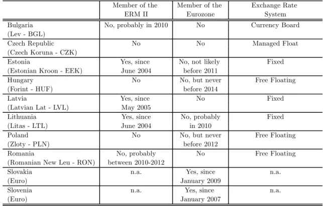
Table 2 show us the current situation in each of this ten countries regarding exchange rate policy. Only two of the ten transition countries are already in
the Eurozone - Slovenia and Slovakia. However, there are three countries that are already inside the Exchange Rate Mechanism II (ERM II) controlling the volatility of its currencies - Estonia, Latvia, and Lithuania - making a serious effort about joining the Eurozone. Czech Republic, Hungary, Poland, Bulgaria, and Romania, the biggest transition economies are still outside the ERM II and very undecided about time schedules.
Table 2- Exchange R ate Policy
Member of the Member of the Exchange Rate
ERM II Eurozone System
Bulgaria No, probably in 2010 No Currency Board
(Lev - BGL)
Czech Republic No No Managed Float
(Czech Koruna - CZK)
Estonia Yes, since No, not likely Fixed
(Estonian Kroon - EEK) June 2004 before 2011
Hungary No No, but never Free Floating
(Forint - HUF) before 2014
Latvia Yes, since No Fixed
(Latvian Lat - LVL) May 2005
Lithuania Yes, since No, probably Fixed
(Litas - LTL) June 2004 in 2010
Poland No No, but never Free Floating
(Zloty - PLN) before 2012
Romania No, probably No Free Floating
(Romanian New Leu - RON) between 2010-2012
Slovakia n.a. Yes, since n.a.
(Euro) January 2009
Slovenia n.a. Yes, since n.a.
(Euro) January 2007
Data Sources: National Central Bank of each country. ERM II is the Exchange Rate Mechanism II.
The name of the currency is in parentheses as well as its international designation in foreign exchange markets.
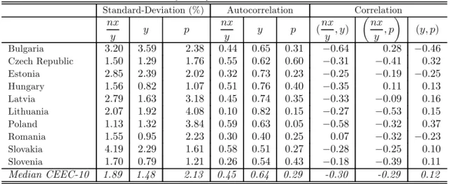
Table 3 presents calculations similar to those of Backus, Kehoe, and Kyd-land (1994) for the ten transition countries, using quarterly data. Variables
used in this table are similar to variables that we used in the model. nxy is net
exports in % of GDP at current prices, y is GDP at constant prices, and p is the terms of trade, calculated as the ratio of the implicit import deflator over the implicit export deflator, contrary to the standard definition used in inter-national economics, but in line with the definition of real exchange rates used
in macroeconomics.1 The last row of this table shows the median of the values
found, this median represents a value for the aggregate of the ten transition countries (CEEC-10), which we use to compare the model against empirical data in section 5.
In terms of standard deviations all variables exhibit a considerable amount of volatility, especially in the case of the terms of trade, but values are rather
heterogeneous across countries. nx
y and y are the most persistent variables while
the terms of trade presents a rather small median value of 0.29.
Correlations between y and nxy are always negative, at the exception of
Romania, as it is standard in the literature, emphasizing the strong connection between income and imports. The correlation between GDP and the terms of trade does not present a clear trend, but it is, most of the time, positive. In eight of our ten countries (except Bulgaria and Hungary) the contemporaneous correlation between net exports and the terms of trade is negative. This means that whenever there is a real depreciation, the trade balance worsens, which can be an evidence of the existence of a S-Curve phenomenon in these countries.
Table 3 - Business Cycle Prop erties of the Ten Transition Econom ies
Standard-Deviation (%) Autocorrelation Correlation
nx y y p nx y y p ( nx y , y) µ nx y , p ¶ (y, p) Bulgaria 3.20 3.59 2.38 0.44 0.65 0.31 −0.64 0.28 −0.46 Czech Republic 1.50 1.29 1.76 0.55 0.62 0.60 −0.31 −0.41 0.32 Estonia 2.85 2.39 2.02 0.32 0.73 0.23 −0.25 −0.19 −0.25 Hungary 1.56 0.82 1.07 0.51 0.76 0.40 −0.35 0.11 0.13 Latvia 2.79 1.63 3.18 0.45 0.74 0.35 −0.33 −0.09 0.16 Lithuania 2.07 1.92 4.08 0.10 0.82 0.15 −0.27 −0.53 0.15 Poland 1.13 1.32 3.84 0.59 0.63 0.05 −0.58 −0.32 0.37 Romania 1.55 0.95 2.23 0.30 0.40 0.25 0.07 −0.32 −0.23 Slovakia 4.19 2.29 1.61 0.58 0.51 0.27 −0.28 −0.25 0.10 Slovenia 1.70 0.79 1.21 0.26 0.54 0.43 −0.18 −0.39 0.11 Median CEEC-10 1.89 1.48 2.13 0.45 0.64 0.29 -0.30 -0.29 0.12
Notes: Quarterly data is from the NewCronos (Eurostat) database. Authors’ own calculations.
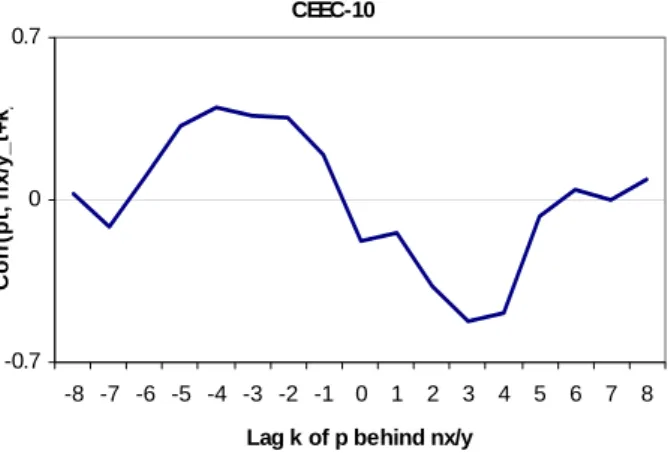
To better assess the connection between net exports and the terms of trade
we calculated correlations between the two variables, i.e., pt and (nxy )t+k for
lags and leads of 8 periods each, which can be seen in Figure 1.
A S- pattern emerges in Slovenia, Czech Republic, and Hungary. In the case of Lithuania, Poland, Romania, and Slovakia the pattern is weaker than in
the mentioned three countries, but the evolution is the same, getting positive correlations after k = 0. Results for Bulgaria, Estonia, and Latvia seem to indicate that the pattern does not appear in these countries. Except for the case of Bulgaria, conclusions are relatively similar to the ones in Bahmani-Oskooee and Kutan (2008b) and Bahmani-Bahmani-Oskooee, Kutan, and Ratha (2008c), although they use monthly data.
S lo ve n ia - 0 .7 0 0 .7 - 8 - 7 - 6 - 5 - 4 - 3 - 2 - 1 0 1 2 3 4 5 6 7 8 L a g k o f p b e h in d n x /y Co rr ( pt , n x /yt+ k ) S lo va k ia - 0 .7 0 0 .7 - 8 - 7 - 6 - 5 - 4 - 3 - 2 - 1 0 1 2 3 4 5 6 7 8 L a g k o f p b e h in d n x /y C o rr( pt , n x /yt+ k ) B u lg a r ia - 0 .7 0 0 .7 - 8 - 7 - 6 - 5 - 4 - 3 - 2 - 1 0 1 2 3 4 5 6 7 8 L a g k o f p b e h in d n x /y C o rr( pt , n x /yt+ k ) C z e c h R e p u b lic - 0 .7 0 0 .7 - 8 - 7 - 6 - 5 - 4 - 3 - 2 - 1 0 1 2 3 4 5 6 7 8 L a g k o f p b e h in d n x /y Co rr (p t , n x /yt+ k ) Es to n ia - 0 .7 0 0 .7 - 8 - 7 - 6 - 5 - 4 - 3 - 2 - 1 0 1 2 3 4 5 6 7 8 L a g k o f p b e h in d n x /y C o rr( pt , nx /yt+ k ) H u n g a r y - 0 .7 0 0 .7 - 8 - 7 - 6 - 5 - 4 - 3 - 2 - 1 0 1 2 3 4 5 6 7 8 L a g k o f p b e h in d n x /y Co rr ( pt , n x /yt+ k ) L a tvia - 0 .7 0 0 .7 - 8 - 7 - 6 - 5 - 4 - 3 - 2 - 1 0 1 2 3 4 5 6 7 8 L a g k o f p b e h in d n x /y C o rr( pt , n x /yt+ k ) L it h u a n ia - 0 .7 0 0 .7 - 8 - 7 - 6 - 5 - 4 - 3 - 2 - 1 0 1 2 3 4 5 6 7 8 L a g k o f p b e h in d n x /y Co rr (p t , n x /yt+ k ) P o la n d - 0 .7 0 0 .7 - 8 - 7 - 6 - 5 - 4 - 3 - 2 - 1 0 1 2 3 4 5 6 7 8 L a g k o f p b e h in d n x /y Co rr ( pt ,n x /yt+ k ) R o m a n ia - 0 .7 0 0 .7 - 8 - 7 - 6 - 5 - 4 - 3 - 2 - 1 0 1 2 3 4 5 6 7 8 L a g k o f p b e h in d n x /y Co rr (p t , n x /yt+ k )
Figure 1 - Cross-Correlation Functions between the Trade Balance and the Terms of Trade for the Ten Transition Countries
Figure 2 presents the connection between net exports and the terms of trade for the CEEC-10 aggregate. A S-Curve pattern clearly prevails.
CEEC-10
-0.7 0 0.7
-8 -7 -6 -5 -4 -3 -2 -1 0 1 2 3 4 5 6 7 8
Lag k of p behind nx/y
Co rr (p t, n x /y _ t+ k )
Figure 2 - Cross-Correlation Functions between the Trade Balance and the Terms of Trade for the CEEC-10
3
The Model
The purpose of this work is to check if the general equilibrium trade model of Backus, Kehoe, and Kydland (1994) is suitable to understand and replicate the empirical evidence found in the data regarding the relationship between the current account and the terms of trade in Central and Eastern European countries.
There are two countries in the world, designated by country 1 and country 2, inhabited by infinitely lived and identical individuals. Country 1 is an aggregate representing average economic conditions of the ten transition countries at study (which we designated by CEEC-10) and country 2 is Germany. The CEEC-10 aggregate represents about 70% of the German economy.
Labor is immobile between countries and each country produces a different good, which it sells to the other country. The model is stochastic in nature, hence technological and government consumption shocks can hit the economy.
3.1
Preferences
In each period t and country i preferences for consumers are expressed in the following way:
E0 ∞ X t=0 βtU (cit, 1 − nit) (1) where U (c, 1 − n) = [c μ (1−n)1−μ]γ
γ and cit is consumption and nit are hours
worked in each country. β is the rate of intertemporal discount, μ is preference for consumption, and γ is the curvature parameter that also defines the value of the relative risk aversion coefficient.
3.2
Technology
Each country produces a specific good, designated by a and b, respectively for
country 1 and 2. These two goods are produced using capital (kit) and labour
(nit) and can be sold in both countries, represented by the following resource constraint:
a1t+ a2t = y1t= z1tF (k1t, n1t) (2)
b2t+ b2t= y2t = z2tF (k2t, n2t) (3)
where equations (2) and (3) are for country 1 and 2, respectively. F (k, n) =
kθn1−θis a Cobb-Douglas production function, θ is the capital share parameter,
yit is GDP of country i, and z1 and z2 are stochastic technological shocks of
country 1 and 2, respectively.
The evolution of the capital stock is determined by:
ki,t+1= (1 − δ) ki,t+ si,t−J+1 (4)
where δ is the depreciation rate and si,t−J+1are planned additions to the capital
stock of country i in period t + J. In each period, total expenditures on
invest-ment (Ii,t) is the sum of capital expenditures on all currently active projects:
Ii,t= 1
J
JX−1
j=0
si,t−j
a1and a2are respectively production of the good a sold in the domestic and
country 1 and b1are exports of country 2. The domestic and imported goods are
used to meet consumption (cit), investment (Iit), and government consumption
(git) demands in both countries:
c1t+ I1t+ g1t= G (a1t, b1t) (5)
c2t+ I2t+ g2t= G (a2t, b2t) (6)
where G (a, b) = [ 1a−ρ+ 2b−ρ]−ρ1 defined as the Armington aggregator due
to a seminal paper of Armington (1969) and σ = 1+ρ1 is the elasticity of
sub-stitution between foreign and domestic goods. i represents the weights of the
domestic and foreign production on the aggregate demand for each country.
3.3
Shocks
Producers of the specific good in both countries are hit by technological shocks that involve according to:
Zt+1= AZt+ εzt+1 (7)
where εz
i is i.i.d. with variance V arεzi and positive cross-country correlation of
the shocks.
Government consumption in both countries is also stochastic and follows:
gt+1= Bgt+ εgt+1 (8)
where εgi is i.i.d. with variance V arεgi. Since fiscal policy has a domestic nature
we assume that the cross-country correlation of the shocks is zero.
3.4
Important Identities
We need some equations that define output, terms of trade, and net exports, in order to analyze and compare its behaviour vis-à-vis empirical data.
Output (yit) is expressed as the sum of the goods produced for domestic and foreign markets in equations (2) and (3), and the Armington aggregator expresses expenditure components as a function of domestic and imported goods
in equations (5) and (6). Since the Armington aggregator is homogeneous of degree one, we have in equilibrium for country 1 (analogous for country 2):
c1t+ I1t+ g1t= q1ta1t+ q2tb1t (9)
where q1t and q2t are respectively the price of the domestic and imported good.
Using the resource constraint (2) we can relate both equations getting y1t as
function of internal demand and net exports:
y1t= (c1t+ I1t+ g1t)/q1t+ (a2t− ptb1t) (10)
where pt is the terms of trade, as measured in the data, i.e.:
pt= q2t
q1t
(11) Terms of trade are calculated, in the case of country 1, from the marginal rate of transformation between the two goods:
pt= q2t
q1t
= {∂G (a1t, b1t) /∂b1t}
{∂G (a1t, b1t) /∂a1t}
The trade balance is the ratio of net exports over output:
nx1t y1t = (a2t− ptb1t) y1t (12)
4
Calibration
We calibrated the above described model in order to replicate the average long run values for the aggregate of the ten transition economies (CEEC-10) at study. In this case where the economies under study are transition countries, calibration is a rough exercise. We use the calibration methodology suggested by Prescott (1986) and Cooley (1995). When needed, X12-ARIMA was used to remove seasonality and the Hodrick-Prescott filter was used to detrend the data. Results for the parameters are reported in Table 4, at the end of this section.
4.1
Preferences
The discount factor β is calculated using annual data between 2001 and 2007, later turned into quarterly values, from AMECO, a European Commission
an-nual database. β = 1
(1+rLT), where rLT is the real long term interest rate for
government bond yields, which was deflated using the consumer price index. Time dedicated to work (n) is calculated as the ratio of average hours worked in a week by the number of available hours to work in a week (14x7), multiplied by the employment rate. Data for average hours worked in a week and the em-ployment rate were taken from the Labour Force Survey (LFS) of the Eurostat. We set μ = n.
The curvature parameter (γ) is set to −1 as in Backus, Kehoe, and Kydland (1994) since their value is based on empirical studies and this is a commonly used value in the literature.
4.2
Technology
We assume a value for the capital share (α) of 0.36. The work of Gollin (2002) points to an interval between 0.20 and 0.35 for the capital share in developing countries and studies by Vanags and Bems (2005) and Zienkowsk (2000) point to a higher value for this parameter for some transition countries that can reach 0.40, hence we choose the standard value used in the literature of 0.36. Us-ing the calculations performed in Vanags and Bems (2005) we use a quarterly depreciation rate for capital (δ) of 0.02.
The elasticity of substitution between home and foreign goods is defined as
σ = (1+ρ)1 . Some studies, like that of Whalley (1985), found this elasticity to
have a range between 1and 2. We choose the value of 1.5 since it is standard in the literature and later on we perform a sensitivity analysis to this parameter.
For calculating the 1 and 2 parameters we need data for the import
share. These two parameters represent respectively, the weights of domestic and imported goods. We used annual bilateral trade data from the CHELEM data base for 1992-2006 to calculate the import share. This is calculated assuming that there are only two countries in the world, the group of the ten transition
countries (CEEC-10) and Germany.
4.3
Shocks
The technological shocks are common to all producers of each country, follow-ing a stochastic process. We estimate a V AR[1] for the CEEC-10 group and Germany for the period between 2001:01-2008:02 using Eurostat Quarterly Na-tional Accounts. Solow residuals were estimated using labour data only, since quarterly capital stock data is not available for the majority of these countries. Government consumption shocks are also modelled as stochastic processes and we also estimate a V AR[1] between the CEEC-10 group and Germany. These shocks are not correlated with technological shocks or with the foreign government consumption shock. We also use quarterly data from the Eurostat Quarterly National Accounts for the period between 2000:01-2008:01 to estimate the parameters. The value for g represents the average share of government consumption in GDP for the CEEC-10 group between 1991 and 2007.
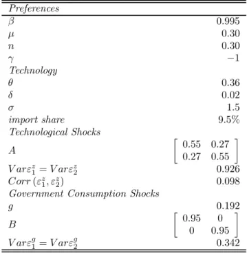
We choose the value of the variance of the shocks in order to reproduce the volatility of the GDP for the CEEC-10 found in empirical data. Table 4 presents a summary of the values for the benchmark parameters.
Table 4 - Benchm ark Calibration Param eters Preferences β 0.995 μ 0.30 n 0.30 γ −1 Technology θ 0.36 δ 0.02 σ 1.5 import share 9.5% Technological Shocks A ∙ 0.55 0.27 0.27 0.55 ¸ V arεz 1= V arεz2 0.926 Corr (εz 1, εz2) 0.098
Government Consumption Shocks
g 0.192 B ∙ 0.95 0 0 0.95 ¸ V arεg1= V arεg2 0.342
5
Results and Sensitivity
We simulate a model where the domestic economy is an aggregate of the ten transition countries at study (CEEC-10) and the foreign country is Germany, the biggest economy of the European Union and the one that has a significative amount of trade with these economies. The main purpose of the simulations of the model is to check if this model can replicate the S-Curve pattern found in the data for some of these countries.
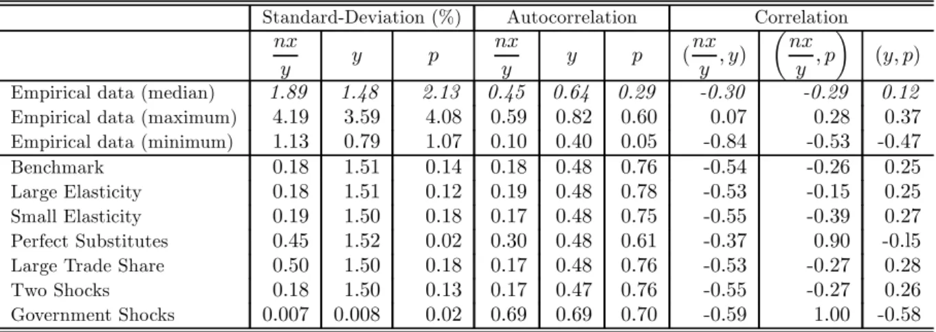
Empirical results for the CEEC-10 are replicated here again for ease of com-parison (in the first three rows we have the median values, the maximum val-ues, and the minimum values found in empirical data calculations). Theoretical benchmark results are presented in the fourth row of this table, while the re-maining rows present results for sensitivity analysis. Experiments made are described in the footnote of Table 5. Calibration for the two experiments with government shocks as well as parameter values for the benchmark simulation are described in Table 4 in the previous section.
Table 5 - Benchm ark and Sensitivity Analysis R esults
Standard-Deviation (%) Autocorrelation Correlation
nx y y p nx y y p ( nx y , y) µ nx y , p ¶ (y, p)
Empirical data (median) 1.89 1.48 2.13 0.45 0.64 0.29 -0.30 -0.29 0.12
Empirical data (maximum) 4.19 3.59 4.08 0.59 0.82 0.60 0.07 0.28 0.37
Empirical data (minimum) 1.13 0.79 1.07 0.10 0.40 0.05 -0.84 -0.53 -0.47
Benchmark 0.18 1.51 0.14 0.18 0.48 0.76 -0.54 -0.26 0.25
Large Elasticity 0.18 1.51 0.12 0.19 0.48 0.78 -0.53 -0.15 0.25
Small Elasticity 0.19 1.50 0.18 0.17 0.48 0.75 -0.55 -0.39 0.27
Perfect Substitutes 0.45 1.52 0.02 0.30 0.48 0.61 -0.37 0.90 -0.l5
Large Trade Share 0.50 1.50 0.18 0.17 0.48 0.76 -0.53 -0.27 0.28
Two Shocks 0.18 1.50 0.13 0.17 0.47 0.76 -0.55 -0.27 0.26
Government Shocks 0.007 0.008 0.02 0.69 0.69 0.70 -0.59 1.00 -0.58
Notes: Changes in the simulations were the following - large elasticity (σ = 2.5), small elasticity
(σ = 0.5), perfect substitutes (σ = 100),large trade share (import share = 20%).
Standard deviation for the trade balance and the terms of trade are consis-tently lower than the ones presented in the data. We made an experiment where we increased the import share for these countries, and another where domestic and imported goods were perfect substitutes and volatility for net exports sub-stantially increased. This feature also occurred in the article of Backus, Kehoe
and Kydland (1994), but in the developed countries analysed there, net exports and output are less volatile and terms of trade are more volatile than here. Output volatility is reasonably predicted by the model.
Since technology shocks are not much persistent, autocorrelation for these variables are not much persistent in the majority of the simulations, except for
the case of the terms of trade.2 However, it is worth noting that autocorrelations
obtained from the model are in line with empirical evidence from the group of countries in study.
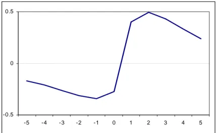
Correlations between these three variables in the benchmark economy ex-hibit a similar pattern observed in the data: correlations between net exports and output are negative, due to the strong volatility of investment that forces the economy to buy more imported goods after an increase in output due to a positive technology shock. This is also the reason why a S-Curve pattern ap-pears in the model in most simulations (a negative contemporaneous correlation between the terms of trade and net exports). Even with a positive technologi-cal shock and an increase in the terms of trade (in the real exchange rate) due to a decrease in domestic prices, an investment boom forces the trade balance into a deficit. This is a reasonable explanation, especially for transition coun-tries which are in much need of investment. Figure 3 shows this pattern for the benchmark economy. The same pattern is found in all simulations, except
“Gov-ernment Shocks” and “Perfect Substitutes”.3 Except for these two simulations,
the model seems to be quite robust to changes in the value of parameters.
2We experimented using the values of technological shocks used in Backus, Kehoe, and
Kydland (1994) and persistence increased. Results are available upon request.
-0.5 0 0.5
-5 -4 -3 -2 -1 0 1 2 3 4 5
Figure 3 - Cross-Correlation Function for the Benchmark Economy
Except for simulations ”perfect substitutes” and ”government shocks” con-temporaneous correlations between net exports and the terms of trade are neg-ative, as in the data (except for the case of Bulgaria and Hungary). These two mentioned simulations are the ones that don’t exhibit the S-Curve pattern, in-stead, they result in a tent-shaped curve, since the impact of investment in the trade balance is not so strong. After a positive technological shock, when domes-tic prices decreased and domesdomes-tic and imported goods are perfect substitutes, instead of running a deficit in the trade balance, the domestic economy runs a surplus, turning the correlation between the terms of trade and net exports positive. Positive government shocks usually make consumption and investment decrease, hence the country does not run a deficit in the trade balance. One example can be seen in Figure 4, where we exhibit the cross-correlation function between the terms of trade and the trade balance for simulation performed with government shocks only. Hence, if technology shocks are important to determine the existence of this pattern (and government shocks don’t), the knowledge of the nature of the shocks that constantly hit these economies is very important.
- 0 .2 0 0 .2 0 .4 0 .6 0 .8 1 - 5 - 4 - 3 - 2 - 1 0 1 2 3 4 5
Figure 4 - Cross-Correlations Function for Experiment Government Shocks
6
Conclusions
In this work we found empirical evidence of a S-Curve pattern for Slovenia, Czech Republic, Hungary, and also for an aggregate of the ten Central and Eastern European countries that recently joined the EU (CEEC-10). In the case of Lithuania, Poland, Romania, and Slovakia the pattern is weaker than in the mentioned countries but it stills prevails. Results for Bulgaria, Latvia, and Romania don’t show support for such pattern.
We then documented this property in the dynamic general equilibrium trade model of Backus, Kehoe and Kydland (1994) calibrated specifically for an econ-omy that represents the average economic conditions for the ten countries at study (CEEC-10). The model replicates well the observed pattern. The model is especially good in replicating autocorrelation patterns and cross-correlations between net exports and output, between net exports and terms of trade and between output and terms of trade.
Simulations performed to assess the robustness of the model found a very determinant role for technological shocks in the appearance of the S-Curve pat-tern, as in the work of Backus, Kehoe and Kydland (1994). Experiments with government shocks only and with perfect substitutes goods deliver a tent-shaped pattern instead of a S-Curve pattern.
In the center for the S-Curve explanation is the impact of technological shocks both in terms of trade (positive) and in the trade balance (negative, through investment). Since technological shocks are determinant in explaining the S-Curve pattern and transition countries seem to be experiencing some type of technological shocks, it is not likely that this pattern will fade away in the near future and hence it is important for economic policy to be aware of this phenomenon and its consequences for these countries in terms of real convergence and the timing of euro adoption.
References
[1] Armington, P. S. (1969), “A Theory of Demand for Products Distinguished by Place of Production”, IMF Staff Papers, March, 16(1), pp. 159-178. [2] Backus, D. K., Kehoe, P. J., and Kydland, F. E. (1994), “Dynamics of
the Trade Balance and the Terms of Trade: The J-Curve?”, American Economic Review, Vol. 84, Issue 1, March, 84-103.
[3] Cooley, T. F. (editor), (1995), Frontiers of Business Cycles Research, Princeton University Press.
[4] Bahmani-Oskooee, M., Kutan, A. (2008a), “Are Devaluations Contrac-tionary in Emerging Economies of Eastern Europe?”, Economic Change and Restructuring, Vol. 41, pp. 61-74.
[5] Bahmani-Oskooee, M., Kutan, A. (2008b), “The J-Curve in the Emerging Economies of Eastern Europe”, Applied Economics, Volume 41, Issue 20, pp. 2523-2532.
[6] Bahmani-Oskooee, M., Kutan, A., and Ratha, A. (2008c), “The S-Curve in Emerging Markets”, Comparative Economic Studies, Vol. 50, Issue 2, pp. 341-351.
[7] Égert, B., A., Morales-Zumaquero (2008), “Exchange Rate Regimes, For-eign Exchange Volatility and Export Performance in Central and Eastern Europe: Just Another Blur Project?”, Review of Development Economics, Vol. 12, Issue 3, August, pp. 577-593.
[8] Falk, M. (2008), “Determinants of the Trade Balance in Industrialized Countries”, FIW Research Report No. 13, June.
[9] Gollin, D. (2002), “Getting Income Shares Right”, Journal of Political Economy, Vol. 110, No.2, pp. 458-474.
[10] Herrman, S., Jochem, A. (2005), “Determinants of Current Account Devel-opments in the Central and East European Member States - Consequences for the Enlargement of the Euro Area”, Deutsche BundesBank Discussion
Paper No. 32.
[11] Junz, H. B., Rhomberg, R. R. (1973), “Price Competitiveness in Export Trade Among Industrial Countries”, American Economic Review, May (Pa-pers and Proceedings), Vol. 63 (2), pp. 412-418.
[12] Kemme, D., Teng, W. (2000), “Determinants of the Real Exchange Rate, Misalignments and Implications for Growth in Poland”, Economic Systems, Vol. 24, pp. 171-205.
[13] Magee, S. P. (1973), “Currency Contracts, Pass-Through, and Devalua-tion”, Brookings Papers on Economic Activity, No. 1, pp. 303-323.
[14] Meade, E. E. (1988), “Exchange Rates Adjustment, and the J-Curve”, Federal Reserve Bulletin, October, Vol. 74(10), pp. 633-644.
[15] Prescott, E. (1986), “Theory Ahead of Business-Cycle Measurement”, Carnegie-Rochester Conference on Public Policy Vol. 24, pp. 11-44. [16] Rahman, Jesmin (2008), “Current Account Developments in New Member
States of the European Union: Equilibrium, Excess, and EU-Phoria”, IMF Working Paper 08/92, April.
[17] Vanags, A., Bems, R. (2005), “Growth Acceleration in the Baltic States: What Can Growth Accounting Tell Us?”, Report by BICEPS.
[18] Whalley, J. (1985), Trade Liberalization Among Major Trading Areas, Cam-bridge, Massachusetts, MIT Press.
[19] Zienkowski, Leszek (2000), “Labor and Capital Productivity in Poland”, Central Statistics Office, Poland.
7
Appendix
Quarterly data used in Table 3 and Figures 1 and 2 were taken from the Eurostat electronic database NewCronos, from the Quarterly National Accounts. We have extracted GDP, export, and imports at current and constant 2000 prices for the widest period available for each country. The followings variables were then calculated:
• Real Output (y) - GDP at constant 2000 prices.
• Net Exports (nxy ) - Exports minus Imports divided by GDP at current
prices.
• Terms of Trade (p) - Implicit Price Deflator of Imports divided by the Implicit Price Deflator of Exports. The implicit deflators are obtained by dividing the current value of the variable by its constant value.
All variables are in logarithms except net exports as a percentage of GDP. H-P filter (with a parameter λ = 1600) was used to remove the trend and X-12 to remove seasonality, whenever data was not seasonally adjusted (as it was the case for Bulgaria, Czech Republic, Romania, and Slovakia). Time series for the ten transition countries are the following: Bulgaria - 1995:01-2008:01, Czech Republic, Hungary, Latvia, Lithuania, Poland, and Slovenia - 1995:012008:02, Estonia 1993:011995:012008:02, Romania 2000:011995:012008:02, and Slovakia -1992:01-2008:02.