Universidade do Minho Escola de Engenharia Departamento de Inform´atica
Alexandre Ventosa da Silva
A fully configurable virtual laboratory
of classical mechanics
Universidade do Minho
Escola de Engenharia Departamento de Inform´atica
Alexandre Ventosa da Silva
A fully configurable virtual laboratory
of classical mechanics
Master dissertation
Master Degree in Computer Science
Dissertation supervised by
Ant ´onio Ramires Fernandes
A B S T R A C T
Nowadays many mathematical applications allow the user to introduce its own equations in the system and also observe through different possibilities the desired results. Regard-ing physics, an extended range of virtual laboratories allow the user to accomplish virtual physics experiments. These virtual laboratories consist in predefined scenarios where the user can change the value of the physics variables and then visualise the changes accom-plished. Other virtual laboratories uses a physics engine allowing the user to create its own scenarios. However, the physical behaviour of the objects is hardcoded since it results strictly on the physics equations used internally by the physics engine.
This dissertation pretends to investigate how far and with what degree of scientific rigor it is possible to associate the idea of the user introducing its own equations with the idea of accomplishing virtual experiments of physics. As a proof of concept, this dissertation focus on a specific area of mechanics: the dynamic of rigid bodies. The result of this research is a virtual laboratory completely different relatively the others.
Our system has no knowledge about physics. Even the most general laws of physics such as the Newton’s second law are not known by the system. To the system, any equa-tion introduced is considered just as one more equaequa-tion without any particular meaning associated to it. The same happens for any physics entity. For example, if the gravitational acceleration is introduced by the user, to the system it is just another attribute of the world. Taking into account the dynamics of rigid bodies, an object can be identified as being, at any time, in one of three different states. These are: when a object is not in contact with any other, when an object collides with another object and they immediately separate, and when two objects remain in contact over time. The user must specify all the equations that drive each of these three states. Using its geometrical knowledge, the engine determines at any time in which state an object is. Also, the system provides all the relevant geometrical information. For instance, in a collision between two objects, the point and the two normals vectors of the collision are provided.
The graphical simulations reflects strictly on the equations introduced. Therefore, if the equations to solve a collision between two objects does not reflect the real underlying physics of the situation, it is possible that the objects simply ends-up penetrating each other. All the relevant numerical information about an experience can be processed through different forms. In fact, the user can request plots of variables, the graphical application of vectors on objects, and even the tracing of the variables at a specific event.
A C K N O W L E D G E M E N T
I would first like to thank my dissertation advisor Professor Doctor Ant ´onio Ramires Fer-nandes of the School of Engineering at University of Minho. The door of Prof. Ramires’s office was always open whenever I had a question about my research or the writing of the dissertation. I also consider that the weekly meetings we set ourselves were certainly a great help to the success of this research. He consistently allowed this dissertation to be my own work, but steered me in the right direction whenever he thought I needed it.
I also must express my very profound gratitude to my parents for providing me with unfailing support and continuous encouragement during those five years of study. This accomplishment would not have been possible without them. Thank you.
Alexandre
C O N T E N T S
1 i n t r o d u c t i o n 1
1.1 Description of the problem 1
1.2 Work motivation 2
1.3 Structuring of the document 2
2 s tat e o f t h e a r t 4
2.1 Physion 5
2.2 VPLab 7
2.3 Interactive Physics 8
2.4 Phet Interactive Simulations 12
2.5 My Physics Lab 13
2.6 Conclusion 15
3 t h e v i r t ua f i z pa r a d i g m 16
3.1 Overview of the system 16
3.2 The concept of context 17
3.3 The engine behind VirtuaFiz 21
4 t h e v i r t ua f i z s i m u l at i o n s p e c i f i c at i o n 26
4.1 The VFLang programming language 26
4.2 The specification of two simple simulations 29
5 a d va n c e d c o n t e x t s w i t h r e a l p h y s i c s 42
5.1 The free fall context 43
5.2 The collision context 47
5.2.1 Collision between a dynamic and a static object 51
5.2.2 Collision between two dynamic objects 68
5.3 The contact context 74
6 t h e v i r t ua f i z e n v i r o n m e n t 79
6.1 Tracing of variables 79
6.2 Visualisation of trajectories and vectors 80
6.3 Visualisation of plots 83
6.4 The VFLang interpreter 85
7 c o n c l u s i o n 88
7.1 Future Work 88
Appendices 90
a s o m e u s e f u l v f l a n g nat i v e f u n c t i o n s 91
L I S T O F F I G U R E S
Figure 1 A simple Physion scenario composed by the predefined container, a
spring and also a sphere 6
Figure 2 An example of a plot generated by Physion relative to a attribute of an object that integrates an experience. 6
Figure 3 Gadget created in Physion capable of climbing stairs 7
Figure 4 Main window of experience ”Explaining Electricity” that is part of the suite of experiences provided by VPLab 9
Figure 5 From left to right, the physics theory and the instructions necessary to accomplish properly experience ”Explaining Electricity” 9
Figure 6 A possible scenario in Interactive Physics composed by several rigid bodies to represent a scale and two weights 10
Figure 7 Final configuration of the scenario described in figure 6. The anchors and rotation points required for a correct execution of the experiment
were also specified 11
Figure 8 ”State of Matter: Basics” experience interface, included in the exper-iments provided by Phet Interactive Simulations 13
Figure 9 Single Pendulum experience interface, included in the experiments
provided by My Physics Lab 14
Figure 10 Example of a plot generated by My Physics Lab 14
Figure 11 An example of a parabola trajectory described by the sphere during its free fall motion according to equation 5 18
Figure 12 The mathematical collision response calculation according to
equa-tion 6 19
Figure 13 A simulation of a cube colliding multiple times with a ramp until it ends up sliding on its surface 21
Figure 14 A VirtuaFiz simulation containing 7 objects distributed in two differ-ent contact context instances 22
Figure 15 Due to its specific initial position and initial velocity, each cuboid is in collision with the other three 23
Figure 16 A possible outcome of the simulation involving the sphere and the
cuboid. 31
List of Figures v
Figure 17 A possible outcome of the simulation involving the sphere and the cuboid. The sphere penetrates the cuboid since the collision response
specified is empty. 35
Figure 18 A possible collision between two spheres and the respective response according to the environment described 39
Figure 19 Changes in position and orientation suffered by the cuboid during the first free fall context application 45
Figure 20 The restitution coefficient for some pair of materials 48
Figure 21 The static and dynamic friction coefficient for some pair of
materi-als 49
Figure 22 Without a friction force acting on the sphere at the time of the colli-sion, the angular velocity of the sphere remains unchanged 50
Figure 23 The friction force acting on the sphere at the time of the collision, induces a change in the angular velocity of the sphere 50
Figure 24 The torque depends on the orientation of the objects at the time of
the collision 53
Figure 25 The world system coordinates (left) and the collision system
coordi-nates (right) 57
Figure 26 A scenario composed by two different contact context instances whose complexity is supported by the contact context built in this
sec-tion 75
Figure 27 The forces and its components involved in a contact between two
objects 76
Figure 28 The interface displayed by VirtuaFiz containing all the relevant in-formation about a specific event 81
Figure 29 A possibility of trajectories followed by the objects in a simulation 82
Figure 30 The visualisation of vectors applied on objects at the time of an
event 82
Figure 31 A plot showing coordinate z of a dynamic sphere changing over time in a simulation composed by the sphere and a static cuboid 84
Figure 32 A plot showing the variation over time of the normal reaction force’s norm of an object in a simulation composed by 3 dynamic and 1
static cuboids 84
Figure 33 The calculation of the collision response between two spheres using
1
I N T R O D U C T I O NThe main theme of this dissertation is virtual physics simulation. While there are many readily available 2D/3D simulations, these are usually hand crafted for a specific simula-tion. Furthermore, the user is only allowed to play with the simulation’s parameters, the underlying physics is most of the time hidden from the user.
We propose a different approach to build these simulations, which we could categorise as ”do it yourself physics”. In our proposal the user gets full control, not only of the parameters but also of the underlying physics, i.e., the equations themselves. In fact, before our system can simulate any physical phenomena the user has to introduce the equations that govern the specific phenomena.
In this chapter an initial approach to the problem is presented. The reasons justifying the need for this investigation are founded. An overview about the objectives we intend to achieve with this investigation is also presented.
1.1 d e s c r i p t i o n o f t h e p r o b l e m
The lack of adequate and necessary laboratory material in many educational facilities, or allowing a student, in a home-work context, to learn physics through a virtual test environ-ment, has led to the development of the most varied tools that reproduce through virtual laboratories different physics experiments.
The main objective of these virtual laboratories of Physics is to provide the student with new knowledge in the fields of Physics that he is studying. In fact, in physics classes, the focus given to the laboratory is central. Much more than a place at the back of the classroom, it is in the laboratory that physics students ”do” physics. It is in this test environment that the students start out the typical activities of scientists - questioning themselves, applying procedures, collecting data, analysing data, answering questions from their colleagues and teachers, or thinking about new issues and possible scenarios to explore.
Currently, there are several software solutions that allow the student to recreate in a virtual environment certain Classical Physics experiments. These platforms offer a wide range of experiences covering the various areas of physics: hydrodynamics, hydrostatics,
1.2. Work motivation 2 kinematics, dynamics, electromagnetism, among others. This ”supply” variety brings with it the disadvantage that, in one experiment, the user can only change a small set of pa-rameters. It is also known that these experiments are generally defined based on a set of predefined scenarios, and it is not possible to change them. These characteristics allow to visualise the result of a certain test configuration and the variation, over time, of the val-ues of the relevant physical variables which come within the context of the experiment. In short, the physics is built-in in these simulations, and the student is only allowed to set parameters. Most of the time the student does not even have access to the equations used in the simulation.
1.2 w o r k m o t i vat i o n
The approach taken by these pedagogical tools does not allow the student to develop an in-depth knowledge and skills about ”why” or ”how” a particular physical phenomenon occurs. In fact, we believe that only by knowing the underlying Physics that sustains a particular physical phenomenon, is it possible to fully understand the behaviours that occur in an experience and apply the knowledge in other experiences or in real cases.
This research intends to create a tool that exploits a new paradigm in the teaching of Physics through virtual laboratories. In this sense, we propose a generic engine that has no knowledge of physics. It becomes the user responsibility to introduce all the mathemat-ical formulas and equations that support a certain physmathemat-ical phenomenon that one wants to study. Even the most general laws of physics, such as, for example, Newton’s second law, would not be known by the system a priori. This drastic approach may at first seem unnecessary and would complicate the work of potential users. However, as previously stated, we believe that only with a complete idea of the formulas and equations that under-lie a physical occurrence, is it possible to properly extract and apply the concepts outside the restricted and closed context that characterise virtual experiences. As will be shown, to properly animate these equations the engine only needs to have built-in geometry knowl-edge. 3D simulations are provided by the engine based on the geometry it knows, and the equations the user inputs. As a proof of concept this dissertation focus on a specific subarea of classical mechanics: the dynamics of rigid bodies.
1.3 s t r u c t u r i n g o f t h e d o c u m e n t
In addition to the present chapter, this dissertation is structured in 5 chapters. A State of the art is presented in chapter2. In chapter3our approach to the problem is presented. Chapter 4covers how in practise an experience can be defined following the approach described in
1.3. Structuring of the document 3 we cover the steps about how the actual physics equations that drive the mechanics of rigid bodies can be specified in our tool. Using the graphical interface of the developed software, in chapter 6, we present various features of the tool related to how the numerical
data inherent to a specific experience can be processed and visualised through various possibilities. Finally, a conclusion about all the work developed is presented in chapter7.
2
S TAT E O F T H E A R TNowadays there are many programs dedicated to the teaching of physics that allow to recreate, in a virtual environment, experiments of physics such Central Connecticut State University, Neumann, Nunn, Duncan, Virtual Science Ltd, Xanthopoulos, Design Simu-lation Tecnologies, University of Colorado Boulder, among many others. The degree of freedom and configuration of the scenario and the bodies composing an experience, as well as the possibility of specifying a concrete response to certain events, such as a collision between two bodies, differs among solutions. In fact, all the applications analysed in the context of this dissertation implement the response to this type of events in a ”hardcoded” way. It means that it is not possible for the user to specify the behaviour he would like to observe, or to really understand what physical foundations and mathematical equations are behind the observed physical phenomenon. The bodies or particles of an experiment possess a closed and predefined set of attributes. Each attribute corresponds to a certain physical variable which is necessary for the context of the experience. For example, in classical mechanics, one of these object attributes can be the mass, or the coefficient of restitution.
The possibility and also the way it is possible to reach conclusions about the data related to the events of the experience, for example, by providing plots of the physical variables, also differs greatly from one tool to another.
Given the wide range of software applications associated with this problem, it would not be possible to present in this chapter the characteristics and functionalities of each one individually. Thus, a set of the applications representing a relevant sample of the solutions is described below. In selecting the applications that would integrate this sample, care was taken to choose those whose functionalities and characteristics differ from the rest so that we present a broad idea of what is currently available and what functionalities can be extracted from this kind of tools. Also, in the case of solutions that offer similar functionality to the users, we choose the ones that appear to be more popular and used by a larger number of people.
In sections 2.1, 2.2, 2.3, 2.4 and2.5, the main features and functionality of Physion
Xan-thopoulos, VPLabNunn, Interactive PhysicsDesign Simulation Tecnologies, Phet Interactive
2.1. Physion 5 SimulationsUniversity of Colorado Boulder and My Physics LabNeumann are presented, respectively.
2.1 p h y s i o n
Physion is a computer program created by Dimitris Xanthopoulos in 2010 that allows the simulation of physics, in a two-dimensional way, associated with the mechanics of rigid bodies. This program can be used to easily create a wide range of interactive physics simulations and educational experiences. The application uses a physics engine called Box2DCatto to detect and resolve collisions between bodies present in a given scenario.
Using the tools provided by the application, the user can create several physical objects, such as circles, polygons, ropes, pulleys, among others. Each rigid body present in an experiment can be a static or dynamic body. A static body has a fixed initial position assigned and will not move under any circumstances during all the time of the experiment. A dynamic body is a free body not subjected to any restriction of movement, so forces acting on it can induce a change in its velocity. The application provides an attribute editor. It is thus possible to specify for each body its density, its position relative to the two dimensions of the scene, its restitution coefficient, the type of body (rigid or dynamic), its initial linear and angular velocity, among others. The user has to restrict himself to this finite series of predefined attributes because it is not possible for the user to declare new ones.
Through the window containing the scene properties, the user can specify the numerical value to be assigned to the gravitational acceleration in the two orthogonal axes or the frequency at which the scene is recalculated. The scene and its visualisation is configurable, therefore it is possible to change the background colour or the attributes related to the camera.
By default, a newly created scenario already contains three rectangles that form a static container. To static bodies is applied a brick texture to emphasise the idea that it is a fixed element of the scenario. Figure1represents a circle and a spring that connects the circle and
the predefined left vertical rectangle. Accessing the spring attributes editor, it is possible to change the proper attributes of a spring, such as the constant k of the spring. The constant k corresponds to the elasticity of the spring. Physion uses Hooke’s law to calculate the force exerted by a spring:
F = −k∗x (1)
The greater the displacement x in relation to the steady state of the spring and the greater constant k, the greater is the force exerted by the spring. Hooke’s law is used internally by the system and the user can not modify the law or specify its own equation.
2.1. Physion 6
Figure 1.: A simple Physion scenario composed by the predefined container, a spring and also a sphere
Figure 2.: An example of a plot generated by Physion relative to a attribute of an object that inte-grates an experience.
By changing the restitution coefficient of the circle, the spring constant, or the circle density, viewing the new graphical simulation associated with the new configuration allows us to understand quickly the effects induced by the changes made. For instance, for a density equal to 1, the circle does not touch the horizontal rectangle due to the force exerted by the spring, whereas for a density of 100, the spring can not counteract the gravitational force exerted on the circle, so it ends up quickly and inevitably colliding with the horizontal rectangle.
Physion allows the creation of plots. However, just to observe how the acceleration and speed of a particular body varies over time of experience. Figure 2 represents the plot
obtained for the speed of a circle with a given initial position and radius, relative to the scenario previously described and for the concrete case of its density to be equal to 100.
One advantage of Physion is the ability for the user to enter their scripts written in javaScript. It is therefore possible for the user to specify through scripts some kind of behaviour that could not be possible to be specified by the conventional tools provided to the user. However, the script cannot be used to change the underlying physics of an
2.2. VPLab 7
Figure 3.: Gadget created in Physion capable of climbing stairs
experience. All the physics equations are hardcoded in the physics engine used by the application. With that said, the degree of configurability remains limited and the scripts are mainly used for artistic purposes, such as for changing the colour of a spring according to its deformation at a given moment, or for specifying ”invisible” forces, i.e., forces that act at distance, such as the gravitational force generated by a very large mass, and that acts in each of the bodies that is in its vicinity.
By combining conveniently the various primitives offered by the application it is possible to create interesting and relatively complex experiences. Figure3illustrates an experiment
created with Physion where it is possible to observe a robot, composed of several springs and rectangles articulated together, that is able to climb the steps of a staircase.
2.2 v p l a b
Virtual Physical Laboratory (VPLab) is a suite of more than three hundred small interactive physics simulations. It is a paid tool and only available for Windows. However, it is possible to have access to a demonstration of the tool through seven executables, corresponding to seven different experiments. John Nunn began to develop this tool in the year 2000, and today is perhaps the most well-known and used tool for teaching of Physics in high schools around the globe. The tool is approved by the National Physical Laboratory, the UK’s national weights and measures laboratory, based at Bushy Park in Teddington.
In all simulations provided by VPLab, a level of difficulty is assigned so one can see if the student’s age corresponds to the expected age and its experience. ”Basic” targets 12-16 year old’s, while an ”Advanced Level” experience is expected to be solved by a student between the ages of 17 and 19.
2.3. Interactive Physics 8 The three hundred and thirty-four experiments provided by the software are grouped into thirty-one different categories, corresponding to the different areas of research covered by Physics. In this sense, the tool makes it possible to perform and assimilate knowledge about astronomy, or from a completely different area such as Electromagnetism or Fluid Mechanics.
An experiment is represented by a predefined scenario. Figure 4 illustrates the
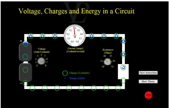
corre-sponding graphical interface of an experiment included in the set of free samples. This experiment aims to present and explain the basic concepts of electricity. As it can be seen, the experiment is composed of a small electric circuit, consisting on a battery, an ammeter and a resistance. The user can learn about the theoretical concepts related to the experience or about the functionalities and the purpose intended for it. Figure5shows the two views
presented to the user, the one on the left corresponds to the instructions, while the one on the right presents the theory.
By playing around with the two buttons associated with the battery voltage and the value of the resistance, the user sees interesting things happening. Thus, an increase in the voltage of the battery, causes an increase in the energy transported by each electric charge. Also, the charges begin to move faster. Relatively to the resistance, an increase in its value causes the opposite effect, that is, the charges move more slowly. In fact, there is a decrease in the value of the current (due to a greater dissipation of energy in the resistance). These phenomena are due to Ohm’s law:
V =R∗I (2)
The graphical representation of the ammeter is an added value in the context of the experiment, since it allows to confirm the Ohm’s Law by observing what the law predicts when changing the values of the voltage and the resistance.
All of the experiences provided by VPLab follow the same philosophy. It is possible to have access to a window explaining the theory behind the experiment, as well as another window explaining in detail what it is possible for the user to change (physical variables) and what it is expected to happen from the changes made. The degree of configuration by the user is limited and is essentially based on the change of the numerical value associated with a particular physical variable.
2.3 i n t e r a c t i v e p h y s i c s
Interactive Physics is an application developed by Design Simulation Technologies that consists of a virtual environment in which it is possible for the user to set up their own test scenario through the tools provided by the program. There is a large community composed mostly of teachers who contribute to the creation of new experiences. Therefore, there is
2.3. Interactive Physics 9
Figure 4.: Main window of experience ”Explaining Electricity” that is part of the suite of experiences provided by VPLab
Figure 5.: From left to right, the physics theory and the instructions necessary to accomplish prop-erly experience ”Explaining Electricity”
2.3. Interactive Physics 10
Figure 6.: A possible scenario in Interactive Physics composed by several rigid bodies to represent a scale and two weights
the possibility of anyone submitting their experience through the official website of the tool and, if approved, the experience will be available to the community. Using this tool it is possible to perform physics experiments that fall into the topics of collisions, electrostatics, gravitation, friction, kinematics, oscillations, projectiles, among others. The simulations are performed in a two dimensional environment.
The program allows the user to include a wide range of possibilities for the objects to integrate in the test environment. For instance, it is possible to create objects by drawing circles, blocks or any other type of polygons. It is also possible to create more complex objects such as ropes, springs, pulleys, among others. The application allows to simulate contact between bodies, as well as collisions or the frictional forces involved. Several fam-ilies of forces are predefined. Setting their numerical value, allows the user to quickly observe their effect on the object. For example, the air resistance force induces a change on the velocity of the object. Interactive Physics allows the user to create plots. The possibili-ties to create different kind of plots are many. It is possible to visualise how the position, velocity and acceleration (linear or angular), as well as their momentum (linear or angular), vary over time. The application also allows the drawing of plots to observe the variation of the total force that acts in a body, as well as the torque, the gravitational force, electrostatic or the air resistance. The application is concerned with the user experience. It is possible to specify that a sound must be emitted for the instants in which two bodies collide. Another possibility of the application is to study the properties of the sound wave. For instance, the application allows the user to measure and listen to sounds affects to a certain volume and frequency.
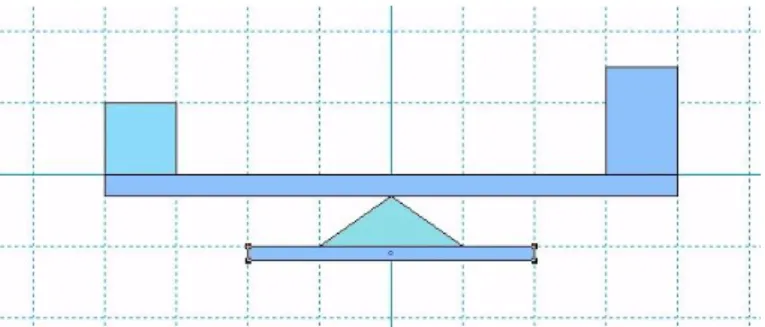
Figure6represents the configuration of a scenario, where several rectangles and a triangle
were drawn. These objects are meant to represent a scale and two weights. If the simulation were to proceed immediately, these objects would all fall apart in disorder due to the action of the system pre-defined gravitational force. The pallet with the tools provided by the application allows, for example, by means of anchors and fixed points, that is possible to fix an object in the space, or to specify a point of rotation, respectively.
2.3. Interactive Physics 11
Figure 7.: Final configuration of the scenario described in figure6. The anchors and rotation points
required for a correct execution of the experiment were also specified
Interactive Physics also allows the design of vectors acting at some point in a body to represent the actual value of a physical entity. It is also possible to texture a given object to make the simulation visually more appealing.
After adding the necessary anchors and rotation points to represent the intended be-haviour of a scale, the user is able to observe a functional scale. Figure 7 represents the
result obtained, for an instant of time equal to 2 seconds. It is possible to observe that the two weights present in the scale were textured with pictures of a weight and a hand. Also, the two vectors were drawn in red. They are applied in each weight, representing the respective gravitational force, according to its direction and intensity. For the design of the forces, it was further specified that it was intended to visualise the norm of the vector, expressed in Newton in this case, since it is a force.
It is also possible to observe in figure7that two sliders were introduced in the experience.
They allow to change the position of each weight placed in the scale. As intended, the side which the scale inclines depends on the chosen configuration of positions.
The physical phenomenon to be studied in this experiment is called torque. For the scale to be in equilibrium it is necessary that the total torque is 0, with the following equation being verified:
F1∗d1 =F2∗d2 (3)
This means that the normal force acting on one side of the scale F1 multiplied by the distance from its point of actuation to the centre d1 (axis of rotation of the lever) is equal
2.4. Phet Interactive Simulations 12 to the normal force acting on the other side F2 multiplied by the distance from its point of actuation to the centre d2.
As we realised with the experience pictured in figure7, the user can easily create a scale
and place some weights on it and observe which side the scale tilts due to the torque. However, not even the notion of torque, and what are the entities involved in its calculation just as described in this section are mentioned in Interactive Physics.
2.4 p h e t i n t e r a c t i v e s i m u l at i o n s
Phet Interactive Simulations consists of a set of physics experiments, available free of charge and elaborated by the University of Colorado Boulder. At the Phet Interactive Simulations website the user can find experiences about the most varied topics of physics, biology, chem-istry, among other scientific areas. Experiments run directly on the user’s web browser.
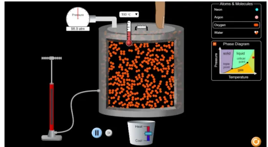
Figure8shows a view of the window presented to the user for the ”State of Matter:
Ba-sics” experiment. This experiment is included, along with fourteen other experiments, in the section of heat and thermodynamics. The experience intends to introduce the student to the basic concepts of pressure and temperature and how these vary in the context of a thermally insulated container with variable volume. The user is presented with an ex-planatory diagram regarding the theoretical concepts that are intended to be studied in this experiment. The user can interact with the scenario and observe the result the introduced variations induced. In that sense, through a pump, it is possible to increase the number of corpuscles present in the vessel. It is also possible to heat or cool the vessel, to change the nature of the molecule to be studied, or to increase or decrease the volume of the vessel. The pressure and temperature indicators allow visualising the numerical value associated with these two physical variables. This experience sensitises the student about the physical concepts in action through a qualitative analysis of the events. However, it is more compli-cated to extract more in-depth knowledge since it is not possible to rigorously quantify, for example, the energy supplied or withdrawn to the vessel by the heater and cooler. It is also not possible to accurately conclude the number of atoms or molecules present in the vessel, and the concrete result induced by the action of pumping on the variation of the number of particles.
In fact, the experiences of the Phet interactive simulations suite follow the characteristics of the experience described above. The goal of this type of software solution is to introduce, through appealing graphics and a modern interface, concepts related to physics present in a given context. The degree of customisation of the scenarios, as well as how the data inherent to the experience, can be scientifically processed, for example through graphics, is quite limited.
2.5. My Physics Lab 13
Figure 8.: ”State of Matter: Basics” experience interface, included in the experiments provided by Phet Interactive Simulations
2.5 m y p h y s i c s l a b
My Physics Lab is a website created by Erik Neumann in 2001 containing physics exper-iments. Over time, new experiences have been added by the author. Currently, the site makes available fifty-three experiments to be performed directly in the browser. All the experiments are access free. These experiments intend to present the concepts related to classical mechanics. Special emphasis is given to the mechanics of springs, pendulums, roller coasters and the dynamics of rigid bodies.
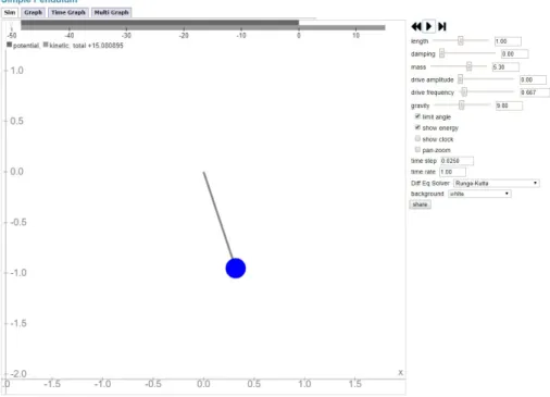
Figure9shows the ”Single Pendulum” experiment environment. The experiment allows
to change an advanced set of predefined parameters, such as the pendulum chord size, energy dissipation factor, pendulum mass, gravitational acceleration, among others. There are many possibilities for processing and presenting data. For instance, it is possible to request plots, relating any physical variables treated in the context of the experiment. For the concrete experiment of ”Single Pendulum”, it is then possible to relate, along with time, the following physical variables associated with the pendulum: angle, angular velocity, angular acceleration, kinetic energy, gravitational potential energy and total energy. The figure10illustrates the plot obtained for the variation of the kinetic energy of the pendulum
as a function of time ranging from 0 to 14. The plot follows the simulation specifications for the numerical values assigned to the parameters shown in the figure9.
The user has access to a theoretical context where the physics that underlies the move-ment described by the pendulum is explained, as well as the energies that come into play. It is also presented information to the user about how it is possible to solve numerically the differential equation associated with the pendulum movement. The various numerical
2.5. My Physics Lab 14
Figure 9.: Single Pendulum experience interface, included in the experiments provided by My Physics Lab
2.6. Conclusion 15 resolution hypotheses are explained. The user can select the desired solver as well as the integration step. The differential equation presented by My Physics Lab that translates the pendulum motion subject only to the action of the gravitational force is:
d2θ dt2 +
g
Lsin(θ) =0 (4)
where g is the acceleration of gravity, L the length of the wire and θ the angle described by the pendulum relatively to the vertical axis.
Most of the experiments provided by My Physics Lab follow the philosophy behind the Single Pendulum experience. Thus, regarding the possibilities of configuration, the user can vary the numerical value of a wide range of parameters, relate in a graph two physical variables of the experiment. Two other pedagogical peculiarities associated with this platform are the fact that one has access to the physical theory of the experience as well as information regarding the numerical resolution of the problem, starting from the physical equations presented in the section of the physical theory.
2.6 c o n c l u s i o n
From the applications we covered in this chapter, we understand that two families of physics virtual laboratories are easily identified. On one side, applications such as 2.2
consist of predefined scenarios without the possibility of creating new objects to partici-pate in the experiment. In this family of applications, the user has the freedom to change the value of some predefined physics entities associated to the experience and observe the induced results. On the other side, applications such as 2.1 allows the user to specify all
the objects wanted to be part of the experiment. This is made possible by the existence of a physics engine. However, we saw that the physics equations used by the engines are hardcoded and the user has not the possibility to change or even visualise the equations. Therefore, any desired change to the underlying physics would only be possible to be done by the authors of the applications. From a pedagogical point of view, another disadvantage is the fact that since the student has no access to the equations used, it is difficult for him to associate the visualisation of a specific physics phenomena with its respective mathematical description.
3
T H E V I R T U A F I Z PA R A D I G MThis chapter presents the paradigm and the philosophy behind the developed tool. Section
3.1presents an overview of the system and what it intends to accomplish. In section3.2the
reasons that led us to create a new and innovative concept in physics virtual laboratories are presented through theoretical examples. We name this concept Context and its formal definition is also presented in this section. Finally, in section3.3we explore some
particu-larities of the engine behind VirtuaFiz. It is also in this section that a differentiation is made about which steps are user or system responsibility during the whole process of preparing and then performing a simulation.
3.1 ov e r v i e w o f t h e s y s t e m
As detailed in chapter 2, the physics virtual laboratories that exist today are essentially
tools that allow to observe a certain physical phenomenon by adjusting the values of a predefined set of parameters ”hardcoded” in the system.
While in VirtuaFiz the visualisation of physical experiments, and parameter adjustment, is also possible, the main emphasis is not on the visualisation of pre-built experiments, but rather to allow the creation of new experiments through the introduction of the equations that rule the experiment.
VirtuaFiz takes the idea of the specification of the physics by the user to an upper level. In fact, the system does not have any knowledge about physics. Every physical phenomena observed results strictly of the equations that the user specifies. Therefore, if some equation introduced in the system does not reflect the physical behaviour that would be observed in the real world, the observed result in VirtuaFiz will look unrealistic. This feature makes the major difference between previous solutions and VirtuaFiz. In fact, this approach can be seen as a new paradigm of specifying physics in virtual laboratories. Due to its nature, VirtuaFiz is especially geared towards the teaching of physics to the level teached in high school and also in some introductory subjects of classical mechanics in a college degree.
Regarding the test environment, the tool is quite similar in relation to the others. In fact, the system is able create graphical simulations with one or more objects evolving in a
3.2. The concept of context 17 world and then observe the physical interactions that happen between objects. From these interactions, changes in the trajectories and behaviour of the objects may occur. Generally in virtual laboratories, a three dimensional orthogonal referential is used to represent a specific position in the world. Also, the world space has no boundaries and is conceptu-ally infinite. The world possess some attributes (time, for example). With respect to the objects, they possess attributes (position and mass, for example) and have a physical and geometrical type. The geometrical type of an object is its shape while its physical type can be static or dynamic. Contrary to a dynamic object, a static object will not see any of its attributes updated during a simulation. VirtuaFiz follows globally the same conventions described above to specify the world or an object. However, contrary to the others tools, all the attributes are defined by the user. For the system they have no particular meaning (contrary to the gravitational acceleration or the restitution coefficient attributes we can see in many labs, for example). The meaning of an attribute is the one the user intends to give him conceptually. Exceptions are the predefined world attribute time and the predefined geometric objects attributes position, size and orientation.
3.2 t h e c o n c e p t o f c o n t e x t
As we stated in section 3.1, VirtuaFiz intends to follow a different approach about how a
simulation is specified and what the system ”knows” about physics. Since according to the new paradigm we identified, all the physics is specified by the user, to understand the necessity of the new concept we introduce in this section nothing better than look at two simple examples and remember the physics equations we all used in high school to describe the situations encountered.
Let’s start with a simple example of a sphere, starting from a position p0 at time t0, and evolving in space where a constant gravitational field, with acceleration a, is acting. Consider also that the sphere has some initial linear velocity v0. For a given moment t, the position p of the sphere can be known using the following kinematic equation:
p= p0+v0(t−t0) + 1
2a(t−t0)
2 (5)
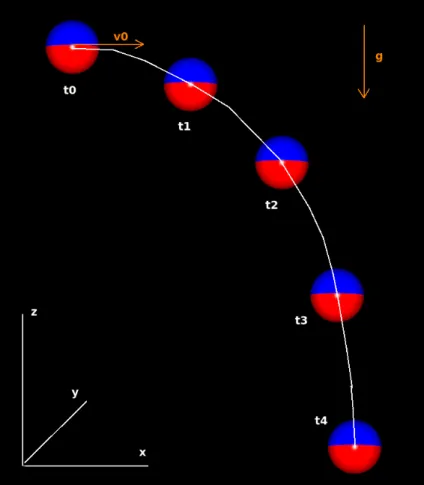
Figure11shows a possible parabola trajectory followed by the sphere during its free fall
motion as described by equation5. The initial velocity and gravitational acceleration vectors
have the direction of the semi positive axis X and the negative semi negative Z, respectively. t0, t1, t2, t3 and t4 represented in figure 11 are four equidistant time moments. As we
can see from the figure, the fall delta made by sphere between two successive moments increases continuously from one pair to the next. This is due to the square power associated with the expression(t−t0)in equation5.
3.2. The concept of context 18
Figure 11.: An example of a parabola trajectory described by the sphere during its free fall motion according to equation5
3.2. The concept of context 19
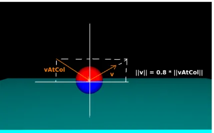
Figure 12.: The mathematical collision response calculation according to equation6
Equation5describes the behaviour of a sphere in free fall. Now, let’s assume that
eventu-ally the sphere, during its fall, collides with the ground, represented by a flat cuboid. Surely equation5above cannot be used to solve the collision response between the two objects. In
fact, specific equations are needed to solve this particular problem. Let’s just assume the cuboid is static, horizontally oriented, and large enough so that the sphere can only col-lides with its upper horizontal face. Also, let’s consider at the moment of the collision, the sphere velocity is mathematically reflected but due to some loss of energy, it also reduced by a factor of 20%. The simple equation below can be used to calculate the velocity vector v of the sphere immediately after the collision, assuming axis Z is the vertical axis:
v=0.8∗ (vAtCol.x, vAtCol.y,−vAtCol.z) (6) where vAtCol is the sphere velocity at the moment of the collision and the .x, .y and .z annotations represent the first, second and third components of a vector, respectively.
Figure 12 shows what happens to the sphere velocity when it collides with the cuboid
according to all the conditions stated earlier.
This approach and all restrictions mentioned above make the simulation very limited about the behaviours that can observed and also physically unrealistic. In fact, the physics behind collision response are very complex involving many mathematical and physical concepts. The physics behind the collision response between two bodies independently of their shape or even their orientation in space at the moment of the collision are introduced in chapter 5. For now, let’s just keep with the restrictions stated earlier. They keep the
example simple and keep us from loosing the focus of what this section is about.
Through the two situations presented, we understand that an object in free fall and an object colliding with another one, introduces necessarily different scenarios, requiring
dif-3.2. The concept of context 20 ferent sets of equations for each particular scenario. In both situations described, the un-derlying physics are also different. For these reasons, VirtuaFiz introduces the notion of physics contexts used to differentiate into specific environments the different physical be-haviours the user intends to observe.
Relatively to the specificities of a context in VirtuaFiz, a context is a specific environment where a given object evolves. At any time during a simulation, every object has only one specific context applied on it. Besides object and world attributes, context attributes can be defined within a context. One instance of these context attributes is made for every object involved in the context. The scope of these attributes is limited to the context. This means when an object leaves a specific context, the value of the attributes is lost and a later return to the same context will reset their values. On the other hand, an object attribute must be used when its meaning and value transcends a specific context application.
A context is composed by a set of functions introduced by the user. During a simulation, the attributes of each object, as well as the world and context attributes are constantly being updated using the functions of the context where the object evolves. The functions tells the physical behaviour to be observed in a particular situation. This is made possible by functions whose name is the name of an object, world or context attribute. The number of objects involved simultaneously in a specific context instance depends on the type of the context. A context have one of the three following types: free fall, collision and contact.
Free fall contexts must be defined to describe the physical behaviour wanted when an object is not in physical contact with any other object. Since in a free fall context an object does not interact with another and can maintain this behaviour for a continuous time, a free fall context instance is applied to a single object and is applied continuously during a sequence of frames.
Collision contexts must be defined to describe the physical behaviour wanted when two specifics objects collides. In the real world, when two objects collide, depending on its materials, the objects stay in contact during a more or less important time interval. However, in general this time interval tends to be relatively small so in practise we can consider it to be zero. Therefore, contrary to a free fall context, a collision context application is not continuous and occurs only one time within a frame. One could argue that this reasoning is not valid in the presence of a non elastic collision when the objects are in contact for a longer time. However, if the user builds a collision context using real physics, by defining, among others, the restitution coefficient and all the necessary physical equations, the behaviour of the objects after the collision will be just as it would be observed in real life.
Let’s observe figure 13 to understand the necessity of having a third type of context in
VirtuaFiz. In the real world, every time a cube collides with a ramp, a very strong force (much more than the gravitational force acting on the cube) acts during a small interval of time, on the cube. The result of a force acting during a certain amount of time is called
3.3. The engine behind VirtuaFiz 21
Figure 13.: A simulation of a cube colliding multiple times with a ramp until it ends up sliding on its surface
an impulse. The effect of the impulse on the cube is to generate a change in its velocity. Overtime, after multiples collisions and energy losses, the impulse acting on the cube is no longer effective to induce a change in the velocity of the cube that would fight the gravitational force and separate it from the ramp. In this case, regarding the collision normal axis, the normal reaction and gravitational forces ends up cancelling each other continuously over time, making the cube remaining in a prolonged contact with ramp.
In order to cope with the possibility that the user wishes to specify real physics in its con-texts by following, for example, an impulse approach for collisions and a force approach for prolonged contacts, VirtuaFiz allows the definition of Contact Contexts. Therefore, when a collision context is no longer effective, the system automatically switches to a contact context. A collision context is no longer effective when after its application the objects are not able to separate or end up penetrating each other. This is what would happen in the simulation pictured in figure13if there was not a VirtuaFiz contact context defined for this
simulation. Just as a free fall context, a contact context is applied continuously. Contrary to a free fall context instance and a collision context instance that always contain one and two objects, respectively, a contact context instance can contain an arbitrary number of objects. Figure 14 shows two different contact context instances that are simultaneously applied
over time. In the figure, the instance pictured on the left contains 3 objects while the one on the right contains 4 objects.
3.3 t h e e n g i n e b e h i n d v i r t ua f i z
Before we explain some particularities of the system, it is important to detail the philosophy followed by VirtuaFiz. As previously stated the system has no knowledge about physics.
3.3. The engine behind VirtuaFiz 22
Figure 14.: A VirtuaFiz simulation containing 7 objects distributed in two different contact context instances
However, the engine has knowledge about the geometry involved in a simulation, and uses that knowledge to determine which context to apply at any particular time to each particular object.
For instance, the collision detection between any two objects involved in a simulation is done by the system and not the user. Therefore, the user can idealise the system as being a black box responsible to determine which context to apply on each object. Furthermore, the system is also responsible for updating the graphical simulation based on the attribute values computed in the contexts.
Also, if no equations are specified inside a context being applied on a specific object, the engine will have no idea how to update any of the attributes of the objects. Therefore, all the object attributes will remain constant when using this context. Graphically, this means the object remains stationary.
The engine also provides the user the required geometric attributes for each context in the form of predefined context attributes. For instance, considering a collision the engine provides two predefined context attributes that can be used in the equations of the context. These attributes are the contact point and the collision normal vector regarding each object involved in a collision. Notice that in situations where the geometry in collision is not a point but a portion of a plane or a line segment, the engine provides also only a point. In these cases, the point is the result of the interpolation of the extremities of the line segment or the points that delimit the geometrical figure.
Although collisions can occur between several objects simultaneously, VirtuaFiz handles collisions between pairs of objects. In order to make the whole collision handling process simpler to be expressed by the user, the engine applies a sequence of simpler collisions where in each step only two objects are involved. The solution encountered does not impair
3.3. The engine behind VirtuaFiz 23
Figure 15.: Due to its specific initial position and initial velocity, each cuboid is in collision with the other three
the system ability to solve harder and more improbable outcomes of some scenarios. For example, in a scenario where three or more objects collide simultaneously, the system first solves one collision between two randomly chosen objects and then repeats the process if there are still valid collisions to solve. In fact, after solving one collision between a pair of objects it is possible that one object goes in a direction that just makes invalid simultaneous collisions thought need to be solved. Figure15shows this possibility occurring in a scenario
involving four cuboids with the same size and mass.
Looking at the figure, we understand that, at the time of the collision, each cuboid collides with the other three. The engine must choose from 6 different pair of cuboids to resolve the first collision. If the system decides to resolve first the collision between cuboid 1 and 3 followed by the collision between cuboid 2 and 4, the collisions between cuboid 1 and 2 becomes invalid and will not be resolved since at that point both objects are heading back towards their initial position. The same happens for cuboids 3 and 4. Notice this specific situation only occurs if the physics equations introduced in the collision context by the user follows the underlying physics of collision.
For contact contexts, the amount of geometrical data provided by the engine is greater. For instance, contrary to a collision context, more than one contact normal and one con-tact point can be provided by the engine relatively to each object involved in the concon-tact context instance. The number depends on each situation. Looking again at figure 14, we
understand that for each object that does not make the extremities of the stacks, the engine provides two contact normals and two contact points. In fact, in this case, each object is in contact with one on top and one on bottom. Due to the multiple possibility of contact nor-mals, to access the desired contact normal, the user must specified a direction. For example, considering axis Z as the vertical axis, specifying the direction [0, 0,−1]would provide the normal of the contact between the object and the object immediately below. Given a
direc-3.3. The engine behind VirtuaFiz 24 tion specified by the user, the engine also provides a special context attribute for each object attribute. The value of this context attribute results on the summation of the object attribute regarding all the objects that form a chain of contact starting at the object and pointing in the direction specified. Notice that the object itself is not considered to be part of the chain when the summation is calculated. For instance, considering again the scenario pictured in figure 14and also that all objects possess an object attribute called my attribute equal to 1,
the value of the special attribute regarding my attribute and direction[0, 0, 1]is 3 and 0 for object 1 and object 4, respectively. Finally, in contact contexts, for each direction specified by the user, the engine provides a context attribute that tells if the chain of objects in contact in the direction specified contains at least one static object. For example, considering that in figure 14 all the objects but object 1 are dynamic, the value of this special attribute for
object 3 is true and f alse, regarding directions[0, 0,−1]and[0, 0, 1], respectively. As we will see in chapters4and5all these geometrical attributes provided by the engine will prove to
be helpful when we build collision contexts and contact contexts.
One aspect not yet covered is how the system determines, when a geometrical collision between two objects occurs, if it is to apply to a collision context or a contact context. At the time of the collision, the collision context is always applied and all the necessary attributes are updated. After, the engine tests if the collision response was enough to separate the objects. This is done by applying the necessary free fall context to each object and see how they behave after a very small time interval. If they penetrate each other or simply do not separate that means the collision context was not effective enough, so we are in a presence of a contact behaviour. However, if the objects are separated, the contact context is not applied and the objects are kept in their respective free fall contexts.
The user can also specify a set of directives about which objects are allowed in each context. In a more general sense, it is also possible to specify the geometrical and physical type of the objects. That makes possible, for example, to define two free fall contexts each with different equations and specify that one applies to spheres (context 1) and the other one to cuboids (context 2). Then, when the engine defines that a specific sphere must start a free fall context application, the context 1 is selected from the list and start to be applied on the sphere.
This is particularly relevant when considering collisions. The collision between two spheres can be handled differently from a collision between a sphere and a cuboid, using, a simpler set of equations, for example.
At the moment of creating a new simulation, it is also possible to select specifically the contexts to participate in the simulation. In this sense, for example, let’s say we have two different free fall contexts. One is specified to be applied on sphere (context 3) and the other to be applied on every object not taking into account its geometrical type (context 4). If the two contexts are include in the simulation, every time a sphere pretends to starts a
3.3. The engine behind VirtuaFiz 25 free fall motions, context 3 is applied. This happens because despite the fact that according to the restrictions imposed both contexts are valid to be applied on the sphere, the engine selects the most restricted to the situation. Naturally, in a new simulation involving the same sphere but with context 3 not selected to be part of the simulation, context 4 will be applied to the sphere every time a free fall motion is engaged.
4
T H E V I R T U A F I Z S I M U L AT I O N S P E C I F I C AT I O NIn this chapter, we explore the particularities needed to be taken consideration during the process of specifying a VirtuaFiz simulation. The main features of a simple programming language created specially for the VirtuaFiz environment is presented in section4.1. In
sec-tion4.2we cover all the necessary steps to build two very simple yet workable simulations.
4.1 t h e v f l a n g p r o g r a m m i n g l a n g ua g e
In many scientific and educational softwares it is important and advantageous to have a pro-gramming language behind that supports the entire user experience. These languages are developed with the functionalities and characteristics necessary to respond to the function-alities that these softwares propose to support. MatLab MathWorks Incor Wolfram Math-ematica Wolfram Research are two examples of software that, along with the associated software product, have led to the appearance of a proprietary language. The development of VirtuaFiz has led to the development of a supporting programming language.
We named VFLang the custom programming language that gives support to the func-tions defined inside the VirtuaFiz contexts. VFLang is a small interpreted programming language. It is a very simple language, with only the features that are considered relevant to respond to the family of problems that led to the need for its development. Its simplicity, however, is not a limiting factor in the elaboration of complex functions. In fact, the lan-guage has support for conditional structures following the if-then-else structure which can naturally be nested, with no limit of depth.
The possibility of using recursive functions is also an added value in the elaboration of contexts with high complexity.
In VFLang, the basic structural unit is the function. This is characterised by a name, which serves as an identifier for when it is intended to invoke the function. A function can receive zero or more arguments, and in the declaration of a function, each received argument is also characterised by a name. In a function without arguments, the left and right parenthesis after the name of the function can be omitted. One function can call another function only if it is also defined in the same context.
4.1. The VFLang programming language 27 VFLang possesses a library with many useful geometrical functions. Moreover, all the functions are native. Since they are written in C, calling these functions in the contexts instead of calling regular functions written by the user, can greatly reduce the time needed to compute a simulation. So, their usage is highly encouraged. They are used multiple times in chapter 5 to facilitate the writing of the functions that enable us to abstract from
the coding of many helpful geometrical transformation. The description of some of these functions can be found in appendixA.
Let’s see an example of a function written in VFLang. First, let’s consider the Newton universal gravitation law. Given the mass m1 and m2 of two different bodies and the dis-tance between them r, the intensity of the gravitational force suffered by each body can be calculated as follow:
Fg = −Gm1m2
r2 (7)
G is the universal gravitational constant. Its value is 6.67408∗10−11m3kg−1s−2. The following shows how the universal gravitation law can be written in VFLang:
gravitational_force(m1, m2, r) = -(6.67408 * 10^-11 * m1 * m2) * r^-2
Relatively to the programming paradigm adopted, the language can be considered as being hybrid as it joins characteristics of functional and imperative languages. Let’s under-stand this particularity quickly by considering that the following function and the function universal gravitation f orce could be inside a context:
my_random_attribute = universal_gravitation_force(10, 15, 1)
Also, let’s suppose a world attribute called my random attribute exists in the system. As we know from section3.2, an attribute is updated by calling a function with the same name.
Because function my random attribute has the same name of my random attribute, it can be seen as an imperative attribution. There is a modification of the system internal state after the function is called. In this case, attribute my random attribute would be updated by the result of universal gravitation f orce(10, 15, 1). On the other hand, calls of function universal gravitation f orce do not modify the internal state of the system. It is a pure functional function without any side effect.
In order to maintain its simplicity and its use restricted for the family of problems we want to support, VFLang does not support the creation of new data types. There are four data types that allow operation on numbers and booleans. These are:
• Real number
4.1. The VFLang programming language 28 • Vector of real number
• Boolean
There is no limit to the size of a matrix or a vector in VFLang. The vectors are represented by a left bracket, then followed by the comma-separated vector components and finally by a right bracket. The matrices follow the same syntax, since a row of the matrix is represented as a vector. As we can see in the universal gravitation function, the data type of the its argument and the data type of its result are not specified. In fact, in VFLang, as in some other high-level languages, data types are not specified at the time of declaration; these are then determined during run time. This feature makes writing code more compact and high-level.
To keep the language simple, VFLang does not allow the programmer to create new operators. VFLang has the three classical logical operators that let you define arbitrary complex logical expressions:
• Logical conjunction (&) • Logical disjunction (|) • Logical negation (!)
To perform arithmetic operations on matrices, vectors and real numbers the following operators can be used:
• Unary or binary addition (+) • Unary or binary disjunction (-) • Division (/)
• Multiplication or external product (*) • Internal product (.)
• Exponentiation (ˆ)
For the same operator, the data type of the result and the nature of the operation to be performed depends on the data type of the operands involved. So for the function:
myFunction(x,y) = x * y
if the operands are two matrices, the result of the multiplication of the two matrices is returned. On the other hand, if the two operands are two vectors, the result of the external product between the two vectors is returned. For the case of two real numbers, the image of the function consists of the simple multiplication of the two numbers.
4.2. The specification of two simple simulations 29 • Equal (==) • Not equal (!=) • Less or equal (<=) • Higher or equal (>=) • Less (<) • Higher (>)
VFLang also has operator # that allows to access to a particular row of a matrix or a particular element of a vector. For example:
[[1,2,3,4],[5,6,7,8]] # 2 # 3
by applying two time the operator # we gain access to the third element of the second row of the matrix.
4.2 t h e s p e c i f i c at i o n o f t w o s i m p l e s i m u l at i o n s
In section 3.2, we presented an example of a sphere falling and colliding with a cuboid to
emphasise the fact that different physical behaviours are described using different mathe-matical equations. The context approach followed by VirtuaFiz was also explained in the same section. In this section, we use this same example as the scenario for our first Virtu-aFiz specification. At the end of the section, we describe, through another example, how attributes from different objects evolving in the same context application can be referred in a function.
Notice that using the VirtuaFiz software, the user introduces all the specification about his simulation through the VirtuaFiz graphical interface. In this document, for convenience we will use instead a textual specification to represent all the necessary information about a simulation. Let’s start our VirtuaFiz specification by describing the objects involved and setting some value to its attributes.
The sphere can be identified as follow:
object {
name = my_sphere
physical type = dynamic geometrical type = sphere attributes = {
position = [0, 5, 0] orientation = [0, 0, 0]
4.2. The specification of two simple simulations 30 size = 1
} }
From the textual specification above, we just specified a new object called my sphere whose geometrical type is sphere and physical type is dynamic. The three necessary prede-fined object attributes position, orientation, size are also specified and its initial values set. In VirtuaFiz, the predefined attribute orientation must be expressed using a three dimensional vector where the first, second and third coordinates refers to the X, Y, Z rotational Euler angles, respectively. The predefined attribute position also must be a three dimensional vec-tor since a position must be specified according to the three dimensional orthogonal basis used by the engine.
Following the same textual notation, the cuboid can be specified as follow:
object {
name = my_cuboid physical type = static geometrical type = cuboid attributes = { position = [0, 0, 10] orientation = [0, 0, 0] size = [50, 50, 1] } }
As we can see, the sphere and cuboid size attributes use different types to represent its value. In fact, in VirtuaFiz the predefined type of the attribute size for a sphere is a single real that expresses its radius, while for the cuboid it requires a three dimensional vector containing the size of the object measured in the three orthogonal axis.
With the objects described, it is time to specify the contexts that we want to use in the simulation. Two contexts are easily identified: a free fall context and a collision context. Let’s start with the free fall context. An empty free fall context can be specified as follow:
context {
name = my_free_fall_context type = free fall
}
As we can see from the specification above, there is no function specified in the context. As was stated in section3.3when no function is specified no physics is applied. In this case
the sphere would be stationary in space since none of its attributes are updated. However, this is not the physical behaviour we want to represent in this context. Let’s remember the
4.2. The specification of two simple simulations 31
Figure 16.: A possible outcome of the simulation involving the sphere and the cuboid.
physics equation we came up in section3.2to calculate the position p of the sphere at time
t:
p= p0+v0(t−t0) + 1
2a(t−t0)
2 (8)
where p0 is the initial position vector, v0 is the initial velocity vector, a is the acceleration, and t0is the moment when the simulation starts.
Looking at the variables used in equation8, it is easy to understand that variables t and
a can be declared as two world attributes since they are related only to the world and we don’t need multiples instances of them. Their specification can be done as follow:
world attributes { t = 0
a = [0,0,-9.81] }
The value of attribute a was chosen taking into account the intention to see the sphere colliding with the cuboid. In fact, different values for attribute a makes the object follow different trajectories. Figure16helps to understand how variables pos0, v0 and t0 has to be
specified. The figure shows graphically the trajectory that the sphere can follow according to the initial values we give to the attributes. The different contexts application are also emphasised in the figure.
As we can observe in figure16, it is possible that the sphere ends up colliding multiple