Th e impact of indu stry corpora te c ontrol com petition on M&As annou nceme nt retur ns Títu lo Título Títu lo Título Títu lo Títu lo Título Títu lo Título Títu lo Títu lo Título Jo rge Si lva 2020
Universidade do Minho
Escola de Economia e Gestão
Jorge Inácio Gonçalves Silva
The impact of industry corporate
control competition on M&As
announcement returns
Universidade do Minho
Escola de Economia e Gestão
Jorge Inácio Gonçalves Silva
The impact of industry corporate control
competition on M&As announcement
returns
Dissertação de Mestrado
Mestrado em Finanças
Trabalho efetuado sob a orientação do
DIREITOS DE AUTOR E CONDIÇÕES DE UTILIZAÇÃO DO TRABALHO POR
TERCEIROS
Este é um trabalho académico que pode ser utilizado por terceiros desde que respeitadas as regras e boas práticas internacionalmente aceites, no que concerne aos direitos de autor e direitos conexos.
Assim, o presente trabalho pode ser utilizado nos termos previstos na licença abaixo indicada. Caso o utilizador necessite de permissão para poder fazer um uso do trabalho em condições não previstas no licenciamento indicado, deverá contactar o autor, através do RepositóriUM da Universidade do Minho.
Atribuição CC BY-NC-ND
Acknowledgements
First of all, I would like to express my gratitude to my supervisor, Dr Artur Rodrigues for all the patience, guidance and trust throughout this journey that it was making the dissertation.
Also, I want to thank Dr Gilberto Loureiro for helping through so many doubts.
Finally, I am deeply grateful for all the support and faith that all my friends and family have given to me.
STATEMENT OF INTEGRITY
I hereby declare having conducted this academic work with integrity. I confirm that I have not used plagiarism or any form of undue use of information or falsification of results along the process leading to its elaboration.
I further declare that I have fully acknowledged the Code of Ethical Conduct of the University of Minho.
O impacto da concorrência industrial do controlo empresarial nos
lucros das aquisições e fusões, M&As
Resumo
O principal objetivo desta dissertação é analisar o impacto da concorrência industrial do controlo empresarial nos lucros das aquisições e fusões, M&As. Analisei 11.200 M&As nos Estados Unidos da América durante o período de 1999 até 2018, 10 anos antes e depois da crise global de 2008. A investigação tem como base os retornos anormais cumulativos de adquirentes e alvos obtidos através da computação do estudo dos eventos. Os resultados mostram que a concorrência é, de facto, um fator adverso no crescimento dos rendimentos do adquirente devido ao prémio mais elevado exigido nas indústrias competitivas. Também, confirmei outros fatores que prejudicam em grande medida os rendimentos, como o uso das ações como pagamento e a dimensão tanto do adquirente como do adquirido. Não obstante, ao cruzar estes efeitos gerais individualmente com o fator da concorrência, os resultados mostram que nos níveis mais baixos da concorrência a influência pejorativa do stock é dominada pelo efeito positivo da diminuição da concorrência.
Palavras chave: Aquisições e fusões, Controlo empresarial, Concorrência, retornos na
The impact of industry corporate control competition on M&As
announcement returns
ABSTRACT
The main goal of this dissertation is to analyse the impact of the industry corporate control competition on the merger and acquisitions, M&As, announcement returns. We analyse 11.200 M&As in the United States from 1999 to 2018, 10 years before and after the global crisis of 2008. The investigation uses the cumulative abnormal returns of the acquirer and target collected through the computation of the event study. The results show that competition is, indeed, an adverse factor on the growth of the acquirer’s earnings. Moreover, I confirm the broad effects that are destructive to the returns, such as the use of equity as payment and the acquirer’s and target’s size. Notwithstanding, when combining these broad influences individually with the competition factor, the results show that in the lower level of competition the negative bearing of the stock is subdued by the reduction of the competition degree.
Keywords: Mergers and Acquisitions; Corporate Control; Competition; Announcement returns;
Table of Contents
1-Introduction ... 8
2-Literature Review ... 10
3-Hypothesis and Methodology... 14
4-Data ... 18
5-Empirical Results and discussion ... 22
5.1- Corporate Competition bearing on the returns ... 22
5.2- Returns by payment Method……….………… ... 23
5.3- Firm size………. ... 26
5.3.1-Returns by Acquirer size………….……… ... 26
5.3.2-Returns by Target Size………..…………. ... 29
5.4-Multivariate analysis………..………. ... 32
6-Conclusion ... 43
1-Introduction
Mergers and acquisitions (M&As) usually happen in a recovery economy and are due to shocks such as industrial or technological (Mitchell & Mulherin, 1996; Mulherin & Boone, 2000; Martinova & Renneboog, 2008). Its purpose is to create value to the targets and the bidders, or it wouldn’t be logical to engage in such activities. However, in public acquisitions, acquirers often have negative or “normal” returns.
The literature agrees that acquirers are the ones who earn least in the M&As, while their counterpart, the targets, receive most of the gains and display Cumulative Abnormal Returns (CARs) between 20% and 30%. In this dissertation, I test the impact of the market of corporate control competition in the M&As announcement returns by industry. The market of corporate control’s role is to provide a place where investors can seek the right to control the management of corporate resources (Jarrell, Brickley, & Netter, 1988).
The sample includes only domestic acquisitions in the United States of American covering the years 1999 to 2018, ten years before and after the worldwide financial crisis of 2008. It is only formed by domestic acquisitions due to the vast amount of M&As in the USA and due also to the information availability. By using only internal purchases I avoid differences between countries, especially at the industry level, and other cross-mergers effects. Through the association of the market of corporate control to the competition level and examining its influence on the announcement returns I’m extending the work by Alexandridis, Petmezas, & Travlos (2010) to an industry level. Recreating the already existing work and applying to different industries, I ask if the lower levels of industry competition allow acquirers to have positive earnings.
In competitive industries, the transaction value increases mainly because of the higher premium paid, thus, bidder’s gains are lower than the usually limited earnings. On the other side, in the least competitive markets, the premiums are lower, allowing acquirers not to have negative earnings (Alexandridis et al., 2010). Concerning the target side, a higher premium enhances the already large target’s returns, consequently, competition is a favourable factor. Therefore, to explain the influence of low competition on the returns I use three broad well-documented effects such as equity payments, acquirer and target size. Interestingly, unlike public purchases, private acquisition thrives on the stock payments even more than when using cash (Chang, 1998; Fuller, Netter & Stegemoller, 2002; Moeller, Schlingemann, & Stulz, 2004). Stock payments, in public M&As, has a harmful effect to the acquirer, primarily associated with the information asymmetry
from the target side that perceives the bidder’s stock as overvalued (Travlos, 1987; Fuller et al., 2002; Moeller et al., 2004, Alexandridis et al., 2010). However, within a lower level of competition, the information asymmetry is subdued by the lower premium, allowing positive returns to bidders (Alexandridis et al., 2010). Further, not only large firms systematically overpay, making their potential earnings decline at the bidding moment, but also, they rather use equity as payment, consenting an even bigger toll on their earnings (Moeller et al., 2004). Perhaps, if the overpayment is not due to hubris and it’s because of a failure of corporate control, the low levels of competition should permit large acquirers to have positive returns. Regarding the target size hypothesis, because targets with high valuations receive lower premium than small firms, yet, their acquiring firms have worse earnings than those buying smaller targets (Alexandridis, Fuller, Terhaar, & Travlos, 2013). Therefore, I test if the industry corporate competition helps or not the acquirers that buy large targets.
I obtain the CARs through the event study of MacKinlay with a 5 days-time window, as used multiple times in the literature. Afterwards, the main sample is split into subsamples based on their level of competition, which is measured by the ratio of the listed targets and the total number of listed firms. Then, I individually analyse the subsamples by the nature of payment and acquirer and target size. Overall, the result suggests that acquirers in the USA don’t gain much from the M&As while targets certainly do. Regarding the hypothesis. Firstly, I confirm the negative of competition on the acquirer’s CARs and the broad negative effect of the stock payments, bidder and deal size. Secondly, I show that the negative effect of using stock as the method of payment is subdued in the lower levels of competition.
The remainder of this dissertation is organized as follows: Section 2, Literature Review, where I present well-documented topics related to the dissertation; Section 3, the Hypothesis and Methodology, where I present the tested hypothesis and the methods used on the data treatment and returns analysis; Section 4, Data, where I explain where and how I collected my data and, also present some descriptive statistics and competition-related tables; In section 5, I present the empirical returns and discuss them. Finally, in section 6, Conclusion, I summarize my findings.
2-Literature Review
The literature on M&As and its value creation for the shareholders is incredibly vast.
Some studies even go back to the waves of the 19th century. M&As waves usually happen in a
recovery economy and are due to shocks such as industrial or technological (Mulherin & Boone, 2000; Martinova & Renneboog, 2008). Notwithstanding the enormous amount of research, there are still some questions about the returns’ origin, particularly those from the acquirers. Some authors like Hietala, Kaplan & Robinson (2003) argue that it is very difficult to point out the root of the gains due to the enormous information revealed at the announcement, not allowing to isolate the different effects.
Frequently, the abnormal returns are calculated using the event study methodology
where the earnings around the M&A announcement are compared with past earnings. Takeovers are expected to create value, but most of the returns accrue to the target averaging from 20% to 30% (Bruner, 2002; Martinova & Renneboog, 2008). However, the split of the earnings between both parties of the transaction depends on the degree of the competition in the corporate control (Alexandridis et al., 2010). Regarding the competition measurement, some authors propose using multiple bidders as a proxy for it, but it is not possible to gather their actual number. Most of the offers happen privately, auction-like, and only 20 per cent are made public as it was shown in the 90s by Bone and Mulherin (2002). Therefore, a year can be much more competitive than it truly is expected to be. Low levels of competition, thus lower premiums, allow the acquirers not to suffer losses from the acquisition even after controlling for other firms, deal, and market legal and institutional characteristics (Alexandridis et al., 2010), which is contradictory to the common result of null or negative bidders abnormal returns (Andrade, Mitchell, & Stafford, 2001; Faccio, McConnell, & Stolin, 2006).
Nonetheless, the situation changes for the bidders when they are buying privately held targets. Unlike public acquisitions, the returns become positive and significant (Chang, 1998; Fuller et al., 2002; Mitchell, Pulvino, & Stafford, 2004; Moeller et al., 2004; Faccio et al., 2006;) averaging CARs of 2.64% (Chang, 1998). The difference can be due to a liquidity effect since private targets are harder to trade for cash or other assets than a public target. Consequently, private firms would give a liquidity discount making the bidders pay less for a firm that theoretically is worth the same as a similar public firm (Fuller et al., 2002).
Recently, Alexandridis, Antypas & Travlos (2017) showed that post-2009 acquirers buying publicly no longer have losses or null returns, instead, they have positive and significant earnings due to a variation in conventional governance characteristics.
Fundamentally, related to the degree of competition, the CARs depend greatly on the method of payment, the time of the acquisition and the bidder’s and target’s characteristics. According to Martinova & Renneboog (2008), the moment of the M&As is an important distinction between the creation or destruction of wealth, early takeovers seem to be advantageous while the late ones are destructive.
An alternative factor for the creation of value is the payment method (Andrade et al., 2001;
Bruner, 2002; Fuller et al., 2002; Alexandridis et al., 2010). When buying firms in the private sector, bidders receive positive returns particularly if the payment is in equity (Chang, 1998; Fuller et al., 2002; Moeller et al., 2004). Usually, private firms are closely held and for that reason, a new formation of blockholders is likely to happen, especially if equity is used. Therefore, the blockholders should monitor the bidders making their returns increase (Chang, 1998, Fuller et al., 2002). This finding confirms the hypothesis that if there is slight information available about the target the payment should be in equity (Hansen, 1987).
On the other hand, when buying public firms, the results are entirely different. The same bidder exhibits smaller returns at the announcement specifically lower when equity is used (Travlos, 1987; Fuller et al., 2002; Moeller et al., 2004, Alexandridis et al., 2010). Only if cash is used the returns become less negative or “normal”. A conceivable explanation for that difference in returns is the misevaluation factor. When an acquisition happens by using stock it is a simultaneous equity issue and a merge announcement. Therefore, if a firm is comfortable enough to issue new equity to pay for an M&A is signalling that it is confident that its assets are overvalued since they are more likely to issue equity (Myers & Majluf, 1984; Fuller et al., 2002). Also, acquisitions using equity can struggle due to the market’s pressure. If the investors seek an arbitrage situation, they are going to short sell bidders’ shares and go long on the target’s shares (Mitchel et al., 2004, Moeller et al., 2004). Yet, the negative effect of using equity in public acquisitions, due to the asymmetry of information, can be diminished by the inferior premium in the lower levels of competition (Alexandridis et al., 2010).
Basically, out of all possibilities, bidders enjoy the best possible returns when they buy privately with equity and get the worst when buying publicly with equity.
In addition to the equity payment, Schwert (2000) and Officer (2003) show that the characteristics of the bidder regulate the premium paid. The overpayment is a substantial factor on the lower returns being most of the time justified trough hubris (Roll, 1986). Large firms constantly overpay while smaller firms seem to be unaffected (Moeller et al., 2004), therefore, the bidder size is positively related to acquisition premium and negatively connected to the acquirer’s earnings. The expectations and pressure, due to the social status, on the managers of the large firms are higher and feasibly can lead to greater attempted deals based on hubris. Moeller et al. (2004) prove that larger firms are more successful at closing the deals, possibly due to the compelling higher premium. Accordingly, acquisitions by small bidders generate value, while large bidders destroy it (Dong, Hirshleifer, Richardson, & Teoh, 2006). Further, evidence shows that only the public acquirer and target are affected by the overpayment, while private remain unaffected perhaps because the private sector is constituted mostly by small companies (Moeller et al., 2004). If bidders systematically overpay and if it’s not due to hubris, the market of corporate control may fail to lower the overpayment potential.
Broadly speaking, public acquisitions are inversely related to the target-to-bidder relative size (Jensen & Ruback 1983; Travlos, 1987; Alexandridis et al. 2010). Fuller et al. (2002) prove that an increase in the target-to-bidder, also known as relative size, when buying publicly enhances the positive effect of cash and the negative effect of using equity. Regarding the privately held targets, an increase in the relative size has a positive effect on both cash and stock, even greater for the latter, resulting in a broad increase (Fuller et al., 2002). Furthermore, when comparing the relative size between small and large bidders, results show that for small firms the relative size is positively related to returns, whereas for large firms is negatively related (Moeller et al., 2004). Large businesses rather use the stock as payment whereas small prefer acquiring using cash (Moeller et al., 2004; Dong et al., 2006). Applying it to the corporate control, there’s the possibility that reductions in the competition will balance out the acquirer’s size negative effect, turning the acquirer’s CARs into positive and significant.
Still, the fact that the same bidder has different reactions based on its target (Fuller et al., 2002) suggests the overwhelming impact of the target characteristics. Alexandridis et al., (2013) and Fuller et al. (2002) show that the CARs for firms purchasing privately are positively associated with the target’s size and for the public targets the situation is completely the opposite. Theoretically, larger targets have a smaller number of possible acquirers because they are financially out of reach to some firms. Consequently, the necessary premium is lower. Dong et al.
(2006) and Alexandridis et al., (2013) confirm it and additionally shows that overpayment potential is lower. Despite the smaller premium, acquirers continue to have negative returns. Alexandridis et al., (2013) proposes and show that at least a portion of the negative returns is due to the complexity of post-merger integration of large targets.
3-Hypothesis and Methodology
3.1 Hypothesis
H1: In industries that have a higher degree of corporate control competition bidders exhibit lower abnormal returns and targets exhibit higher abnormal returns.
As the literature review shows, there is a systematic gap between the acquirer’s and target’s CARs. Even recently, with the change of nature on the bidder’s CARs that became positive and even significant (Alexandridis et al. 2017), the gap still holds. Nevertheless, the size of the gap is decided by the level of corporate competition. Alexandridis et al. (2010) showed the negative relation between the acquirer’s CARs and the competition while a positive association with the target’s earnings. In the industries with higher degrees of competition, bidders have the worst returns and targets have the best possible CARs. Naturally, the bigger the competition the larger is the number of contestants. In an industry with high levels of competition, bidders have a more difficult time buying firms at a lower price due to the higher premium, while targets in this situation have the upper hand. Therefore, I test this relation at the industry level instead of the country level to examine if the gap closes with lower competition level.
H2: In the lower competition level, bidders that use stock no longer have negative abnormal returns while targets have their lowest CARs.
In the public sector, firms that use equity as payment have worse returns than the outstanding methods (Andrade et al., 2001; Faccio et al., 2006), this is true for acquirers and targets. Among the many theories, some already exhibit in the literature review, the negative effect is associated with the information asymmetry. In the highest levels of competition, bidders have the least favourable CARs when equity is used, and the targets have the lowest returns among all the payment methods. Therefore, I combine the stock payment with the competition degree and analyse if the positive effect of lower competition allows the negative influence of equity payments to be subdued. Consequently, grating better returns to the acquirers by closing the earnings gap a bit further.
H3: Large bidders have negative abnormal returns in the most competitive industries and positive in the least competitive.
Large firms always overpay this is usually associated with hubris (Roll, 1986). However, if the overpayment is not due to hubris but instead is due to lack of limitation on the overpayment by the corporate control, not conceding better earnings to the large firms. Therefore, I inspect if in the industries with a small number of contenders the reduced overpayment, due to a lower premium, allows large firms to have superior abnormal returns than in the most competitive sectors.
H4: Within the least competitive industry acquirers that purchase large targets have non-destructive returns and large targets have lower abnormal returns.
Somewhat like the previous hypothesis, large targets receive lower premiums because the number of interested bidders is lower. Thus, the lower required premium should contribute to higher acquirer’s CARs, but this is not the reality. Bidders have the worst earnings when purchasing large targets than buying a smaller firm (Alexandridis et al., 2013). Within the most competitive, CARs are even lower for bidders and better for the targets. Consequently, the combination of the corporate competition at the industry level should help firms that acquire large firms.
3.2 Methodology
In this section I will explain the methods and the variables used;
Level of competition:
The competition is measured using the method presented by Alexandridis et al. (2010), where the number of listed targets is divided by the total number of listed firms in the year of the announcement. But instead of using this measure at the country level, I use it at the industry level using the 12 SIC industries classifications, excluding the financial sector, from Fama & French, available at the Kenneth R. French’s website.
Abnormal Returns (ARs) and Cumulative Abnormal Returns (CARs):
in the one-time window of 5 days, (-2, +2) and I use the market model estimated in a time window over the period (-255, -25) relative to the announcement day; All the CARs are winsorized at 1% and 99% to remove outliers.
Univariate Tests:
I run a univariate test for each of the proposed hypotheses to check their impact in the bidder’s and target’s returns. Firstly, the competition degree and the payment method:
𝐶𝐴𝑅 = 𝛼 + 𝐷𝑢𝑚𝑚𝑦( 𝑒𝑞𝑢𝑎𝑙 𝑡𝑜 1 𝑜𝑟 0)
A competition dummy that takes the value of 1 if the industry is in the top 3 of the competition levels of that year and 0 otherwise. Moreover, a dummy variable for each payment method that takes the value of 1 when the payment corresponds to the one examining. The payments are All Cash, All Stock and Mixed/Other.
Secondly, the acquirer size is measured using the same methodology as Moeller et al. (2004),
small firms are those who have a market value equal or inferior to the 25th percentile of all listed
firms at the year of the announcement by industry, the same applies to the big but it needs to
bigger or equal to the 75th percentile; Afterwards, I repeat the prior procedure a dummy has a
value of 1 when analysing small (big) targets and 0 otherwise;
The deal size is obtained through the ratio of the target’s value one month before the announcement over the yearly median of all the market values of the listed firms by each
industry. Then, the 25th and 75th percentiles are used to define which targets were small or large.
The same procedure is done with the dummy variables in this hypothesis.
Additionally, I analyse the connection between the premium and the natural logarithm of the deal size.
𝑃𝑅𝐸𝑀 = ∝ + 𝑙𝑛(𝐷𝑒𝑎𝑙 𝑆𝑖𝑧𝑒)
Premium values are calculated using the transaction value over the market value of the target one month before the announcement. All the values are winsorized to obtain a more accurate median and the mean value is gathered using the interval of [0, 2]. Still, within this hypothesis, I
use the target-to-bidder, the ratio of the transaction value over the acquirer’s market value one month before the announcement, as a control variable.
Multivariate tests
At this stage, I use multivariate tests on the acquirer’s and target’s CARs dependent variable with multiple independent variables. The main independent variable is the competition, but instead of using the percentual version, I use the competition dummy. Further, I use the payment method, stock payments, and size variables of the acquirer and the target and then I do an interaction between the competition dummy and them. The remaining control variables are associated with the deal and firm-specific characteristics. The relative size, the value of the transaction over the bidder value 4 weeks prior to the announcement, and the competing bidder dummy has the value of one if there is more than one bidder 1. The last two are inter-industry mergers and private targets, both are dummies that take a value of 1 if their filter was true and 0 otherwise.
4-Data
The data used in this study is gathered mainly through two databases, SDC Platinum TM global M&As database and the Refinitiv’s DataStream. SDC is used to gather information about the M&As while the DataStream is used to gather financial information such as the return index, the market value and the yearly number of listed firms from the NYSE, AMEX and NASDAQ. I use the 12 industries, apart from the financial sector, based on the SIC codes and are available at the Kenneth R. French’s website.
My sample only has events from the United States of America from 1999 to 2018, roughly 10 years before and after the worldwide 2008 crisis. Furthermore, the initial sample is constituted by domestic M&As that acquired at least 50% of the target and that 6 months before the announcement had no more than 10% of the target. According to Faccio et al., (2006) and Alexandridis et al., (2010) this criterion eliminates events that due to preceding M&As can reduce the number of potential bidders in that industry and consequently reduce the competition. Also, deals with a transaction value below 1 million dollars are omitted. After the filters, the total number of transactions is 11,200, of those 2,205 are public acquisition and 8,995 private acquisitions.
Afterwards, deals without means of payment, SIC code and a valid Sedol on DataStream are omitted, since deals need to have their information available at both databases. This is considered the main sample and used to calculate the ARs and CARs.
Sample statistics:
Table 1- This table shows the level of competition, the number of targets acquired and the premium using the initial sample. The industry is the 12 industry SIC classification excluding the financial sector from Fama&French, 𝑛 is the
number of targets, competition is calculated using the number of targets over the number of listed firms by industry gathered from the DataStream using the NYSE, AMEX and NASDAQ lists. The premium is the median of the ratio of using the value of the transaction over the value of the target one month before the announcement.
The competition level by industry and their respective median premium are displayed in table 1. The initial sample has 2,205 targets since the remaining acquisitions are private and target information is not available. The level of competition is measured using the number of listed targets divided by the total number of listed firms. Accordingly, the Business Equipment, Telecommunications and Energy are the most competitive averaging 5.47%, 4.15% and 3.93% of the competition, respectively. Contrarily, the least competitive are the Chemicals, Shops and Consumer Durables sectors, with 2.07%, 2.13% and 2.23%. Some authors use the competing bidders as a proxy to the level of competition, however, in (unreported) calculations the results are inversely related to the first method used, to a point where the least competitive are the ones with most competing bids. The conflicting conclusions are, especially, because most of the
Industry 𝒏 Targets Competition (%) Premium (%)
Consumer Non-Durables 97 2.60 43.67 Consumer Durables 38 2.23 40.03 Manufacturing 159 2.28 55.16 Energy 132 3.93 32.64 Chemicals 39 2.07 42.28 Business Equipment 796 5.47 50.45 Telecommunications 108 4.15 46.22 Utilities 78 3.00 38.89 Shops 147 2.13 37.60 Healthcare 328 3.64 53.38 Other 283 2.48 49.83 Total 2,205 3.41 48.73
Regarding the median premiums, there are some cases with a negative association with the competition. A higher competition should bring a higher-paid premium, yet, the energy sector despite being the third most competitive has the lowest premium among all the 11 industries. Further, the manufacturing sector is in the opposite situation, it’s one of the least competitive but its premium is the highest exhibited. Possibly, when testing the whole sample for the different hypothesis and multivariate analysis this type of peculiarities certainly will influence the results.
Table 2- This table shows some descriptive statistics of the sample. It is split between the all, most competitive and least competitive using the proxy of competition of Alexandridis et al. (2010). The most competitive industries are Business equipment, telecommunications and energy. The least competitive are Chemicals, Shops and Consumer Durables. The TV is the transaction value. Acquirer size is the market value 4 weeks before the announcement. Target size is the target’s market value 4 weeks before the announcement. Relative size is the ratio of the transaction value and the acquirer size. Premium is the transaction value over the target’s market value 4 weeks before the announcement. Mean Premium values are kept between [0,2]. Cash payment is deals using 100% of the cash. Stock is deals using 100% of the stock. Mixed is the remaining deals. All the dollar amount is in millions.
(1) All (2) Most Competitive Industries (3) Least Competitive Industries (3)-(2) TV Mean $ 474.15 $ 442.092 $ 529.11 $ 87.0161 Median $ 45 $ 44.25 $ 46 $ 1.75 Acquirer Size Mean $ 9 053.132 $ 11 647.71 $ 5 209.187 $ - 6 438.52 *** Median $ 692.486 $ 750.242 $ 511.46 $ - 238.782 *** Target Size Mean $ 1 422.02 $ 1 359.308 $ 1 980,242 $ 620.093 Median $ 257.12 $ 224.741 $ 292.863 $ 68.122 Relative Size Mean 0.31 0.25 0.58 0.33*** Median 0.083 0.07 0.11 0.04 *** Premium Mean 61.21% 60.80% 55.13% - 5.7 % Median 48.73% 49.30% 39.82% - 9.48 % Payment %All Cash 35.16% 33.74% 37.20% 3.46 % %All Stock 19.25% 23.89% 14.25% - 9.64 % %Mixed 45.61% 42.39% 48.55% 6.16 % * p<0.05, ** p<0.01, *** p<0.001
Table 2 presents some descriptive statistics of the sample after being cleaned for available payment method and Sedol, making a total of 7,856 acquisitions. On average, sectors with fewer contenders pay a higher transaction value than in the sectors with more. However, the biggest discrepancy between the two degrees of competition is the acquirer size. The mean difference is over $ - 6 000 (millions) and the median difference over $ - 200 (millions), both values are statistically significant. Thus, other ratios that also include the acquirer size certainly will be influenced. Accordingly, the relative size that is the transaction value over the acquirer size also has a significant and positive difference. Alongside the reasoning of Alexandridis et al. (2010), the most competitive industries have a higher mean and median premium, than the least. The 60.80% mean premium of the most competitive and the 55.13% of the least competitive are far apart by 5.7%, while their respective median is separated by almost 10%. Furthermore, the payment methods are quite similar between the two levels. Both seem to avoid paying in 100% equity, with 23.89% of the deals inside the most competitive and only 14.25% within the least. Most likely because large firms rather pay using equity. Within the most competitive, acquirers are larger comparing to the sample’s average and median. In both cases, mixed payment is the highest method, accruing almost half of all deals.
5- Empirical Results and discussion
5.1- Corporate Competition bearing on the returns
5.1.1- Acquirer CARs
Table 3 shows the univariate and multivariate analysis of the acquirer’s CARs as the dependent variable and the corporate competition at the industry level as the main explanatory variable. Based on the literature review, acquirer’s returns are negatively related to the competition degree. In both analyses, the overall sample has a negative and even more negative at the multivariate analysis. Both are statistically significant. Further, for the most competitive industries, the competition has a negative bearing on the returns, especially at the second examination where the value is both negative and significant at 1% level. At the last tier, the least competitive industries, the results go from significant and positive to a null value. This result can due to the presence of private acquisitions since public ones have a well-documented negative relation with the competition level. However, these results confirm that competition is negatively associated with the acquirer’s CARs and at the lower levels the acquirer’s earnings are not destructive.
Table 3- This table shows the univariate and the multivariate analysis using the acquirer CARs as the dependent variable and the competition as the independent variable. It is split between the all, most competitive and least competitive using the proxy of competition of Alexandridis et al. (2010). The most competitive industries are Business equipment, telecommunications and energy. The least competitive are Chemicals, Shops and Consumer Durables. Competition is a dummy variable calculated using the number of targets over the number of listed firms by industry gathered from the DataStream. Using the NYSE, AMEX and NASDAQ lists. It takes the value of 1 if a certain industry is on the top 3 of the most competitive industries of that year and 0 if it’s not.
Univariate analysis Multivariate analysis
All Most competitive industries Least competitive industries All Most competitive industries Least competitive industries Competition -0.0126*** (-5.07) -0.00608 (-1.47) 0.0216* (1.97) -0.0247*** (-5.23) -0.0243** (-2.90) 0.0215 (1.18) t statistics in parentheses * p<0.05, ** p<0.01, *** p<0.001
5.1.2-
Target CARsAccording to the literature, the targets’ CARs are positively related to the competition due to the higher premium paid by the acquirers. Table 4 exhibits two different analysis between the target’s CARs and the competition degree. The coefficients within the least competitive are always lower than the sample and the most competitive tier. Even negative in the multivariate analysis. However, broadly speaking, the results are inconclusive. This outcome can suggest that despite the slight positive influence of the competition on the target CARs, its impact is not big enough to influence the nature of the earnings. Hence, the alone presence of the competition won’t transform the CARs, but perhaps other factors connected to the industry or the premium can have a bigger effect.
Table 4- This table shows the univariate and the multivariate analysis using the targets’ CARs as the dependent variable and the competition as the independent variable. It is split between the all, most competitive and least competitive using the proxy of competition of Alexandridis et al. (2010). The most competitive industries are Business equipment, telecommunications and energy. The least competitive are Chemicals, Shops and Consumer Durables. Competition is a dummy variable calculated using the number of targets over the number of listed firms by industry gathered from the DataStream. Using the NYSE, AMEX and NASDAQ lists. It takes the value of 1 if a certain industry is on the top 3 of the most competitive industries of that year and 0 if it’s not.
Univariate analysis Multivariate analysis
All Most
competitive competitive Least All competitive Most competitive Least
Competition 0.00587
(0.49) 0.0246 (1.03) 0.0019 (0.18) -0.00469 (-0.28) 0.0369 (0.98) -0.0732 (-0.82)
t statistics in parentheses * p<0.05, ** p<0.01, *** p<0.001
5.2- Returns by payment Method
5.2.1- Acquirer’s returns by payment method across the different levels of Competition
The literature review demonstrates that the acquirer’s returns are expected to be, in general, at the most non-value destroying. However, using the current sample the returns will be higher, than using only the public M&As, due to the presence of private acquisitions where acquirers
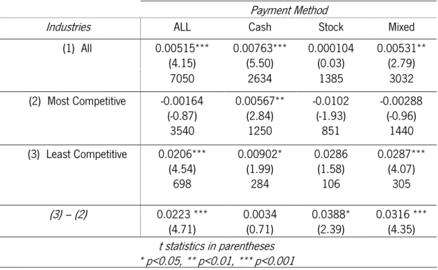
decrease at the lower levels of competitions due to a reduction of the information asymmetry. Table 5 shows the CARs by the payment method for all, the most and least competitive industries. Overall, the earnings are all positive, independently of the payment method. As expected, all-cash has the highest returns, 0.76%, followed by the mixed payment, 0.53%, and in the bottom, there’s the all-stock payment, 0.01%. Cash and mixed payments have significant values.
Moving to the top 3 most competitive industries, the distribution of the CARs remain the same. Cash payments are the only payment method with a statistically significant return with 0.567% of CARs. The remaining methods display negative values. Differently, in the least competitive industries, all, cash and mixed have statistically significant returns, yet, unlike the previous situation where cash was the most positive, here it is the least positive. The overall payments have positive returns averaging a 2.06% income, the mixed method has the highest earnings, 2.87%, and cash has 0.902%. All the mentioned are significant at 5%. Despite the non-significant returns, stock payments go from negative to null.
Regarding the differences between the least and most competitive, there are substantial values that highlight the change showed previously. The differences are 2.23%, 0.34%, 3.88% and 3.16% for the average, cash, stock and mixed payments respectively. All the differences are positive and significant, except for the cash payment. Firstly, the progress of the table shows and enlightens the positive aspect of the cash payments, because independently of the competition degree the CARs are always positive. Secondly, returns with the equity payment are the ones with the largest variation, suggesting that the degree of competition has a good bearing on the equity payment, dominating the negative effect of the information asymmetry. Finally, somewhat like equity payments, the mixed method seems to also affect positively by a reduction in competition.
Table 5- Acquirer’s CARs by the payment method. CARs are calculated using the event study. It is split between the all, most competitive and least competitive using the proxy of competition of Alexandridis et al. (2010). The most competitive industries are Business equipment, telecommunications and energy. The least competitive are Chemicals, Shops and Consumer Durables. cash payment is deals using 100% of the cash. Stock is deals using 100% of the stock. Mixed is the remaining deals. Values below the t statistics are the number of observations.
5.2.2- Target returns by payment method across the different levels of Competition
All the targets’ returns are expected to be vastly positive regardless of the degree of competition, and when equity is used the abnormal returns are expected to be lower than the outstanding methods. Table 6 shows precisely that. Firstly, the sample total average is 26.2% and cash payments are 34.3%. This underlines the favourable impact of cash once more. Further, I confirm the negative influence of the equity on acquisitions, since stock payment has the lowest returns of all with 17.4%.
Inside the sectors with the most M&As, returns are lower than the overall sample apart from the equity payment. Further, cash payments continue to have the highest returns with CARs of 33% and equity has the lowest CARs with 17.6%. Moving to panel 3, where only the least competitive sectors are examined. The CARs are comparable to the literature. As expected, the cash and the stock payments exhibit the highest and the lowest earnings, 32.2% and 11%, respectively.
Payment Method
Industries ALL Cash Stock Mixed
(1) All 0.00515*** 0.00763*** 0.000104 0.00531** (4.15) (5.50) (0.03) (2.79) 7050 2634 1385 3032 (2) Most Competitive -0.00164 0.00567** -0.0102 -0.00288 (-0.87) (2.84) (-1.93) (-0.96) 3540 1250 851 1440 (3) Least Competitive 0.0206*** (4.54) 0.00902* (1.99) 0.0286 (1.58) 0.0287*** (4.07) 698 284 106 305 (3) – (2) 0.0223 *** 0.0034 0.0388* 0.0316 *** (4.71) (0.71) (2.39) (4.35) t statistics in parentheses * p<0.05, ** p<0.01, *** p<0.001
Further, the mixed method is the only that has a positive difference and the only with a significant difference, contradictory to the literature (Alexandridis et al., 2010). This finding is inconclusive because only one payment method has a significant difference while the remaining have null differences. Perhaps, the differences between markets are responsible for the CARs’ variations and not due to the corporate competition at the industry level. Going alongside the previous hypothesis results.
Table 6- Target’s CARs by payment method. CARs are calculated using the event study. It is split between the all, most competitive and least competitive using the proxy of competition of Alexandridis et al. (2010). The most competitive industries are Business equipment, telecommunications and energy. The least competitive are Chemicals, Shops and Consumer Durables. Cash payment is deals using 100% of the cash. Stock is deals using 100% of the stock. Mixed is the remaining deals. Values below the t statistics are the number of observations.
Payment Method
Industries All Cash Stock Mixed
(1) All 0.262*** 0.343*** 0.174*** 0.234*** (43.66) (36.93) (15.88) (23.73) 1681 687 450 544 (2) Most Competitive 0.250*** 0.330*** 0.176*** 0.203*** (29.58) (26.19) (11.57) (14.27) 782 336 234 212 (3) Least Competitive 0.260*** (13.29) 0.322*** (10.97) 0.110*** (3.48) 0.270*** (8.21) 156 68 32 56 (3) – (2) 0.01 -0.008 -0.066 0.067* (0.49) (-0.27) (-1.55) (2.08) t statistics in parentheses * p<0.05, ** p<0.01, *** p<0.001
5.3- Firm size
5.3.1- Returns by Acquirer size
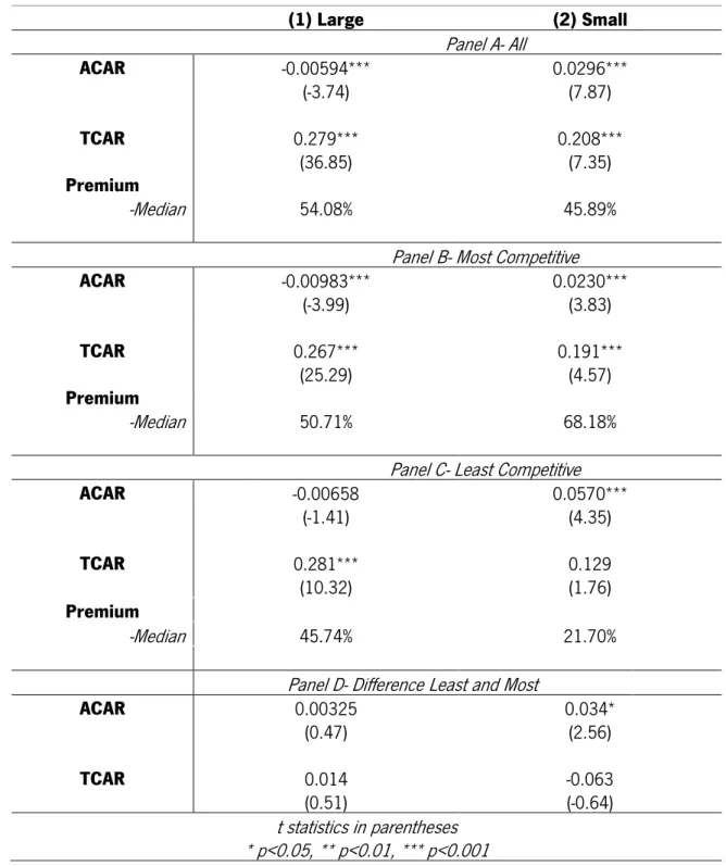
Table 7 displays the distribution of the returns by acquirer size. If large bidders systematically overpay, there’s a possibility that the market of corporate control fails to reduce the overpayment potential. Overall, large acquires pay a 54.08% (median) premium while small bidders pay 45.89%. The sample results are consistent with the literature. Large firms tend to overpay, consequently, generating lower returns to them and benefiting the targets due to the higher premium. Further, small and large acquirers have significant CARs at 2.96% and -0.59%,
respectively. Targets that were acquired by a large (small) firm had a 27.9% (20.8%) returns at the announcement. Essentially, the undersized bidders will always overperform the large bidders, this is a well-documented outcome known as the size effect. In this analysis the small-sized firms are only used as a premium comparison, measuring if overpayment happens or not.
Moving down in the panels, the situation inside the most competitive industries changes. Large firms have a decreasing on the overpayment, yet, continue to do it. Consequently, the CARs remain negative and significant, -0.98%, and even more negative than the panel A. Furthermore, despite the premium difference of almost -18%, their targets have higher earnings, 26.7%, than those acquired by small-scaled firms, 19.1%. In the least competitive, the initial overpayment by large bidders’ declines going from the initial 54.08% to the current 45.74%, but still overpays by comparison to the small-scale firms. As expected, targets have vast earnings if their counterpart has a higher dimension. Large firms display returns of -0.658% while small firms have 5.7% of returns.
Comparing the two subsamples of the industries, the small-scaled firms are the clear winners, going from the most to the least competitive their returns rise by 3.4%. Moreover, the acquirer’s CARs go from the previous negative and significant, 0.98%, to the null value of -0.658%. For the targets, the differences are negative and positive for the large and small acquirers, respectively. Firstly, this finding proves the overall negative effect of the bidder size for the acquirer’s CARs and the positive effect on the target’s returns. Secondly, the results suggest that acquirer’s CARs are worse for large firms in highly competitive industries. On the other side, it also suggests that targets enjoy better returns in most competitive industries when they are purchased by firms with high evaluations.
Table 7- CARs by acquirer size. It is split between the all, most competitive and least competitive using the proxy of competition of Alexandridis et al. (2010). The most competitive industries are Business equipment, telecommunications and energy. The least competitive are Chemicals, Shops and Consumer Durables. CARs are calculated using the event study. ACAR is the acquirer’s cumulative abnormal returns. TCAR is the target’s cumulative abnormal returns. Large stands for large bidders, thus, the acquirer’s that have a higher market value 4 weeks before the announcement than the 75th percentile of the yearly market value of all the listed firms within each industry. Small stands for small bidders, thus, the acquirer’s that have a lower market value 4 weeks before the announcement than the 25th percentile of the yearly market value of all the listed firms within each industry. Premium is the ratio of the transaction value over the target’s market value 4 weeks before the announcement.
(1) Large (2) Small Panel A- All ACAR -0.00594*** 0.0296*** (-3.74) (7.87) TCAR 0.279*** 0.208*** (36.85) (7.35) Premium -Median 54.08% 45.89%
Panel B- Most Competitive
ACAR -0.00983*** 0.0230*** (-3.99) (3.83) TCAR 0.267*** 0.191*** (25.29) (4.57) Premium -Median 50.71% 68.18%
Panel C- Least Competitive
ACAR -0.00658 0.0570*** (-1.41) (4.35) TCAR 0.281*** 0.129 (10.32) (1.76) Premium -Median 45.74% 21.70%
Panel D- Difference Least and Most
ACAR 0.00325 0.034* (0.47) (2.56) TCAR 0.014 -0.063 (0.51) (-0.64) t statistics in parentheses * p<0.05, ** p<0.01, *** p<0.001
5.3.2- Returns by Target Size
5.3.2.1- Bidder CARs by Target Size across the different levels of Competition
Table 8 displays the relation between the bidder’s CARs and the premium with the natural logarithm of the deal size variable, LNMKRT. Deal size as the ratio of the target size and the yearly market value median of all the listed firms inside each industry. Companies that acquire big targets are supposed to have negative returns, despite the lower premium. Looking at the results of the regressions, the acquisition premium is negatively related to the size, thus, bigger companies receive a lower premium than smaller ones. Furthermore, the CARs are also negatively associated with target size, for that reason I anticipate negative returns for firms that attain bulky targets.
Table 8- Displays the regressions using Premium and the acquirer’s CARs as in the dependent variable, both with the LNMKRT independent variable. LNMKRT is the natural logarithm of target market value 4 weeks before the announcement over the median of all the listed firms inside each industry. Premium is the ratio of the transaction value over the target’s market value 4 weeks before the announcement.
Table 9 displays the acquirer’s returns by target size. At this point, the sample only contains public acquisitions due to the target’s information availability. Independently of the target's size,
bidders have negative returns, something very common with public acquisitions. Curiously, for
the overall sample and subsamples, small targets seem always to generate returns around -1%. At the panel (1), all the coefficients are negative and significant. Confirming that when acquirers procced to do an M&A of a public firm the gains are not beneficial. Within the most competitive subsample, all the returns are negative, especially the acquires that purchased big targets and
(1) (2) Premium CAR Intercept 0.700*** -0.0173*** (23.61) (-7.45) LNMKRT -0.187*** -0.00426*** (-12.51) (-3.63) t statistics in parentheses * p<0.05, ** p<0.01, *** p<0.001
sample has abnormal, returns of -0.182% and the bidders that acquired large firms have negative CARs, of -2.35%.
Looking at the differences, only the overall sample has a positive and significant value with a variation of 2.05%. Accordingly, this confirms the disadvantaged that is the level of competition on the acquirers’ earnings. Further, despite the non-significant variation on both the size-related subsample, the difference of the acquirer’s CARs that purchased big targets went from significant to not significant as the level of competition decreased. Implying that the combination of the deal size and the competition does have some impact, yet, not large enough to produce a change in the nature of the CARs.
Table 9- Acquirer’s CARs by Target size. CARs are calculated using the event study. It is split between the all, most competitive and least competitive using the proxy of competition of Alexandridis et al. (2010). The most competitive industries are Business equipment, telecommunications and energy. The least competitive are Chemicals, Shops and Consumer Durables. Big stands for the large targets. Small stands for small targets. The size of the targets is calculated using the ratio of the market value of the target 4 weeks before the announcement over the yearly median of all market values by industry. Therefore, those with a value higher than the 75th percentile are considered big and those with lower values than the 25th percentile are considered small.
5.3.2.2- Target returns by Target Size across the different levels of Competition
Table 10 shows the targets’ CARs divided by the target size. All the returns are positive and significant for all industries, inside the most competitive and in the least competitive.
Target Size
Industries All Big Small
(1) All -0.0149*** -0.0342*** -0.0109* (-6.67) (-6.14) (-2.51) (2) Most Competitive -0.0224*** -0.0475*** -0.0117 (-6.75) (-4.83) (-1.79) (3) Least Competitive -0.00182 (-0.23) -0.0235 (-1.55) -0.0170 (-1.18) (3) – (2) 0.0205* 0.024 -0.0053 (2.52) (1.05) (-0.35) t statistics in parentheses * p<0.05, ** p<0.01, *** p<0.001
Furthermore, big targets have lower returns than the small ones, probably due to the lower received premium and other factors, such as the complexity level of the post-merger integration. This behaviour holds for all industries, inclusively when individually examining the most and least competitive. At the overall sample, the CARs average for big targets is 18.5%. Interestingly, in the most competitive sectors, where the returns should be higher due to the larger premium, all the abnormal returns decrease by at least 1%. Now, inside the least competitive subsample, the overall sample and the small targets increase compared to the previous tier. Only, the big targets have lower returns, going from 17.4% of the most competitive subsample to the current 15.6%. Most likely, this happens due to the lower premium paid. Also, looking to the table, I confirm the broad negative influence of the deal size on the returns throughout the different levels of competition. Finally, looking at the differences panel, the difference is negative for the big targets, although, is not significant. Going alongside the results from the other univariate tests.
Table 10- Target’s CARs by Target size. CARs are calculated using the event study. It is split between the all, most competitive and least competitive using the proxy of competition of Alexandridis et al. (2010). The most competitive industries are Business equipment, telecommunications and energy. The least competitive are Chemicals, Shops and Consumer Durables. Big stands for the large targets. Small stands for small targets. The size of the targets is calculated using the ratio of the market value of the target 4 weeks before the announcement over the yearly median of all market values by industry. Therefore, those with a value higher than the 75th percentile are considered big and those with lower values than the 25th percentile are considered small.
Target Size
Industries All Big Small
(1) All 0.262*** 0.185*** 0.315*** (43.66) (15.69) (23.87) (2) Most Competitive 0.250*** 0.174*** 0.297*** (29.58) (10.88) (14.91) (3) Least Competitive 0.260*** (13.29) 0.156*** (4.29) 0.306*** (7.82) (3) – (2) 0.01 -0.018 0.0093 (0.49) (-0.47) (0.21) t statistics in parentheses * p<0.05, ** p<0.01, *** p<0.001
5.4- Multivariate analysis
Broadly speaking, the results from the univariate tests proposes that clearly, the acquirers benefit the greatest in the least competitive industries, as documented in the literature. On the other side, targets’ returns go under very slight changes between the two degrees of competition. Regardless, only through the univariate analysis is not possible to confirm if the changes are due to the competition and not due to other factors.
In this section, I do a multivariate analysis using the acquirers’ and targets’ CARs as the dependent variables. Based on my previous results, I expect that the level of competition to be negatively associated with the acquirers’ returns. The main explanatory variable is the time-varying competition dummy that takes the value of 1 if a certain industry is in the top 3 most competitive of that year and 0 otherwise. It is measured using the ratio of listed targets and listed firms by industry, consequently, the use of the industry fixed effects is not required. Additional to the main explanatory variable, I use the interaction between the competition and different dummies allied to the preceding hypothesis, allowing me to see its direct bearing on the returns related to the stock payment, acquirer size and target size.
Table 11 exhibits the multivariate analysis of acquirers’ CARs. Each analysis phase is separated
into the sample, the public and the private acquisitions. The public has two regressions due to
the full collinearity of the bidder size and the target size. Firstly, in the regressions (1)-(4) the coefficients of the competition are negative and significant. For an increase of 1% on the level of competition the CARs will decrease by 2.47% for the whole sample. This proves the well-documented effect of competition on acquirers’ CARs (Alexandridis et al., 2010). Moreover, using equity as payment in public acquisitions has been documented to destroy value for the acquirers (Travlos, 1987; Fuller et al., 2002; Moeller et al., 2004). The main school of thought supports that it happens due to information asymmetry, where the target’s manager perceives the equity offering as overvalued (Travlos, 1987; Alexandridis et al., 2010). Still, this effect only holds for public purchases. Private buying prospers on the usage of equity because there’s less information about the target (Hansen, 1987). In the regressions (1)-(4) the stock's coefficient is
negative, apart from private acquisition, and it is statistically significant for the public M&As. It
confirms the literature on the matter. Additionally, looking at the interaction between the competition and the stock variable the value is negative for public and positive for the overall and private acquisitions.
As demonstrated by Moeller et al. (2004), large firms overpay while small don’t. Theoretically, this should hold for both types of acquisitions. Moreover, large bidders rather use stock than cash as payment (Dong et al., 2006; Moeller et al., 2004), so the negative effect of the acquirer size can be enhanced even more. I expect that within the most competitive industries the coefficients are worse than in the least competitive subsample because their acquirer size is significantly larger. Accordingly, looking at the bidder size variable, the number is negative and always significant through (1)-(4) regressions. Confirming that the overpayment destroys the earnings of the acquiring firms. Linking the level of competition to large acquirers. The sample and private regressions have statistically significant and positive values. Therefore, when an industry is in the top 3 of the most competitive sectors and a large acquirer proceeds to buy a private firm, its CARs rises 1.50% by each unit increase of competition level. On the regression (3) is added the deal size and the dummy competition x deal size and consequently, the removal of the variables related to the bidder size. Due to the nature of the acquisition and the information availability, the deal size is only tested on public M&As. The variable has a significant and negative coefficient, thus, targets with high valuations induce lower returns to their acquirers. The interaction between the competition dummy and the deal size has a negative value.
Additionally, when buying public firms the acquirer’s CARs decrease as the relative size increases (Jensen & Ruback, 1983; Travlos, 1987; Alexandridis et al., 2010), where relative size is the transaction value divided by the bidder’s market value 4 weeks before the announcement. Fuller et al. (2002) confirm this effect is only for the stock payment. Growths in the relative size generate better revenues if buying private targets and especially when equity is used (Fuller et al., 2002). Regressions (1)-(4) have positive and negative values, both significant, for the private and
public acquisitions, respectively. It proves its negative effect on public acquisition and the positive
relation with the private M&As. A possible explanation is that the effect is stock driven (Fuller et al., 2002). For the negative effect of the relative size on public acquisition is that large acquirers not only rather use the stock as payment but also systematically overpay, increasing the relative size. On the other hand, private acquisitions are connected positively to the stock payments, thus, increases on the relative size are positive to the earnings.
Regarding the nature of the transaction, private acquisitions cause positive returns (Chang, 1998; Fuller et al. et al., 2002; Mitchell et al., 2004; Moeller et al., 2004; Faccio et al., 2006;). Throughout most regressions, the private variable is always significant and positive confirming
Lastly, in the past years more and more acquisitions have been horizontal, inside the same industry. Therefore, I examined if the inter-industry acquisitions have a negative impact and, thus, explaining the surge in the horizontal acquisitions. From (1)-(4) the coefficients of the overall and the privates M&As are negative and significant values. Therefore, horizontal acquisitions in the private sector decrease CARs.
In the regressions (5)-(8), I apply all the previous variables to the subsample of the most competitive industries. Most of the control variables continue to exhibit the prior performance, with the exclusion of the interindustry variable that now is always negative. Moreover, the stock variable has negative coefficients while its interaction with the competition dummy displays the same distribution as the in regressions (1)-(4). The bidder size has a negative and significant effect on the returns, for all acquisitions again. More, when interacting with the bidder size and the competition large firms that purchase privately continue to display the same positive and important influence, as previously shown. Reaffirming the listing effect. Concerning the deal size, its effect continues to be harmful and significant, as it was before for the full sample. The dummy competition x deal size has a positive value. Lastly, the competition variable remains negative for the 4 regressions but only significant for the overall sample and the private purchases. Hence, I confirm that the competition effect still holds at this subsample.
The regressions (9)-(12) applies the prior analysis to the least competitive subsample. The competition coefficient is now positive for private purchases and negative for public M&As, both are significant. Therefore, the situation remains the same as before for the public sector, while the private sector is affected positively by the competition level at the current subsample. Accordingly, increases in the competition seem to rise the CARs of the purchasing firm when buying privately, if the least competitive industry become one of the most competitive. All the stock values are negative. Also, the dummy competition x stock that shows the impact of the stock on the increasing competition has positive and significant for the overall sample and the private purchases. Apart from the public sector, the bidder size has a negative and its interaction with the competition dummy is positive. The deal size is negative while the dummy competition x deal size is positive. Regarding the relative size, the value is always positive, and it is significant for the overall sample. Like before. The combination with the competition shows both the public and private M&As have their CARs impacted significantly. The effect of the relative size on the private purchases is still beneficial, yet, it is even more advantageous and significant with the
increasing of the competition. On the other side, public M&As have their earnings even more reduced. The remaining control variable continues to display the same impact as before.
Alexandridis et al. (2010) proved that the differences in CARs, of public M&As, was due to the competition and not due to differences between the markets and with this multivariate analysis I also confirm it. Notwithstanding, as a robustness check, instead of using the competition dummy that takes the value of 1 when an industry is in the top 3 of the most competitive of that year, I use a percentual time-varying competition variable. The measurement method is the same but in the place of 1 and 0, it has the percentage that shows the number of listed acquired targets over the total number of listed firms by each year. Accordingly, all the results continue to display the
Table 11- Displays the multivariate analysis using the acquirer’s CARs as the dependent variable and the competition as the main explanatory variable. It is split between the all, most competitive and least competitive using the proxy of competition of Alexandridis et al. (2010). The most competitive industries are Business equipment, telecommunications and energy. The
least competitive are Chemicals, Shops and Consumer Durables. Regressions (1)-(4) are using the sample, (5)-(8) is using only the most competitive industries and (9)-(12) using the least
competitive. Each phase is divided into All targets, public targets and private targets. Competition is a time-varying dummy that takes the value of 1 when the industry is on the top 25% of the most competitive. Stock is a dummy that takes the value of 1 one the deals is closed using only stock. Dummy competition x stock is the interaction between the competition dummy and the stock variable. Bidder size is the natural logarithm of the acquirer’s market value 4 weeks before the announcement. Dummy competition x bidder size is the competition dummy times the variable that takes the value of 1 if the acquirer is large. An acquirer is considered large if it’s market value 4 weeks before the announcement is higher than the 75th percentile of all the listed firms by industry and year. Deal size is the ratio target’s market value 4 weeks before the announcement over the median of the market values of each industry and by year. Dummy competition x deal size is the competition dummy times the variable that takes the value of 1 if the target is big. A Target is considered big if it’s deal size ratio is higher than the 75th percentile of all the listed firms by industry and year. Relative size is the natural logarithm transaction value over the acquirer’s market value 4 weeks before the announcement. Dummy competition x relative size is the interaction of the competition dummy with the relative size variable. Private is a dummy that is 1 when the acquisition is private. Multiples bidder is a dummy for acquisitions that had more than one bidder. Interindustry is a dummy that takes a value of 1 when the acquisition is between different industries. Industries were defined using the SIC codes of the 12 industries of Fama & French, apart from the Financial sector. n is the number of observations.
1 2 3 4 5 6 7 8 9 10 11 12
All Public Private All Public Private All Public Private
All Most Competitive Least Competitive
Competition -0.0247*** -0.0193* -0.0188* -0.0215*** -0.0243** -0.0111 -0.00897 -0.0219* 0.0215 -0.101** -0.126*** 0.0698**
(-5.23) (-2.32) (-2.31) (-3.71) (-2.90) (-0.75) (-0.61) (-2.16) (1.18) (-2.96) (-3.58) (3.27)
Stock -0.00916 -0.0297*** -0.0259*** 0.000793 -0.0164 -0.0203 -0.0127 -0.0151 -0.0226 -0.0289 -0.0271 -0.0217
Dummy Competition x Stock 0.00198 -0.00841 -0.00932 0.00549 0.00624 -0.0222 -0.0276 0.0178 0.0822** 0.0383 0.0549 0.0902** (0.31) (-0.81) (-0.90) (0.69) (0.61) (-1.24) (-1.57) (1.44) (2.71) (0.62) (0.92) (2.63) Bidder Size -0.00355** * -0.00449** -0.0026** -0.00402** -0.00517* -0.00340* -0.00197 0.00159 -0.00335 (-4.45) (-3.19) (-2.68) (-3.18) (-2.33) (-2.20) (-0.80) (0.33) (-1.16) Dummy Competition x Bidder Size 0.0109* -0.000434 0.0150** 0.00974 -0.0108 0.0177* 0.0171 -0.0130 0.0483 (2.41) (-0.05) (2.61) (1.57) (-0.98) (2.31) (0.65) (-0.24) (1.50) Deal Size -0.00138** * -0.00432** * -0.000215 (-3.52) (-4.15) (-0.27) Dummy Competition x Deal Size -0.000750 0 0.0161 0.0415 (-0.07) (1.03) (0.63) Relative size 0.0066*** -0.00433* -0.000951 0.0103*** 0.00647** -0.00887* -0.00443 0.0101*** 0.00690* 0.00593 0.00568 0.00683 (5.42) (-1.98) (-0.48) (6.99) (2.73) (-1.97) (-1.06) (3.57) (2.15) (1.06) (1.20) (1.79)
Dummy Competition x Relative Size -0.0045** -0.00303 -0.00308 -0.00309 -0.00654* -0.00145 0.000077 -0.00513 0.00865 -0.0254 --0.0278* 0.0226** (-2.94) (-1.10) (-1.16) (-1.63) (-2.55) (-0.30) (0.02) (-1.67) (1.35) (-1.91) (-2.60) (3.05) Private 0.021*** 0.0215*** 0.0225 (6.12) (4.12) (1.95) Multiple Bidders -0.00677 -0.00424 0.00156 -0.0111 0.0165 0.0162 0.0219 -0.00918 -0.000345 -0.00181 -0.00134 (-0.59) (-0.40) (0.15) (-0.21) (0.90) (0.97) (1.33) (-0.14) (-0.01) (-0.06) (-0.04) Inter-industry -0.00555* 0.000549 0.00183 -0.0085** -0.00308 -0.0105 -0.00648 -0.00319 -0.000768 0.00706 0.00484 -0.00789 (-1.98) (0.10) (0.33) (-2.64) (-0.55) (-0.99) (-0.61) (-0.49) (-0.09) (0.41) (0.27) (-0.77) Intercept 0.0364*** 0.0298** 0.00195 0.0603*** 0.0310** 0.0241 -0.00606 0.0563*** 0.0279 0.0103 0.0226 0.0569*** (5.71) (2.63) (0.33) (10.76) (2.82) (1.18) (-0.47) (5.38) (1.46) (0.30) (1.64) (3.68) N 7050 1702 1638 5348 3540 818 784 2722 695 167 160 528