WO R K I N G PA P E R S E R I E S

WO R K I N G PA P E R S E R I E S

N O 7 7 5 / J U LY 2 0 0 7

OF BUDGET COMPONENTS

AND OUTPUT

by António Afonso

In 2007 all ECB publications feature a motif taken from the

€_{20 banknote.}

WO R K I N G PA P E R S E R I E S

N O 7 7 5 / J U LY 2 0 0 7

1 We are grateful to Luís Costa, Arne Gieseck, Michael Thöne, Jürgen von Hagen, Jan in‘t Veld and two anonymous referees for helpful comments. We also thank seminar participants at the ECB, at ISEG/UTL, at the 61st _{European Meeting of the} Econometric Society, and at DG ECFIN for further discussions. Valuable assistance of Renate Dreiskena with the data is highly

THE DYNAMIC BEHAVIOUR

OF BUDGET COMPONENTS

AND OUTPUT

1

by António Afonso

2

and Peter Claeys

3

© European Central Bank, 2007

Address

Kaiserstrasse 29

60311 Frankfurt am Main, Germany

Postal address

Postfach 16 03 19

60066 Frankfurt am Main, Germany

Telephone

+49 69 1344 0

Internet

http://www.ecb.int

Fax

+49 69 1344 6000

Telex

411 144 ecb d

All rights reserved.

Any reproduction, publication and reprint in the form of a different publication, whether printed or produced electronically, in whole or in part, is permitted only with the explicit written authorisation of the ECB or the author(s).

The views expressed in this paper do not necessarily reflect those of the European Central Bank.

CONTENTS

Abstract 4

Non-technical summary 5

1 Introduction 7

2 The recent fiscal imbalances in the EU 8

3 An SVAR model for gauging fiscal indicators 10

3.1 Fiscal indicators 10

3.2 Towards an economic indicator of

fiscal policy 11

3.3 Methodology 13

3.4 Gauging the fiscal indicator 16

4 Empirical analysis 19

4.1 Data 19

4.2 The transmission channels of fiscal policy 20

4.3 The fiscal indicator 24

4.4 Some sensitivity analysis 27

5 Conclusion 31

References 33

Figures 36

Appendix 1. Data sources 43

Appendix 2. The fiscal indicator:

some additional results 44

Abstract

The main focus of this paper is the relation between the cyclical components of total revenues and expenditures and the budget balance in France, Germany, Portugal, and Spain. We try to uncover past trends behind the development of public finances that contribute to explaining the current stance of fiscal policy. The disaggregate analysis of fiscal policy in an SVAR that mixes long and short-term constraints allows us to look into the transmission channels of fiscal policy and to derive a model-based indicator of structural balance. The main conclusions are that fiscal slippages are mainly due to reversals in tax policies, which are unmatched by expenditure adjustments. As a consequence, deficits rise when economic conditions worsen but cause a ‘ratcheting up’ in the size of government in economic booms. The Stability and Growth Pact has not eradicated these procyclical policies. Bad policies in good times also contribute to aggregate macroeconomic instability.

Non-technical summary

In recent years, we have witnessed a worldwide swing towards fiscal profligacy. In the US,

budget deficits have suddenly widened since 2001 after the tax cuts of the Bush

Administration. In the European Union, mounting budget deficits have come somewhat as a

surprise as the Maastricht Treaty and afterwards the Stability and Growth Pact seemed to

have put in place a set of tight fiscal rules. A combination of a 3% deficit rule, a commitment

to keep structural deficits close to balance or even in surplus, together with a peer revision of

fiscal stance through the Excessive Deficit Procedure were considered as a guarantee for

the sustainability of public finances. After the initial application of the Excessive deficit

Procedure to Portugal, France and Germany, there was a breach of the 3% deficit limit in

several other EU countries. A revised version of the Stability and Growth Pact was

negotiated in March 2005.

A variety of political and economic factors probably underlie the observed rise in public

deficit and debt ratios. We try to uncover underlying past trends behind the development of

public finances that may contribute to explaining the recent budgetary outlook in France,

Germany and Portugal. These countries were subject to several steps of the Excessive

Deficit Procedure as deficits rose above the 3% limit. We are particularly interested in the

underlying causes of the breach of the Pact’s rules by looking into adjustments in both

spending and revenues. At the same time, we look into how these adjustments contribute to

the long-term growth prospects and outlook for the sustainability of public finances. For this

reason, we also consider Spain, as it kept the budget close to balance. We are interested in

the economic reasons of such a vigorous fiscal management.

To that end, we construct a model-based indicator of structural balance by combining

insights from two different strands of the empirical VAR literature. There is a growing

empirical literature on the effects of fiscal policy, which is modelled with structural VARs

(Blanchard and Perotti, 2002). The basic approach in this literature is to capture

discretionary fiscal adjustments by filtering out the fiscal balance for cyclical reactions of

different budget items. A recent theoretical literature argues on the importance of long-term

growth effects of both taxation and specific spending items. The main message of

endogenous growth models with fiscal policy is that higher taxation unambiguously reduces

output, but that such losses may be offset, by using the proceeds for productive spending

items (Barro, 1990; King and Rebelo, 1990, Turnovsky, 2000). Our approach innovates on

existing evidence of the fiscal SVAR models in using a mixture of short and long-term

economic growth and fiscal variables. This allows for permanent shocks to determine

trending behaviour of output and fiscal variables à la Blanchard and Quah (1989). Like

Blanchard and Perotti (2002), we filter the fiscal balance for cyclical reactions of spending

and revenues to obtain the discretionary fiscal shock. In this paper, we examine aggregate

spending and revenues. More elaborate models might incorporate refinements of the

composition of budget balance.

Our indicator of structural fiscal balance is determined by the effect of permanent output and

discretionary fiscal shocks. Cyclical fluctuations are due to temporary economic shocks. This

stands in contrast to statistical methods for cyclically adjusting fiscal balances where the

cyclical elasticity of the budget is multiplied with an independently derived measure of the

output gap. The quantitative indicator that we obtain is best seen in the light of the growing

theoretical literature on the effects of fiscal policy. Dynamic stochastic general equilibrium

models with nominal rigidities offer a rationale for fiscal stabilisation policies. But these New

Keynesian models attribute a major role to the supply side effects of fiscal policy

adjustments. Our indicator is consistent with such a distinction. In contrast to statistical

models for adjusting fiscal balance, our economic indicator of structural balance has also

some attractive practical properties. Uncertainty on the stance of fiscal policy is explicitly

quantified. The theoretical assumptions underlying the model can be explicitly tested. Also,

the end-of-sample problem is reduced. The application of the model is not necessarily more

demanding in terms of data availability.

The main result of our study is that both the fiscal consolidations undertaken after Maastricht

and the mounting deficits since the start of the EMU are due to insufficient adjustments in

revenues. Governments generally cut tax rates during economic boom, but do not curtail

spending equally. The overall budget position seems in balance, but structural deficits build

up. As a consequence, deficits surface again when economic boom turns into bust.

Governments then reverse previous tax cuts to avoid mounting deficits. Over the period

1999-2001, we observe this behaviour in all countries that sinned to the rules of the Pact.

Governments implement bad policies in good times. These policies have some negative side

effects. First, it leads to a ‘ratcheting up’ of spending over the economic cycle. Second,

these procyclical switches in fiscal policy induce macroeconomic fluctuations. We indeed

1. Introduction

In recent years, we have witnessed a worldwide swing towards fiscal profligacy. In the

European Union, this has come somewhat as a surprise as the Maastricht Treaty and

afterwards the Stability and Growth Pact seemed to have put in place a set of fiscal rules

that guarantee the sustainability of public finances. After the initial nuisance in applying the

Pact to Portugal, France or Germany, there was a breach of the 3% deficit limit in several

other EU countries. A revised version of the Pact was negotiated in March 2005. The new

budget rules offer a more flexible approach for curbing excessive deficits over a longer

period of time, and put the emphasis on the sustainability of public finances. As part of the

Lisbon Strategy, considerably more attention is given to the composition of budget

adjustments with a view to promoting economic growth.

A variety of political and economic factors probably underlie the observed rise in public

deficit and debt ratios. We try to uncover underlying past trends behind the development of

public finances that may contribute to explaining the recent budgetary outlook in France,

Germany, Portugal, and Spain. While the first three countries were subject to several steps

of the Excessive Deficit Procedure, Spain on the other hand can be seen as an example of

more vigorous fiscal management. We are particularly interested in the underlying causes of

the breach of the Pact’s rules by looking into adjustments in various budget components. At

the same time, we look into how these adjustments contribute to the long-term growth

prospects and outlook for the sustainability of public finances.

To that end, we construct a model-based indicator of structural balance by combining

insights from the growing empirical literature on the effects of fiscal policy – modelled with

structural VARs – with statistical methods for cyclically adjusting fiscal balances. Our

approach innovates on extant evidence in using a mixture of short and long-term restrictions

to identify economic and fiscal shocks in a small-scale empirical model in economic growth

and fiscal variables. This allows for permanent shocks to determine trending behaviour of

output and fiscal variables à la Blanchard and Quah (1989). Discretionary fiscal adjustments

are captured by filtering out the fiscal balance for cyclical reactions of budget items, following

Blanchard and Perotti (2002). As a first step, we examine total spending and revenues. More

elaborate models might incorporate refinements of the composition of budget balance.

The quantitative indicator that we obtain is best seen in the light of the growing theoretical

literature on the effects of fiscal policy. Dynamic stochastic general equilibrium models with

nominal rigidities offer a rationale for fiscal stabilisation policies. But these New Keynesian

indicator is consistent with such a distinction. In contrast to statistical models for adjusting

fiscal balance, our economic indicator of structural balance has some attractive practical

properties. Uncertainty is explicitly quantified; theoretical assumptions can be explicitly

tested. Also, the end-of-sample problem is reduced. The model is not necessarily more

demanding in terms of data availability.

The main result of our study is that both the fiscal consolidations undertaken after Maastricht

and the mounting deficits since the start of the EMU are due to adjustments in revenues.

Governments cut tax rates during economic boom, but do not curtail spending equally. As a

consequence, deficits surface again when economic boom turns into bust. Governments

then reverse previous tax cuts to avoid large deficits. This leads to a ‘ratcheting up’ of

spending over the economic cycle. This procyclical bias in fiscal policies has not been

eliminated with the Stability and Growth Pact. Governments still implement bad policies in

good times and this unnecessarily induces macroeconomic fluctuations. We indeed find that

fiscal policy has minor supply but rather large demand effects.

The remainder of the paper is organised as follows. In section two, we briefly review recent

fiscal developments in the EU, notably for the cases of France, Germany, Portugal, and

Spain. Our structural VAR approach towards disentangling these developments, and the

derivation of the fiscal indicator, is discussed in section three. Section four reports our

empirical results, and section five concludes the paper.

2. The recent fiscal imbalances in the EU

The fiscal framework of EMU has been considered a means for implementing fiscal

consolidation. However, recent developments in several Euro Area countries raise the

question as to whether fiscal sustainability is endangered, in view of rising deficits and debts

at a moment when the effects of ageing populations will have a further burdening effect. In

2005, Excessive Deficit Procedures (EDP) have been carried out for both France and

Germany, while yet another EDP was launched for Portugal. There are also ongoing

procedures for Greece and Italy, while several other EU Member States face a situation of

excessive deficit. Recent developments cannot be seen without taking into account past

actions and trends in public finances. We focus attention on the evolution of public finances

since 1970 in the countries that initially ’sinned’ to the Pact (France, Germany and Portugal).

For comparison, we consider Spain as an example of a more prudent fiscal management.

We report in Figure 1 the general government balance, and its breakdown in revenue and

following an increasing trend since the early seventies, notably in France, Portugal and

Spain. But the increases in spending have outdone the growth in revenues by far. Hence,

there has been a continuous deficit bias. There were some good reasons in 1991 to embark

on consolidation by establishing a 3% deficit target. The Maastricht rules have been effective

in constraining further buoyant expenditure rises. Less than commensurate rises in revenue

intake have led to persistent albeit gradually declining deficits. Since the start of EMU, fiscal

positions have started to slip away again. As to the reasons for the breach of the Stability

and Growth Pact, further expenditure rises in France and Portugal seem to blame, whereas

in Germany large revenue reductions unmatched by expenditure cuts have pushed the

deficit beyond the 3% threshold. Spain, on the other hand, stands out for its balanced

budget over recent years, which is the result of a sustained reduction in expenditures since

1993 that has levelled off in recent years.

[INSERT FIGURE 1 HERE]

These budget developments cannot be separated from economic conditions. The budget

balance can slip out of control owing to automatic stabilisers. In economic bust, revenues

are smaller than budgeted as tax bases contract. Similarly, expenses on unemployment

benefits and transfers are higher than expected. Figure 2 compares some measures of the

output gap and cyclically adjusted balances computed by the European Commission and the

OECD, as well as a trend series retrieved from directly applying a Hodrick-Prescott filter on

the deficit series.1

[INSERT FIGURE 2 HERE]

The start-up of the EDPs to these countries seems justified on account of worsening

structural balances. In all countries, economic conditions improved considerably at the onset

of EMU. The overall deficit was notably reduced as a result. But the reversal of positive

output gaps laid out the structural weakness of the balance in France, Germany and

Portugal. Expenditures exceed average revenues over the cycle. In contrast, Spain presents

a quite different picture. The budget has been brought close to balance, and is even in slight

surplus. A constant spending to GDP ratio has been matched by a gradual rise in tax

revenues.

1 _{The smoothing parameter has been set at 6.25, adjusting with the fourth power of the observation frequency}

3. An SVAR model for gauging fiscal indicators

There are a variety of reasons for which the cyclically adjusted balance does not properly

reflect the stance of fiscal policy. Its use in assessing fiscal balances is therefore debatable.

3.1. Fiscal indicators

The notion of structural balance is based on the premise that total output fluctuates around

some unobserved trend that depends on the long-term potential growth path of the

economy. In combination with some assumptions on the cyclical behaviour of fiscal policy,

this allows deriving a cyclically adjusted balance. Common practice at the European

Commission, IMF or OECD regards the determination of cyclical variation in output and the

cyclicality of the budget as two distinct problems.

First, the output gap usually comes from some trend-extraction procedure with a statistical

filter applied directly to real output. This decomposition in trending and cyclical components

is usually done with a band-pass filter. Alternatively, the output gap is calculated as the

distance from actual to potential output where the latter is based on a production function for

the aggregate economy.2 Second, a bottom-up approach is adopted for the derivation of the

cyclical elasticities of several budget items. The output elasticity of government revenues is

based on the properties of each tax item (viz. social security contributions, corporate,

personal and indirect taxes) and the elasticity of the tax bases to output. The cyclical

variability in spending is of relatively minor importance: only unemployment benefits are

adjusted for the cycle. Other budget components are assumed to be cyclically insensitive.

Table 1 gathers the elasticities from OECD for the major budget categories in the countries

we study. As in most other European countries, the cyclical elasticity of total net lending

varies around 0.50. Most of the variation in the budget comes from procyclical corporate and

personal taxes.

Table 1. OECD output elasticities of various budget items

France Germany Portugal Spain

total spending -0.11 -0.18 -0.05 -0.15

corporate tax 1.59 1.53 1.17 1.15

personal tax 1.18 1.61 1.53 1.92

indirect tax 1.00 1.00 1.00 1.00

social security contributions 0.79 0.57 0.92 0.68

net lending 0.53 0.51 0.46 0.44

Source: Girouard and André (2005).

2

Quite some uncertainty surrounds the computation of structural balances in this two-step

procedure. Depending on the skewness of the distribution of the moving-average weights in

the filter that is being applied and the phase of the economic cycle, trend output is biased

towards actual values especially towards the end of the sample. Another problem is posed

by structural breaks. Windfall revenues or unexpected spending are entirely included in the

structural balance if they have nothing else than ‘accounting’ effects. Filters distribute the

effects of a break forward and backward on the trend. But this problem is not limited to

statistical methods. Even if we use the production function or consider a deterministic trend

a reasonable approximation to potential output, incorporating shifts remains a problematic

issue. The production function approach moreover suffers from plenty of assumptions on

parameters and functional forms that make cumulative uncertainty rather large. The various

assumptions on budget elasticities are not as crucial for the cyclically adjusted balance, but

are nevertheless not less problematic. Implicitly, it is assumed that average budget

elasticities have a time-invariant linear relation to changes in the economy. We come back to

this in a sensitivity analysis in section 4.4.

3.2. Towards an economic indicator of fiscal policy

The main difficulty in interpreting the structural balance is the absence from economic

arguments to underpin the trend/cycle decomposition. There is an implicit assumption in the

filtering methods on the frequency of the business cycle and hence on trend output under

average economic conditions. And while the production function approach builds upon

economic foundations, the dynamics are nonetheless driven solely by the longer-term

effects of investment feeding back on changes in the capital stock.3

Macroeconomic models that allow for cyclical fluctuations around some steady-state

trending growth path can be found in the growing class of Dynamic Stochastic General

Equilibrium (DSGE) models with nominal rigidities. These models have by now been

extended to include fiscal policy. In the initial Real Business Cycle models, there are only

supply-side effects of fiscal policy that transmit through wealth effects and the labour/leisure

trade off (Baxter and King, 1993). Micro-founded models based on sticky prices provide a

rationale for fiscal stabilisation policies. But even in the New Keynesian type of models of

fiscal policy, the supply side effects still tend to dominate demand side effects of fiscal policy

management (Linnemann and Schabert, 2003). A larger role for demand side effects of

fiscal policy is only found in models that introduce some further imperfections via ‘Rule of

3

Thumb’ consumers or a fraction of liquidity constrained consumers (Galí et al., 2005; Bilbiie

et al., 2006).

The main result of studies that use the VAR-counterparts to DSGE-models is the significant

positive effect of fiscal expansions on output. The evidence is more in line with a positive

‘Keynesian’ effect on consumption, albeit the eventual multiplier is strongly reduced. The

identification of fiscal policy is fraught with difficulties, however (Perotti, 2005). First, the

implementation of announced changes in government policies is subject to lengthy and

visible political negotiations that are largely anticipated by private agents. As a

consequence, fiscal shocks need not affect fiscal variables first. This is a problem of the

shock being non-fundamental (Lippi and Reichlin, 1994). Second, these identification

problems are only exacerbated by the automatic reaction of fiscal aggregates to economic

variables. Finally, decisions on fiscal policy affect different groups in the public via a range of

different spending and tax instruments. There exists no ‘standard’ fiscal shock: every

political discussion considers the trade-off between a range of possible taxation and

spending adjustments. The means of financing and the adjustment in expenditures and

revenues wrap empirically relevant effects of different budget components in an aggregate

fiscal shock. Most studies focus on total spending or revenues, and find small and positive

effects of government spending on consumption, but prolonged negative effects of higher

taxation. Only a couple of studies consider the dynamic behaviour of some particular budget

components.

The seminal contribution of Blanchard and Perotti (2002) lies in using a semi-structural VAR

that employs external institutional information on the elasticity of fiscal variables to output.

By sorting out the automatic cyclical reaction of the total fiscal balance, discretionary shocks

to fiscal policy are nothing else than shifts to the cyclically adjusted balance. Blanchard and

Perotti (2002) additionally impose some timing restrictions on the economic effects of

discretionary policy. These timing assumptions avoid to some extent anticipation effects but

would not capture these completely if implementation lags are important.

The empirical literature has hitherto ignored the supply and demand channels of fiscal policy

that are at front-stage of the theoretical DSGE models. Such effects are only implicitly

acknowledged in these VAR studies. Changes in tax revenues, for example, are usually

found to have lasting effects on output. Some other strands of the empirical fiscal policy

literature have attributed a role to supply side developments. First, the literature on the

effects of fiscal consolidation would argue that large adjustments in fiscal policy that

contribute to restoring sustainability of public debt, might reverse the usual effects of fiscal

‘non-Keynesian’ output response (Alesina and Perotti, 1997). The effects of consolidation on

agents’ expectations on the future economic outlook – measured by asset markets’ reaction

(Giavazzi and Pagano, 1990) – suggests a role for permanent wealth and supply-side

effects of fiscal policy. Second, most VAR studies have ignored the literature on the

long-term growth effects of fiscal policies. The main message of endogenous growth models with

fiscal policy is that higher taxation unambiguously reduces output, but that such losses may

be offset, by using the proceeds for productive spending items (Barro, 1990; King and

Rebelo, 1990, Turnovsky, 2000). It can be argued that additional government spending in

catching-up countries such as Portugal and Spain had rather different effects than further

expansions of the budget in France and Germany, for example. This provides an additional

argument for including the former countries in our analysis.

The examination of the growth effects is also of substantial policy interest. In the

assessment of EU Member States’ policies under the revised Stability and Growth Pact,

much attention is devoted to the quality of fiscal adjustments and the sustainability of public

finances. The implementation of structural reforms that raise potential growth – and hence

have an impact on the long-term sustainability of public finances – can be considered

grounds for temporary deviations of budget balance. At the same time, the Pact’s account

for business cycle fluctuations, and allow for variations in the budget over the cycle. Our

framework distinguishes the longer run supply effects from this short-term variation in the

budget

3.3. Methodology

We make a first step in setting up an empirical VAR model that allows for fiscal policy having

distinct long- and short-term effects on output. The approach in this paper rests on a

combination of long-term restrictions and some assumptions on the short-run elasticities of

budgetary items.4 For the purpose of gauging a model-based fiscal indicator, we basically

take shocks with permanent effects on output to drive long-term trends. Following Blanchard

and Quah (1989), potential output is determined by so-called productivity or technology

shocks that permanently affect output. This can then be complemented with further

assumptions on the short-term behaviour of fiscal policies. Shocks with transitory output

effects are classified as either cyclical or fiscal, following the elasticity approach of Blanchard

and Perotti (2002).

4 _{A few other papers use similar restrictions for fiscal VARs, and are mostly inspired by a practical interest in}

We specify an empirical model of fiscal policy as a small-scale VAR in real output

y

_t and the

expenditure

g

t and revenue side

t

t of the government budget. We can summarise the data

properties in a VAR-model (1), ignoring for ease of notation any deterministic terms:

t t

X

L

B

(

)

=

ε

(1)

where

X

_t refers to the vector of variables

[

y

_t

g

_t

t

_t

]

, and

ε

_t contains the reduced form

OLS-residuals. By rewriting the VAR into its Wold moving average form (2),

t

t

B

L

X

=

(

)

−1

ε



t

′



t

 

. (2)

and imposing some structure on the relation between reduced form residuals

ε

t and

structural shocks

η

_t via the transformation matrix

A

(such that

A

ε

_t

=

η

_t), we can write the

model (2) as follows:

t t

t

C

L

B

L

A

X

=

(

)

η

=

(

)

−1

ε



t

′



t



I

. (3)

Any SVAR analysis needs to impose at least as much restrictions as contained in the matrix

A

to identify the model. By imposing orthogonality of the structural shocks we have already six (i.e. the covariance matrix of OLS residuals

Ω

=

AA

'

). Hence, we need to choose at least three more restrictions. The ones we employ are a combination of long and short-term

restrictions. The latter shape the contemporaneous relations among the variables through a

direct parameter choice on

A

. The former impose a long-term neutrality constraint on the effects of a structural shock

j

on some variable

i

. Those is, the i,j-th element of the infinite

horizon sum of coefficients, call it

C

(

1

)

_ij, is assumed to be zero. This requires an indirect

restriction in (3) on the product of the transformation matrix

A

and the inverted long-run coefficient matrix

B

(

1

)

−1. In other words,

[

C(1)

]

_ij =

[

B(1)−1A

]

_ij =0. (4)

For the system consisting of government expenditures, revenues and output, we assume

(

η

q) drives the long-term trend rise in output and leads to the unit root behaviour of real

output. This shock is isolated, by assuming there are two further shocks in the model that

both have temporary effects on output. I.e., we assume that

[

C

(

1

)

]

₁₂

=

0

and

[ ]

C

(

1

)

₁₃

=

0

in

(4). These shocks can be interpreted respectively as a generic business cycle shock (

η

c)

capturing short-term fluctuations around the moving steady state equilibrium for output, and

a fiscal shock (

η

f) with short-term ‘demand’ effects on output. In order to distinguish the

business cycle shock from the one to fiscal policy, we take up the elasticity approach

advocated by Blanchard and Perotti (2002). We derive a shock to spending and/or revenues

from which the cyclical variation has been removed. In other words, the shock with transitory

effects on output – but unaffected by short-term variation in output – is the fiscal policy shock

and reflects discretionary changes in the fiscal policy stance. We take elasticities for

government expenditures (

γ

) and revenues (

α

) with respect to output, and impose these

values on the relation in

A

between the reduced form residuals for output (

ε

y) and spending

(

ε

g) respectively revenues (

ε

t). The fiscal shock includes discretionary decisions that are unrelated to the cycle. Moreover, any government policy that interferes with the workings of

automatic stabilisers on a systematic basis is considered as a fiscal intervention.

Unlike other VAR studies, we split an overall change in fiscal policy into a part that has

short-term economic effects (the fiscal ‘demand’ shock), and into shocks that may have

potentially long-term growth effects (the ‘supply’ shock).5 An important limitation of the

current version of the model is that we cannot tell apart the growth effects coming from ‘pure’

technology shocks from those deriving from tax and spending decisions. Our supply shock is

a combination of all shocks with long-term output effects. The negative effects of

distortionary taxation or incentive-distorting spending contribute to this shock, as well as the

possibly positive effects of government investment. Instead, we isolate in the fiscal ‘demand’

shock only those changes in the discretionary budget stance that have temporary effects on

output. A full-fledged analysis of the economic growth effects of fiscal policy would require

additional restrictions.6 The current identification is sufficient though for the purpose of

deriving a fiscal indicator. We summarise our assumptions in Table 2:

We can not simply set to zero the elasticity

γ

of government expenditures. Unemployment

benefits move over the cycle in EU countries, even if their contribution to variation in total

5 _{For this reason, we do not expect responses to our fiscal shock to be similar to those documented in the}

empirical literature. Our distinction is more consistent with theoretical models of fiscal policy.

6

spending is not large. The parameter

γ

comes directly from the elasticities calculated by the

OECD that we reported in Table 1. In order to obtain the total elasticity of revenues

α

, we

subtract the spending elasticity (row 2 in Table 1) – accounting for its share in GDP – from

the elasticity of total net lending (row 7 in Table 1) instead of multiplying each revenue

category by its cyclical elasticity and GDP share. The coefficients do not sum to zero as the

budget is assumed to be countercyclical. Table 3 summarises our parameter assumptions.

Table 2. Identification in the long- and short-term

long-run restrictions

effect of shock on

Supply shock

q

η

Business cycle shock

η

c

Fiscal shock

f

η

real GDP

•

0 0

public spending

•

•

•

public revenues

•

•

•

short-run restrictions

Supply shock

q

η

Business cycle

shock

η

c

Fiscal shock

f

η

y

ε

•

•

•

g

ε

•

•

γ

t

ε

•

•

α

Table 3. Parameters γ and

α

France Germany Portugal Spain

total spending

γ

-0.11 -0.18 -0.05 -0.15

total revenues

α

0.58 0.59 0.47 0.49

3.4. Gauging the fiscal indicator

The structural model then permits adopting a unified approach towards contemporaneously

uncovering indicators of potential output

y

* and the structural balance

d

*. Basically, total output and government expenditures and revenues can be decomposed into the contribution

of each of the structural shocks. We take the stance that only supply shocks determine

potential output y_t* in the long term. Both fiscal shocks and supply shocks determine

structural expenditure gt* and revenues

*

t

t .7 Under this assumption, one can compute the

structural deficit as in (5):

* * * *

t t t t

y t g

d = − . (5)

7 _{Ultimately, the sustainability of fiscal policy is determined by the overall fiscal balance as well as potential}

This fiscal indicator

d

* can be interpreted as reflecting the discretionary stance of the fiscal authority. From the decomposition of the budget, we can then analyse whether such

changes usually occur via spending or taxation measures.

This measure cannot directly be compared to the cyclically adjusted balances provided by

the European Commission, OECD or those obtained with statistical filtering methods. Its size

and variability depends on the properties of shocks, which in our SVAR model carry an

economic interpretation. First, the output gap we derive need not correspond to the

fluctuations around a smooth trend on some assumption on the frequency of the business

cycle. The economic shocks that drive potential output reflect changes in technology. As

these supply shocks derive from a variety of sources, they likely vary over time. Our

approach is therefore best seen in the line of papers that investigate the role of nominal

versus technology shocks and give an economic interpretation to business cycle fluctuations

(Nelson and Plosser, 1982; King et al., 1991; Galí, 1992). Second, the variation in the

structural balance is different from that in traditional two-step methods. This discrepancy

owes to the definition of structural balance. This is best illustrated with an example. Consider

a cut in tax rates, for a given level of government spending and exogenous output. This

would lead to a deficit, ceteris paribus. If fiscal policy indeed has real economic effects as

the empirical literature suggests, then the tax cut temporarily boosts output. As a

consequence, spending on unemployment benefits decrease while the effect of lower tax

rates is to some extent offset by a larger tax base. Hence, revenues will increase and the

budget surplus will rise.

The traditional measure for cyclical adjustment takes out all cyclical variation, also the one

induced by fiscal policy, which leads to an overstatement of the structural balance. In our

approach, we control for this economic effect of the tax cut. The SVAR-model excludes that

part of the variation in GDP due to discretionary fiscal measures whereas standard models

take total output variation into account. But our approach goes even one step further.

Imagine that the tax cut also raises potential output in the long term (i.e., the tax cut is a

positive supply shock). This widens the gap between actual and potential output at the

moment the fiscal shock occurs. Structural balance would be improved as the increased tax

base (now, and in the future) makes the fiscal position more sustainable. Similar arguments

can be made for the effects of spending. Hence, our indicator is more relevant for the

assessment of the stance of fiscal authorities, with a view to the growth effects and

Our model-based indicator moreover has some favourable econometric properties in

comparison to more conventional measures. First, the simultaneous determination of a

measure of cyclical output and fiscal balance is more coherent. We only need to impose a

minimal set of economic restrictions to identify the model. These constraints are consistent

with recent DSGE models of fiscal policy that have at their core the supply and demand

effects of spending and tax decisions (Linnemann and Schabert, 2003; Galí et al., 2005).

The validity of these assumptions can be tested. While the method is definitely more

complex, total uncertainty is quantified. Sensitivity analysis can make clear the weakness of

the model in some specific direction. Moreover, progress in theoretical models of fiscal

policy can lead to further refinements of the approach. Second, by adopting an economic –

and not a statistical – method, the end-point problem of filters is eliminated. The indicator

gives timely information on changes in the fiscal stance.8

This has to be traded off against some weaknesses of the SVAR approach. First, extensions

are difficult as the method is rather data demanding – at least in the time series dimension.

The annual frequency of the data may lead to some difficulties in the identification of

business cycle shocks, for example. Second, the long-term constraints hold the promise of

imposing fewer contentious restrictions on the short-term effects of the fiscal shocks. Any

anticipation effect and the contemporaneous reactions of fiscal balances to economic

conditions are not constrained. However, the gain of loosening the restrictions on the

short-run effects of fiscal policy, have to be set off against some additional complications (Sarte,

1999). While both short- and long-term restrictions are sensitive to the exact parameter

values imposed, substantially more uncertainty surrounds the estimates of the long-term

inverted moving average representation in (2), especially in the short samples that we use

(Christiano et al., 2006). The basic problem is that no asymptotically correct confidence

intervals on

C

(

1

)

can be constructed. Faust and Leeper (1997) prove that there are no consistent tests for the significance of the long-term response. Specifying a priori the lag

length of the VAR or choosing the horizon at which the long run effect nullifies can solve this

problem. Third, there is a possibly large set of underlying shocks from which we extract only

a few. As discussed above, we extract a generic supply and cyclical shock, as well as a

fiscal shock. This necessarily involves a debatable linear aggregation over shocks. If each

shock affects the economy in qualitatively the same way the shocks may be commingled.

This is particularly acute for the analysis of fiscal policy, as different expenditure and

revenue categories may indeed have different longer run effects on output that are not

distinguishable from technology shocks but moreover have similar short-term responses.

8 _{The inclusion of structural breaks remains problematic, however. But in contrast to statistical methods, the}

Fourth, there is a problem of high frequency feedback. We observe fiscal policy only at an

annual frequency. We assume the structural shocks to be orthogonal but if there are

mid-year revisions of the budget, this may muddle both economic and fiscal shocks. Finally, a

major assumption underlying the VAR-model is parameter constancy. The conclusions of

VARs are highly sensitive to the presence of structural breaks. Especially for fiscal policy,

there is evidence of non-linear effects (see Giavazzi et al., 2000, for instance). We therefore

run some stability tests on the VAR-model.

4. Empirical analysis

4.1. Data

All data are annual and come from AMECO.9 This database covers the longest available

period since 1970 up till 2004 for which fiscal data are available for France, Germany,

Portugal and Spain. Budget data and output are deflated by the GDP-deflator and are in first

differences of log-levels. In many studies, the fiscal data are scaled to GDP, but this clouds

inference. As economic shocks affect both fiscal variables and GDP, this leads to a spurious

negative correlation between the deficit and these shocks. Moreover, we are primarily

interested in distilling a fiscal indicator on the basis of the historical decomposition of output.

For the same reason, we do not concentrate on the effects of fiscal policy on private output

but use total output instead. If fiscal policies are sustainable, the intertemporal budget

constraint implies that total spending and revenues are cointegrated.10 As identification via

the intertemporal constraint implies quite a different interpretation of fiscal policy (i.e., as a

shock to fiscal solvency), we ignore this possibility. As a result, parameter estimates may no

longer be efficient albeit still consistent. However, inference on the short-term results of the

VAR would hardly be affected by non-stationarity of the data (Sims et al., 1990).11

Data are defined following ESA-95 nomenclature. As these series are not always available

since 1970, AMECO links the ESA-95 series to earlier data. Definitions for the French

budget changed in 1978. We include an impulse dummy for this data break. We treat the

effects of German Reunification in 1991 in a similar way. We further condition the model on

these deterministic terms. We also want to check for possibly other structural breaks in the

VAR. We recursively estimate the VAR and test for a break with the sequential sup

Quandt-Andrews likelihood ratio test (Bai et al., 1998). We correct for a possible change in volatility

in the residuals before and after the break date, following Stock and Watson (2003). Sample

size forces us to consider a single break date only. The optimal search concentrates on the

9

Details are in Appendix 1. A program containing the RATS-code for the SVAR model is available from the authors upon request.

10 _{See Afonso (2005) for an example.} 11

central 70% of the sample and consequently leaves too few degrees of freedom for

examining multiple breaks. Lag length in the VAR is set to 1, following the Bayesian

Information Criterion. Table 4 reports the results. For Germany, we could detect a further

break in the data in 1976, related to the large increase in social spending under the Brandt

government. For France, Portugal and Spain in contrast, we find a significant break but it is

rather imprecisely estimated. The confidence bounds are rather large and cover nearly the

entire nineties. This is nevertheless suggestive of a change in the conduct of fiscal policy

under the effect of the Maastricht rules. Due to this imprecision, we refrained from explicitly

modelling these shifts with additional dummy variables.

Table 4. VAR break date test (Bai et al., 1998) (a), (b)

France Germany Portugal Spain

1992*** [1989,1996] 1976*** [1974,1978] 1997*** [1995,2001] 1998*** [1996,2003]

Notes: (a) *** denotes significance of the break date at 1%; (b) break date is Sup-Quandt break date, years in brackets are the confidence interval at 33% (Bai, 1997).

4.2. The transmission channels of fiscal policy

We first discuss some general results of our small scale model, and assess the properties of

output and fiscal series, and the role of the various structural shocks. The following

paragraphs discuss the fit of the model in terms of impulse response functions and the

forecast error variance decomposition.12 We have summarised all results in Figure. This

prepares the ground for an analysis of the fiscal indicator in section 4.3.

The effect of productivity shocks is to lift up real output permanently (Figure 3). The speed of

accumulation is rather fast: after five years, the major part of the shock has worked out. In

Germany, this happens even faster. The sampling uncertainty around the effect is large, but

given the strict bounds we have used, the significance of most impulse responses after

some years is actually surprising. To what extent are these supply shocks driven by fiscal

developments? In France and Portugal, these shocks go hand in hand with positive

long-term effects on total expenditures and revenues as well. This effect is also strongly

significant.13 As the difference between revenue and spending responses is not significant, it

is not obvious that this leads to a deficit. In Germany and Spain on the contrary, revenues do

not change significantly, but government expenditures shrink considerably. This leads to

large accumulated surpluses at a horizon of 10 years.

12

Impulse responses follow a one standard shock, and are plotted over a 10 year horizon with 90% confidence intervals, based on a bootstrap with 5000 draws.

13 _{As the long-term elasticity of both spending and revenues is larger than unity, this looks like a ‘Wagner’ style}

But whether the causality runs from productivity growth to fiscal policy, or vice versa, is not

obvious. Recall that the supply shock contains productivity shocks that may emanate from

the private as well as the public sector. The significant co-movement of spending and

revenues suggests that fiscal ‘supply’ shocks are an important source of the overall

productivity shock.14 If these relations are positive (in the case of France and Portugal), this

implies higher spending or tax revenues have contributed to economic growth. In the

opposite case (Germany or Spain), a reduction of spending – and less so a lower tax burden

– would trigger higher potential output growth.

But there is an alternative explanation. All positive economic shocks that enlarge the tax

base would – for a given tax rate – automatically lead to a larger revenue intake owing to

automatic stabilisers. For reasons of political economy, this could lead the government to

directly spend the proceeds of the treasury. This expansion of the budget could

consequently get locked in and lead to a permanent rise in government expenditure. As

there is little reason to believe the government systematically reacts in different ways to

permanent or transitory economic shocks, this mechanism works for both shocks. The

difference in response allows us to get some insight in the importance of the private versus

public productivity shocks.

Surprisingly, the cyclical shock causes little variation in output and indicates the small size of

temporary economic fluctuations. As a consequence, there is not always an obvious

simultaneous rise in tax revenues. In France or Spain, tax revenues even tend to decline.

Government spending does not react in a significant way at all. In Germany and Portugal in

contrast, government revenues do rise in response to a positive output gap, and this effect

remains permanent. Moreover, in both countries government expenditures tend to rise as

well. This gives some support for the ‘ratcheting up’ effect on spending.

If we consider in some more detail the two countries in which catching-up phenomena may

be expected to be important, we cannot clearly distinguish between the two alternative

explanations. Both in Spain and Portugal are the reaction of fiscal variables to temporary

and permanent economic shocks similar. This downplays the importance of productive fiscal

policy contributing to economic growth. Instead, the reaction of fiscal variables to permanent

shocks is opposite to the business cycle response in France and Germany. This rather

14 _{We considered the effect of loosening the long-term constraint on either government expenditures or revenues}

supports the view that fiscal variables drive long-term growth in both countries. But while in

France an expansion of public spending has positive supply effects on output, evidence for

Germany rather seems to indicate a too large size of government. Reductions in spending

would increase productivity.

[INSERT FIGURE 3 HERE]

The different responses of spending and revenues to both economic shocks indicate an

intricate problem in the identification of policy. If fiscal policy reacts in a systematic way to

economic shocks by changing its discretionary use of spending and/or revenues, this

simultaneity blurs the distinction between the economic and the fiscal shock. This might be

the case in France and Spain where tax revenues decrease after positive temporary output

shocks, for example. Another indication is given by the rise in spending in economic booms

in Germany or Portugal. It indicates a bias in fiscal policy to repeal the use of automatic

stabilisers.

The fiscal shock concerns all discretionary policy interventions on spending and/or revenues

that are not systematically related to the cycle and have only temporary effects on the

economy. We scale the impulse responses in Figure 3 such that they always display positive

output effects. These discretionary fiscal shocks have somewhat prolonged effects but as

there is a lot of uncertainty, none of the responses is really significant. We do not confirm the

typical result of small positive Keynesian effects on output in all countries. In Germany and

Spain, a typical Keynesian response would follow upon demand boosting deficits. In France

and Portugal on the other hand, fiscal contractions would lead to positive short-term effects

on output instead. Such different responses likely depend on the composition of the fiscal

adjustment or other structural parameters in the respective economies, but cannot be further

examined in the current model.

What does this imply for the contribution of fiscal policies to output variation? Supply shocks

account for at least 50% of total variance in output at all horizons, and this goes up to 90% in

Portugal and Spain. For the latter countries, this is to be expected given their strong

economic growth over the last two decades. Most of the variation in output is thus caused by

productivity shocks even at short horizons. As we do not separately identify private and

public supply shocks, we cannot really quantify the relative magnitude of either channel. But

as pointed out above, we think that productive spending or revenues have contributed to

some extent to the variance of output. The demand effects of fiscal policy in France and

minor role is played by discretionary fiscal policy. The contribution of cyclical fluctuations to

variations in output is negligible, as was to be expected from the minor impact of the

temporary economic shock.

What factors can account for these results? The large role played by fiscal policy in

explaining output variation is not inconsistent with previous findings on in the literature (De

Arcangelis and Lamartina, 2004). It nevertheless seems on the higher side of the usual

range in EU countries. If we take the result at face value, it would suggest that the temporary

demand effects of fiscal policy are probably much larger than the supply effects in the

long-term. As we cannot precisely quantify the importance of the latter shocks, we would not want

to claim validation of any of the theoretical models with our approach. This result

nevertheless implies that both RBC and New Keynesian models are missing some aspect of

fiscal transmission. Models of fiscal policy need to attribute important roles to both demand

and supply side effects.

One reason for the large contribution of fiscal policy is the policy bias mentioned before. To

the extent that automatic stabilisers reduce the volatility of economic fluctuations, the

propensity of governments to reduce taxation and/or rise spending in a procyclical way only

adds to short-term output fluctuations and brings about aggregate macroeconomic

instability. This volatility can moreover have negative effects on the long-term growth

prospects of the economy.15 The unwinding of previous taxation decisions goes against the

principle of ‘tax smoothing’ and thus introduces distortions. This also explains the

surprisingly low contribution of cyclical fluctuations.

Before going deeper into the past trends in fiscal policy, we want to check our model on

some other aspects too. We compute the output gap based on the historical decomposition

of the output series as actual minus potential output (y-

y

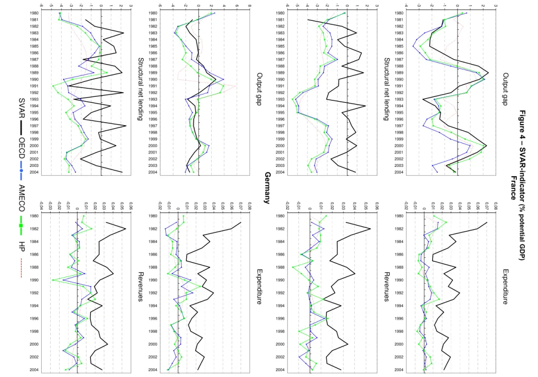
*). In Figure 4 (top left panel), we have repeated for comparison the output gaps of the European Commission, OECD and the

one obtained by applying a Hodrick-Prescott filter. There is a rather close correspondence

between these measures and our supply shock based gap for France and Germany. Given

that we have only used the OECD elasticities for distinguishing shocks with transitory effects

on output, this is all the more remarkable. The smooth gap for Portugal and Spain underlines

the importance of supply relative to demand shocks in both countries. This was expected

given the strong economic catch-up that both countries have experienced. We believe that

potential output tracked much closer actual output developments in these countries. The

15 _{We are certainly not the first study to document that European countries have not left automatic stabilisers to}

usual statistical filtering methods are not adequate to capture this trend behaviour. Cyclical

fluctuations are therefore rather minor. We provide some further robustness checks in the

Appendix 2.16

Overall, there was an improvement in economic conditions at the start of EMU in all

countries. We find that economic conditions have worsened in both France and Germany in

more recent years. We nevertheless find the crisis in Germany to have set in somewhat

earlier and to be more prolonged. As cyclical fluctuations are not large, we do not find much

economic slack in recent years in Spain or Portugal.

[INSERT FIGURE 4 HERE]

4.3. The fiscal indicator

We are now ready to discuss the indicator of discretionary fiscal stance. In general, the

measure is more volatile than the measures derived with conventional methods (see Figure

4, bottom left panel). In many instances, our measure leads the smoothed measures in the

direction of change. The fiscal indicator is usually smaller than conventional measures of the

cyclically adjusted deficit. This reflects the definition of the structural balance, by which we

take out the automatic stabilisers and the induced stabilisation effects caused by fiscal

policies. In addition, fiscal policy also affects permanent output and therefore the structural

fiscal position fluctuates around balance. The indicator is also much more volatile. This

follows from the major contribution of supply and fiscal shocks to the variation in output,

spending and revenues. One of the causes of this strong volatility – apart from the dominant

supply side shocks – is the procyclical bias that characterises fiscal policymaking. This

induces extra variation, especially so in government revenues.

We may expect the measure to coincide with some episodes of fiscal laxness or

retrenchment. In Table 5, we gather the fiscal years in which Alesina and Perotti (1997)

argue a strong expansion or adjustment to have occurred in these countries. For the sample

period that overlaps with their study (till 1995), the correspondence is indeed close.

Comparing the changes in Figure 4 (bottom left side) to the years in Table 5, we would

detect nearly always the same events. For Germany, the expansion that precedes

Reunification also shows up as a structural worsening of the deficit in our model. We only

have some problems in finding back the switches in Portuguese fiscal policy early eighties,

16

but would definitely have dated the expansion of 1987 and the ensuing consolidation of

1989. We pick out the French expansion of 1992 too, but see it as following on a string of

expansionary budgets.

Table 5. Large fiscal expansions and contractions Strong expansion Strong consolidation

France 1981,1992 -

Germany 1990 1989

Portugal 1981,1983, 1987 1980,1982,1984,1989

Spain 1982 1986,1987

Source: Alesina and Perotti (1997). Note: a strong expansion (adjustment) occurs if Blanchard’s Fiscal Impulse exceeds 1.5% (-1.5%) of GDP.

In Figure 4, we can see a substantial shift in discretionary policies towards structurally

positive net lending ratios in the period just before EMU. This is perhaps least visible in

Germany, but the initial conditions were probably not such as to urge a strong and prolonged

consolidation for reaching the Maastricht deficit limit. A substantial consolidation had already

taken place at the end of the eighties. In the other countries, the structural effort was more

drawn out. France started consolidation already in 1993, while it gathered pace in Portugal

and Spain only in 1995. This also confirms evidence in Fatás and Mihov (2003).

How has this consolidation been achieved? The right hand side panels of Figure 4 plot the

growth rates of structural expenditures and revenues. These reveal that structural

consolidations in the nineties have been based on a mixture of expenditure and revenue

measures. But the combination of adjustments in the policy instruments has changed over

time in a remarkably similar fashion in all countries. Initially, we see relatively moderate

expenditure growth and in some cases even relevant spending cuts (Germany and

Portugal). This strategy is reversed closer to the deadline of EMU. Tax increases start to

bear the largest burden for bringing down deficits. Given the urgency of qualifying for the

EMU criteria, taxes have seemingly been the easiest instrument to adjust. Notice the rather

close match between the VAR-measure of structural spending and revenues and the

(difference log of the) HP-trend on unadjusted total expenditure and revenues. The

measures of OECD and AMECO display slightly lower growth rates. This owes again to our

definition of the structural series. The efforts in reaching EMU led to the levelling off or even

moderate declines in debt ratios. A plot of the structural fiscal indicator to the debt ratio

shows how well the indicator captures these consolidations in debt (Appendix 2).

What went wrong then with the application of the Stability and Growth Pact in France,

countries. The increased tax revenues in the years prior to EMU led to a starting point of

structural surplus. The persistence in these tax rises improved actual balances thanks to the

favourable economic conditions at the time. But this has been exploited to increase

expenditures in a commensurate way. Especially in Portugal, the expansion in expenditures

seems to have held back an improvement in the structural position. The only exception here

is Spain that further brought down expenditure, even in the presence of strong revenue

increases. Simultaneously, the tax revenues that stream in during economic boom seem to

have been undone by decisions to bring down tax rates in most countries. This considerably

worsened the structural balance. As economic boom turned into bust again, the decline in

revenues led to a substantial worsening of actual balances, pushing the deficit beyond the

3% threshold. However, the revenue declines have hardly ever been matched by sufficient

cutbacks in government spending in the following years. Corrective measures in 2004 have

improved the structural deficit. But the measures are mainly taken on the revenue side

again, by undoing once more previous decisions to cut tax rates. To avoid further

infringement of the budget rules, the adjustment in Germany and France has taken place via

the route of tax rises during economic slack. This has once more reinforced the procyclical

bias in fiscal policy-making. This also highlights the mechanism by which spending gets

locked in, and causes a ‘ratcheting up’ in the size of government.

The overall situation seems less dramatic in Portugal, as revenue changes have been

supported by comparable spending decisions.17 For Spain, the moderate decline in tax

revenues in 2001 and 2002 was not entirely matched with spending cuts, leading to a slight

deterioration of the structural indicator. The expansionary measures taken in 2004 have led

to a breach of a balanced structural budget for the first time since 1995. Unsurprisingly, the

expansion of fiscal policies in all countries reflects itself in rising debt ratios in recent years

(see Appendix 2).

How useful is our indicator for assessing budgetary reform? We have argued above that

aggregate spending or revenue measures contribute to long-term growth. Its contribution

may perhaps be small relative to productivity rises in the private sector, and part of the effect

could be swamped due to procyclical policies that induce macroeconomic fluctuations (and

its consequent negative effects on growth). We do not believe this is the final word on the

contribution of fiscal policy. A more detailed analysis of different spending/tax items could

shed light on their specific growth enhancing effects.

17 _{One should notice that several one-off measures mask the true deterioration in the Portuguese or the Spanish}

4.4. Some sensitivity analysis

The results might be influenced by some particular parameter value that we have drawn

from the OECD in order to distinguish business cycle and fiscal demand shocks. There are

various reasons for considering these aggregate elasticities with some caution.

First, elasticities are assumed to be time-invariant. These are not representative of the tax

and spending structures that have prevailed in historical samples, however. In some

countries, the expansion of the welfare state has led to gradually larger tax bases and

dramatic changes in tax systems (Portugal and Spain). But even in France and Germany,

time-variation cannot be neglected. Budget elasticities tend to move over the business cycle

as well. Changes in elasticities also throw up a more subtle difficulty in the interpretation of

the fiscal shocks that we have already discussed in section 4.2. On the revenue side,

discrete policy changes involve decisions on the ratio of average to marginal tax rates and

the breadth of tax bases rather than on total amounts. Only if changes in total revenue

amounts coincide with these decisions, do we identify correctly shocks on the revenue side

of the budget. Second, given the difficulties in identifying all channels through which

changes in interest rates and inflation may impinge on various revenues and spending

categories, the OECD simply abstains from adjusting interest payments for cyclical variation

and assumes the net effect of inflation to be zero. This only reinforces the argument in

favour of our economic approach in which we specify a role for long-term and business cycle

fluctuations. However, our use of the OECD numbers can be argued to be inconsistent as

these have been derived under these methods. Finally, auxiliary assumptions on the various

parts of the calculation of budget elasticities may cumulate into quite some uncertainty in the

final estimates of elasticity.

Our first robustness check on the elasticity parameters illustrates the effects of this

uncertainty. Table 6 shows the wide range of net lending elasticity that is obtained by

varying only the elasticity of wages to output two standard errors below and above its point

estimate.18 We conduct a grid search on different values for

γ

and

α

that Girouard and André

(2005) provide. For all possible combinations of this revenue elasticity

α

and for a given

spending elasticity

γ

, we impose the identification scheme as in Table 2 on the VAR. For

any of the parameter values, we always find convergence to a result identical to that

18 _{The wage elasticity is used for calculating the elasticity of the income tax. See Girouard and André (2005) for}