BJRS
RADIATION SCIENCES
07-02A (2019) 01-16
ISSN: 2319-0612
Accept Submission 2018-10-31
EVALUATION OF ITERATIVE ALGORITHMS FOR
TOMOGRAPHY IMAGE RECONSTRUCTION
A. F. Velo
a; A. G. Alvarez
a; M. M. Hamada
a; C. H. Mesquita
aa Instituto de Pesquisas Energéticas e Nucleares- IPEN/CNEN-SP. 05508-000, São Paulo, São Paulo, Brasil
ABSTRACT
The greatest impact of the tomography technology currently occurs in medicine. The success is due to the fact that human body presents standardized dimensions with well-established composition. These conditions are not found in industrial objects. In industry, there is a great deal of interest in using the tomography in order to know the inner part of (i) manufactured industrial objects or (ii) the machines and their means of production. In these cases, the purpose of the tomography is: (a) to control the quality of the final product and (b) to optimize the production, contributing to the pilot phase of the projects and analyzing the quality of the means of production. This scan system is a non-destructive, efficient and fast method for providing sec-tional images of industrial objects and it is able to show the dynamic processes and the dispersion of the ma-terials structures within these objects. In this context, it is important that the reconstructed image may present a great spatial resolution with a satisfactory temporal resolution. Thus, the algorithm to reconstruct the imag-es has to meet thimag-ese requirements. This work consists in the analysis of three different iterative algorithm methods, namely the Maximum Likelihood Estimation Method (MLEM), the Maximum Likelihood Trans-mitted Method (MLTR) and the Simultaneous Iterative Reconstruction Method (SIRT. The analyses in-volved the measurement of the contrast to noise ratio (CNR), the root mean square error (RMSE) and the Modulation Transfer Function (MTF),in order to know which algorithm fits the conditions to optimize the system better.
The algorithms and the image quality analyses were performed by Matlab® 2013b.
1. INTRODUCTION
Unlike the standard aspect of the computed tomography (CT) for medical application, industrial tomography systems applications should be adapted to the different size and geometry objects, usually placed in an ag-gressive environment, which contains flammable superheated or corrosive materials, and, eventually, subject to high internal pressure, all these factors bring in many difficulties for setting CT devices [1, 2]. In addition, the industrial systems involve multiphase dynamic processes containing solids, liquids and gases mixtures [3-7]. In other words, it is necessary to develop a tomographic system suitable for each industrial purpose [2, 6].
The CT systems based on transmission uses an array of encapsulated radioactive sources and detectors placed in opposite sides of the targeted object [7-9]. First generation tomography systems consist of a source emitting a collimated radiation pencil beam and a radiation detector (Fig.1a). The source-detector system moves in opposite sides of the object, measuring the attenuation of radiation at each position [10].
In the second generation CT systems, a set of detectors is placed opposite to the radioactive source with fan beam, moving (source and detector) around the object under study (Fig.1b) [10].
In the tomography of third generation, the source is collimated so that the path crossed by beams is similar to a fan (Fig.1c). The system rotates around the targeted object, obtaining a particular view for an "x" position of the source-detector array. In this type of system, several sources and arrays of multiple detectors may be used [10].
Finally, the so-called fourth-generation CT systems use a fixed array of detectors (a large number of detec-tors mounted on a fixed ring) and a radioactive source that rotates around the object (Fig.1d). Records of any measure are from the detector, representing a view of the object. However, all CTs are constituted, basically, of the same parts: radioactive sources; radiation detectors; a data acquisition system and a suitable computer [10].
Figure 1: (A) translation - rotation of a pencil beam (first generation), (B) translation - rotation of sources
in a fan beam (second generation), (C) rotation of a fan-beam (third generation), (D) detector fixed - rota-tion source (fourth generarota-tion).
These scan systems are able to show the dynamic processes and the dispersion of the material structures within the objects. In this context, it is important that the tomography reconstructed image may present a great spatial resolution with a satisfactory temporal resolution [11, 12]. Thus, the algorithm selected to re-construct the images has to meet these requirements. The aim of this work consists in the analysis of differ-ent iterative algorithms.
2. MATERIALS AND METHODS
A third generation computed tomography system, comprising three NaI(Tl) detectors of 50 x 50 mm2
(di-ameter, thickness) shielded with lead, was used. The detectors were placed on a gantry in fan-beam geometry opposite to the gamma ray source, as shown in Fig.1. The three NaI(Tl) detectors were individually collimat-ed with lead containing a septa of 2 x 5 x 50 mm3 (width, height, depth). The detectors move 53 times in a
step angle of 0.226 degrees, emulating 159 detectors per projection. The counting time for sampling was 5 seconds. Thereafter, the support table containing the gantry and the 137Cs gamma source (Fig. 1) rotates six
degrees forward and this process goes on up to completing 360 degrees, totalizing 60 projections. For a total of 9540 samples (159 'virtual detectors' x 60 projections), the system spends 15,900 seconds or 4.4 hours to obtain each tomography image. The 137Cs radioactive source, with an activity of 3.0 GBq (81 mCi), was
placed into a radioactive shield-case with an aperture angle of 36 degrees (Fig. 2). This system had been previously described by Mesquita et al [12, 13].
Figure 2: Diagram of the third generation CT scanner used. (a) top view and (b) side view [14]
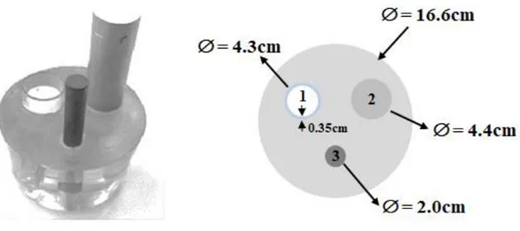
A multiphase phantom was used to evaluate the performance of the multisource third generation tomography device [12]. The phantom consists of a polymethylmethacrylate (PMMA ((ρ ≈ 1.19 g/cm3)) solid cylinder
containing three holes: one filled with steel (ρ ≈ 7.874 g/cm3), another with aluminum (ρ ≈ 2.698 g/cm3) and a third one empty (filled with air) and surrounded with glass, as illustrated in Fig. 3.
Figure 3: Illustration of the multiphase phantom; (1) Air surrounded with glass wall; (2) aluminum bar;
and (3) steel bar. The phantom is composed of PMMA.
The image reconstruction is based on the exponential decay law defined by equation (1), which is known as Lambert-Beer’s law [15]:
𝐼 = 𝐼0𝑒− ∑ 𝜇𝑖𝑤𝑖,𝑗⃗
𝑁
𝑖=1 (1)
where 𝐼0 is the initial intensity of the beam radiation that focuses on the object at j direction, 𝐼 is the intensity of the beam radiation through the object, N is the number of pixels on the matrix, µ𝑖 is the linear attenuation coefficient of the matter and 𝑤𝑖,𝑗 is the length of the beam radiation through pixel I and it is an element of the weighted matrix W [15]. Fig. 4 illustrates the scheme of the discretized grip to measure 𝑤𝑖,𝑗 .
Figure 4: Discretized grid
The discretized ray sum for each ray j (j = 1, 2, …, J) may be expressed as the equation (2) [15].
𝑝𝑗𝑛𝑜𝑟𝑚𝑎𝑙𝑖𝑧𝑒𝑑= 𝑙𝑛 (𝐼𝑜𝑗 𝐼𝑗 ) = ∑ 𝑤𝑖𝑗𝜇𝑖 𝑁 𝑖=1 (2)
The size of W is defined by the number of pixels in the reconstruction grid. Due to Poisson noise corruption of the measured data, a term 𝜂𝑗 describing the noise is added to the equation (3) [15]:
𝑝𝑗𝑛𝑜𝑟𝑚𝑎𝑙𝑖𝑧𝑒𝑑 = 𝑙𝑛 ( 𝐼𝑜𝑗 𝐼𝑗 ) = ∑ 𝑤𝑖𝑗𝑥𝑖+ 𝜂𝑗 𝑁 𝑖=1 (3)
Solving a high number of linear equations, based on measurements corrupted by random variables and noise, requires the use of iterative algorithms. The iterative methods are divided in two categories, the algebraic and the statistical methods [15]. Algebraic reconstruction methods solve a set of linear equations by comparing the measured data set to an estimate and reducing the difference between them. Statistical methods recon-struct the image by implementing the maximization of the likelihood function, recognizing Poisson distribu-tion funcdistribu-tion of the projecdistribu-tions in reladistribu-tion with the measurements [15]. In the present work, the Simultaneous Iterative Reconstruction Technique (SIRT), the Maximum Likelihood Expectation Maximization (MLEM)
and the Maximum Likelihood Algorithm for Transmission Tomography (MLTR) were used to
recon-struct the images, so that the first algorithm is an algebraic method and the last two are statistical
methods.
The SIRT algebraic method is expressed by the equation (4) [15]
µ
𝑗(𝑛+1)= µ
𝑗𝑛+ 𝛿 ∑ 𝑤
𝑖𝑗(𝑔
𝑖− ∑
𝑁𝑘=1𝑤
𝑖𝑘µ
𝑘 (𝑛))
∑
𝑁𝑤
𝑗𝑘2 𝑘=1 𝑀 𝑖=1(4)
where, µ is the pixel index, 𝛿 is the relaxation parameter, 𝑔 is the 𝑃
𝑛𝑜𝑟𝑚𝑎𝑙𝑖𝑧𝑒𝑑and w is the weighted
matrix element.
The statistical methods, MLTR and MLEM, are expressed by equations (5) and (6), respectively
[15].
µ
𝑗(𝑛+1)= µ
𝑗(𝑛)+
∑
(𝑤
𝑖𝑗(𝐼
0𝑒
(− ∑ ℎ𝑖𝑘µ𝑘 (𝑛) 𝑁 𝑘=1 )− 𝐼))
𝑀 𝑖=1∑
(𝑤
𝑖𝑗𝐼
0𝑒
(− ∑ 𝑤𝑖𝑘µ𝑘 (𝑛) 𝑁 𝑘=1 )∑
𝑤
𝑖𝑘 𝑁 𝑘=1)
𝑀 𝑖=1(5)
µ
𝑗(𝑛+1)=
∑
[𝐼
0𝑒
(− ∑ 𝑤𝑖𝑘µ𝑘 (𝑛) 𝑁 𝑘=1 )(1 − 𝑒
−𝑤𝑖𝑗µ𝑗 (𝑛))]
𝑀 𝑖=1∑
[𝐼
𝑖− 𝐼
̅ + 0.5(1 + 𝑒
𝑖 −𝑤𝑖𝑗µ𝑗(𝑛))𝐼
0𝑒
(− ∑ 𝑤𝑖𝑘µ𝑘 (𝑛) 𝑁 𝑘=1 )]
𝑀 𝑖=1(6)
All reconstruction was performed in a matrix of 128x128 pixels and 200 iterations. All physical
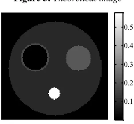
measurements and reconstructions were performed by Matlab 2013b®. Root Mean Square Error
(RMSE) was measured to evaluate which iterative algorithm approaches the pixel values, obtained
experimentally for the theoretical values. This method is widely used to measure the quality of the
image. The RMSE was obtained by equation (7) [16],
𝑅𝑀𝑆𝐸 = √
∑
(𝜇
𝑖− 𝜇
̂ )
𝑖 2 𝑁𝑖=1
where, 𝜇
𝑖is the experimental pixel value obtained, 𝜇
̂ is the theoretical linear attenuation coefficient.
𝑖The theoretical image is presented in Fig. 5.
Figure 5: Theoretical image
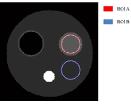
The Contrast to Noise Ratio (CNR) was measured selecting regions of interest (ROIs) in the images of the phantom (Fig. 2) obtained, experimentally, for the different algorithms. A circular ROI was placed over the cylinder corresponding to the aluminum (ROI A) and another ROI, with the same size of ROI A, placed over the background, corresponding to the PMMA (ROI B), then the values of the CNR were obtained by equa-tion (8) [16,17 ].
𝐶𝑁𝑅 = |𝜇̅̅̅ − 𝜇𝐴 ̅̅̅̅|𝐵 √𝜎𝐴2+ 𝜎𝐵2
2
(8)
where, 𝜇̅̅̅ is the mean pixel value of ROI A, 𝜇𝐴 ̅̅̅̅ is the mean pixel value of ROI B, 𝜎𝐵 𝐴is the standard devia-tion of ROI A and 𝜎𝐵 is the standard deviation of ROI B. The ROIs are presented in Fig. 6, where the red circle represents ROI A and the blue circle represents ROI B.
0.1 0.2 0.3 0.4 0.5
Figure 6: ROIs used to measure the CNR
The most comprehensive metric method used to measure and report spatial resolution of imaging systems is the modulation transfer function (MTF) [17-20]. Conventionally, the spatial resolution is estimated as the inverse of the value at 10% of MTF curve [17-20]. In the present work, the MTF was calculated using the Edge Spread Function, commonly known as ESF parameter [19, 20].
3.
RESULTS AND DISCUSSIONThe reconstructed images of the phantom obtained by the third generation industrial tomography are present-ed in Fig. 7, where Fig. 7a. represents the reconstruction by SIRT algorithm; Fig. 7b., by MLTR algorithm; and Fig. 7c., by MLEM algorithm.
Figure 7: Images reconstructed of the phatom using (a) SIRT algorithm; (b) MLTR algorithm and (c). MLEM
algorithm
RMSE parameter, applied to perform the quality of the image for the three different algorithms (SIRT, MLTR and MLEM), was calculated using equation (7), comparing the experimental images with the theoret-ical image. Fig. 8 shows the curve behavior for each algorithm.
Figure 8: RMSE analysis for the three algorithms
Fig 8 shows that the MLEM algorithm converges and approaches the theoretical values with fewer numbers of iteration compared to the other two algorithms. By this analysis, it is possible to observe that the images
100 101 102 10-1 Iteration number R M SE ( ) SIRT MLTR MLEM
reconstructed by MLEM algorithm present better quality, converging their optimum with fewer numbers of iteration.
The analysis of the noise influence was performed by CNR parameter on the three different algorithms. The results are shown by Fig. 9. From this figure, it is possible to observe that even MLEM and MLTR algo-rithms reaching a higher CNR value in the first iterations, these values decrease as the number of iterations rises, different from SIRT algorithm, which reaches a lower CNR value, but decreases less than the others, what means that the noise influences less in the images reconstructed by the SIRT algorithm, as the number of iteration increases, when compared to the other two algorithms.
Figure 9: CNR analysis by the number of iterations
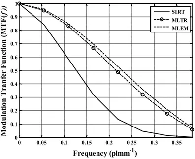
The spatial resolution of the reconstructed images was measured by the MTF (f). MTF curves, by the fre-quency spectrum (plmm-1) of the three algorithms, at the iteration number of 200, are presented in Fig. 10.
0 50 100 150 200 0 2 4 6 8 10 12 14 Iteration number C on tr as t to N oi se R at io (C N R ) SIRT MLTR MLEM
Figure 10: MTF (f) of the three different algorithms, at the iterative number of 200
From Fig. 10, the MLEM algorithm presents a better spatial resolution in all the frequency spectra,
compared to the other algorithms. The maximum spatial resolution of the system is measured at
10% of the MTF; in other words, the spatial resolution is calculated by the inverse of the frequency
in 10% of the MTF. Thereby, the resolution for SIRT, MLTR and MLEM is about 2.86 mm, 2.75
mm and 2.70 mm, respectively.
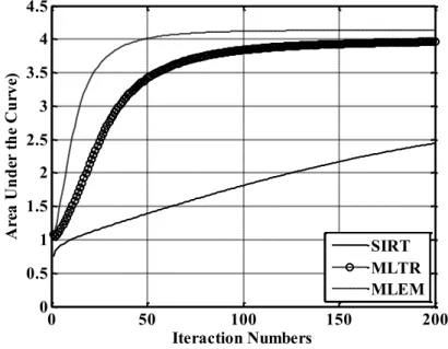
Fig. 11 shows the area under the curve of the MTFs obtained for all iterative number of the three
algorithms.
0 0.05 0.1 0.15 0.2 0.25 0.3 0.35 0 0.1 0.2 0.3 0.4 0.5 0.6 0.7 0.8 0.9 1 Frequency (plmm-1) M od u la ti on T ra n fe r F u n ct io n ( M T F ( f )) SIRT MLTR MLEMFigure 11: Area under the curve of the MTFs by the number of iterations
Fig. 11 shows that MLEM presents a better spatial resolution for all iterative numbers compared with the other algorithms. It is possible to observe, as well, that for the MLEM and the MLTR around 100 iterations, the spatial resolution reaches its optimum value and it maintains constant as the iteration numbers rises. This fact suggests that, for these two algorithms, the iterations could stop at 100, where the spatial resolution reached a higher value, reducing the time of reconstruction and avoiding the growth of noise, as observed in figure 9.
4.
CONCLUSIONThe results of RMSE values showed that the MLEM algorithm converges and approaches to the theoretical values with a lower number of iterations, compared to the other two algorithms, evidencing that this algo-rithm has a better image quality.
The CNR analysis showed that MLEM and MLTR algorithms reach a higher CNR value, but the number of iterations does not rise as the same, due to the growth of noise, different from the SIRT algorithm, that reaches a lower CNR value, but it decreases less than the others, what means that the noise has less influence on the images reconstructed by the SIRT algorithm than those by the other two algorithms.
The spatial resolution value obtained with SIRT, MLTR and MLEM algorithms is 2.86 mm, 2.75 mm and 2.70 mm, respectively, which means that the MLEM has a better spatial resolution.
0 50 100 150 200 0 0.5 1 1.5 2 2.5 3 3.5 4 4.5 Iteraction Numbers A re a U n d er t h e C u rv e) SIRT MLTR MLEM
The area under the curve of the MTFs for all number of iterations showed that at around 100 iterations, the spatial resolution for MLTR and MLEM reaches its optimum value, which means that for these two algo-rithms the iterations could stop at this value reducing time of reconstructing and avoiding the growth of noise. The SIRT algorithm has worse spatial resolution, and did not get its optimum value, suggesting that this algorithm has to keep iteration until reaches the optimum value.
For all the analysis measured, the MLEM showed to be a better algorithm to be applied on the systems of the third generation industrial tomography.
5.
ACKNOWLEDGMENTThe authors express their acknowledgment to CNEN, FAPESP and the IAEA for the financial support. The authors, Carlos Henrique de Mesquita and Margarida Mizue Hamada, thank CNPq and Alexandre França Velo thanks CNEN, for their fellowship.
![Figure 2: Diagram of the third generation CT scanner used. (a) top view and (b) side view [14]](https://thumb-eu.123doks.com/thumbv2/123dok_br/18283626.881970/4.892.117.770.622.985/figure-diagram-generation-ct-scanner-used-view-view.webp)