https://doi.org/10.5194/bg-14-2955-2017 © Author(s) 2017. This work is distributed under the Creative Commons Attribution 3.0 License.
Biological and environmental rhythms in (dark) deep-sea
hydrothermal ecosystems
Daphne Cuvelier1,a, Pierre Legendre2, Agathe Laës-Huon3, Pierre-Marie Sarradin1, and Jozée Sarrazin1 1Ifremer, Centre de Bretagne, REM/EEP, Laboratoire Environnement Profond, Plouzané, 29280, France
2Département de Sciences Biologiques, Université de Montréal, P.O. Box 6128, Succursale Centre-ville, Montréal, H3C 3J7, Québec, Canada
3Ifremer, Centre de Bretagne, REM/RDT, Laboratoire Détection, Capteurs et Mesures, Plouzané, 29280, France acurrent address: Mare – Marine and Environmental Sciences Centre, Department of Oceanography and Fisheries, Rua Professor Frederico Machado 4, Horta, 9901-862, Portugal
Correspondence to:Daphne Cuvelier ([email protected]) Received: 3 November 2016 – Discussion started: 8 November 2016 Revised: 10 April 2017 – Accepted: 4 May 2017 – Published: 20 June 2017
Abstract. During 2011, two deep-sea observatories focusing on hydrothermal vent ecology were up and running in the At-lantic (Eiffel Tower, Lucky Strike vent field) and the North-east Pacific Ocean (NEP) (Grotto, Main Endeavour Field). Both ecological modules recorded imagery and environmen-tal variables jointly for a time span of 23 days (7–30 October 2011) and environmental variables for up to 9 months (Octo-ber 2011–June 2012). Community dynamics were assessed based on imagery analysis and rhythms in temporal variation for both fauna and environment were revealed. Tidal rhythms were found to be at play in the two settings and were most visible in temperature and tubeworm appearances (at NEP). A ∼ 6 h lag in tidal rhythm occurrence was observed be-tween Pacific and Atlantic hydrothermal vents, which corre-sponds to the geographical distance and time delay between the two sites.
1 Introduction
All over our planet, animals are influenced by day and night cycles. Entrainment occurs when rhythmic physiological or behavioural events in animals match the periods and phase of an environmental oscillation, e.g. circadian rhythms, to light–dark cycles. In marine populations such cycles are ev-ident in the photic zone (Naylor, 1985). However, more re-cently similar cycles have become apparent in deep-sea or-ganisms and populations as well, at depths where light does
not penetrate. At these greater depths, fluctuations in light in-tensity are likely to be replaced by changes in hydrodynamic conditions (Aguzzi et al., 2010). Several studies reveal the presence of tidal cycles in environmental variables (such as currents, fluid emission, temperature) in the deep sea, partic-ularly in hydrothermal vents (e.g. Tivey et al., 2002; Thom-sen et al., 2012; Barreyre et al., 2014; Sarrazin et al., 2014; Lelièvre et al., 2017) and the influence of tides on the deep-sea organisms has been previously inferred. Additionally, an actual tidal rhythm has been revealed in visible faunal den-sities and appearance rate for inhabitants of various deep-sea chemosynthetic environments – e.g. a semi-diurnal tidal component in buccinids at cold seeps (Aguzzi et al., 2010) and semi-diurnal and diurnal tidal components in siboglin-ids at vents (Tunnicliffe et al., 1990; Cuvelier et al., 2014). Presumably, though difficult to statistically demonstrate, the deep-sea organisms respond to or reflect the changing sur-rounding environmental conditions, which are modulated by hydrodynamic processes including the tides.
Despite the growing realisation that tidal influences are in-deed at play in the deep ocean, it remains hard to actually re-veal these patterns because of the isolation of the ecosystem and the limited access to the longer time series. The use of deep-sea observatories, which have been deployed recently in various seas and oceans (see Puillat et al., 2012 for an overview), brings new insights into the dynamics of these remote habitats. First ecological analyses based on deep-sea observatories have been published (Juniper et al., 2013;
Matabos et al., 2014, 2015; Cuvelier et al., 2014; Sarrazin et al., 2014; Lelièvre et al., 2017), and many more works are in progress.
The current observatory-based study allows a unique com-parison of hydrothermal vent community dynamics between two different oceans featuring a different seafloor spread-ing rate. Data originatspread-ing from the deep-sea observatories MoMAR, now EMSO-Azores, on the slow-spreading Mid-Atlantic Ridge (MAR) and NEPTUNE, now called Ocean Networks Canada (ONC), on the faster-spreading Juan de Fuca Ridge (Northeast Pacific, NEP), featuring the same time span and resolution, have been analysed. The two oceans are characterised by different vent fauna, with a visual predomi-nance of Bathymodiolus mussels in the shallower (< 2300 m) Atlantic and Ridgeia tubeworms in the NEP, but they do share higher taxonomic groups. Following key questions are put forward: (i) Are there rhythms discernible in both hydrother-mal settings? (ii) Is there a lag/time difference in community dynamics and environmental variables observed between the two oceans? (iii) Which environmental variables influence community dynamics? And, finally, (iv) do the shared taxa occupy similar microhabitats and possible niches in each ocean? Answering these questions will provide new insights in understanding local vent community dynamics and will enlighten us on similarities and differences between oceanic ridges and oceans. In order to do this, a dual approach was wielded, assessing a short-term comparison between fauna and environment (23 days) and a longer-term comparison of environmental variables (9 months) featuring the same ob-servation window at both study sites.
2 Material and methods
2.1 Observatories and study sites
Two similar ecological observatory modules, called TEMPO and TEMPO-mini, were deployed in two different oceans in 2011 (Fig. 1). The first one (TEMPO) was part of the EMSO-Azores observatory (http://www.emso-fr.org/ EMSO-Azores) and was deployed at the Lucky Strike vent field on the MAR, south of the Azores. The wireless EMSO-Azores observatory consists of two main hubs, positioned east and west of the central lava lake that is characteristic of the Lucky Strike vent field. The eastern hub (SeaMoN East; Blandin et al., 2010) focuses on hydrothermal vent ecology and hosts the TEMPO module. TEMPO 2011 was positioned at 1694 m depth at the southern base of a large 11 m high hy-drothermally active edifice called Eiffel Tower. Its counter-part, TEMPO-mini, was implemented on the region-scaled cabled network NEPTUNE (http://www.oceannetworks.ca/) in the NEP, as part of the Endeavour instrument node. It was deployed at a depth of 2168 m on a small 5 m high platform on the north slope of the Grotto hydrothermal vent, a 10 m high active edifice at Main Endeavour Field (MEF). Both
modules were equipped with a video camera (Axis Q1755), temperature probes, a CHEMINI Fe analyser (Vuillemin et al., 2009) and an optode measuring temperature and oxygen. An additional instrument measuring turbidity was deployed in the vicinity of the TEMPO module in 2011 (Table 1). The biggest discrepancy between both modules was the energy provision, with the Atlantic one (TEMPO) being autonomous and battery dependent (wireless) and the NEP one (TEMPO-mini) being connected to a cabled network. Detailed descrip-tions of both modules can be found in Sarrazin et al. (2007, 2014) for TEMPO and Auffret et al. (2009) and Cuvelier et al. (2014) for TEMPO-mini.
Henceforth, the Atlantic set-up (TEMPO on MoMAR/EMSO-Azores) will be referred to as MAR and the Pacific set-up (TEMPO-mini on NEPTUNE/ONC) set-up as NEP (Fig. 1).
2.2 Data collection and recordings
Data collected consisted of video imagery recordings, tem-perature measurements, iron and oxygen concentrations, and turbidity measurements (the latter for MAR only) (Table 1; Cannat et al., 2015 for MAR), which were recorded jointly for the period 7–30 October 2011. Differences in recording resolutions were mainly due to different observatory set-ups and more particularly due to the cabled or wireless network characteristics and their inherent energy limitations (contin-uous power vs. battery dependence). Lights were powered on with the same frequency as the imagery recording (ev-ery 6 h) at MAR, contrastingly to NEP where lights were on continuously during the period analysed (23 days). At NEP, TEMPO-mini was equipped with a thermistor array in which two probes (T602 and T603) were deployed on an assemblage most similar to the one filmed (see Cuvelier et al., 2014). Therefore, only those two probes were used in the comparison to the MAR temperature data, which were recorded directly on the filmed assemblage.
Iron (from here on referred to as Fe) concentrations were measured on top of the assemblage and within the field of view (FOV) at MAR (Laës-Huon et al., 2015; Sarradin et al., 2015) and below the FOV at NEP. An in situ calibra-tion was performed at NEP, analysing two Fe standards a day of 20 and 60 µmol L−1; no such calibration took place at MAR. At NEP, sampling frequency was changed from twice (30 September–18 October 2011) to once a day (19 October 2011–31 January 2012) due to rapidly decreasing reagents. Fe concentrations were analysed over a longer term and used to explore the differences between the observatory settings.
Closer examination of data recorded by the optode re-vealed some inconsistencies between the measured temper-ature and the O2 concentrations. As the O2 concentrations were corrected by the temperature, a difference in the re-sponse time between the temperature and oxygen sensor within the same instrument was presumed. This lag could not be quantified, making comparisons with other
observa-Table 1. Overview of the location, data recorded and the recording resolutions of all variables of the two observatories on the NEP and MAR.
TEMPO MoMAR/EMSO-Azores (MAR) TEMPO-mini NEPTUNE (NEP) Energy provision Batteries (wireless) Cabled
Coordinates lat 37◦17.33210N 47◦56.95740N Coordinates long 32◦16.53340W 129◦05.89980W
Depth 1694 m 2168 m
Imagery 4 min every 6 h (at 00:00, 06:00, 12:00, 18:00 UTC) Continuous for ∼ 23 days followed by 30 min every 4 h (at 02:00, 06:00, 10:00, 14:00, 18:00 , 22:00 UTC) Temperature One measurement every 5 min One measurement every 30 s
Optode (oxygen + temperature)∗ One measurement every 15 min One measurement every 15 min CHEMINI Fe Twice a day Twice a day/daily
Turbidity (NTU) One measurement every 15 min NA
∗Limited usefulness due to issues related to correctly calculate the oxygen concentrations. NA stands for not available.
Figure 1. Location of the two study sites in the Atlantic and the Pacific oceans, along with some other well-known vent fields for reference purposes. The NEP inset (top) shows the location of the different instrumented nodes of Ocean Networks Canada on the right and the TEMPO-mini ecological module deployed at Main Endeavour Field on the Juan de Fuca Ridge on the left. The MAR inset (bottom) represents a sketch of the Atlantic observatory (EMSO-Azores) at Lucky Strike vent field on the left and the TEMPO ecological module on the right. For more details of the exact location of the observatories within the hydrothermal vent fields see Matabos et al. (2015) for MAR and Cuvelier et al. (2014) for NEP.
tions impossible. Oxygen concentrations measured were thus merely used as illustration to compare the differences be-tween the two hydrothermal settings.
Turbidity was only measured at the MAR observatory in nephelometric turbidity units (NTU), which were straight-forward in their interpretation; i.e. the higher they were, the more turbid. The sensor was not calibrated as such since its response depended on the particle size, which was unknown.
Hence it only provided information on the relative turbidity (and peaks) of the environment.
2.3 Short-term temporal analyses
A unique subset of comparable data, allowing a joint assess-ment of fauna and environassess-ment, was available for the time period 7–30 October 2011 for both observatories. The im-age analysis period was limited because of data availability,
which in this case was restricted by the imagery recordings from NEP (see Cuvelier et al., 2014).
2.3.1 Imagery analysis
The variations occurring in the faunal assemblages in the two hydrothermal vent settings were analysed for 23 days. For this period, a screen still was taken every 6 h at 00:00, 06:00, 12:00 and 18:00 UTC. For each site, these screen stills were used as a template in Photoshop© to map and count faunal abundances. Faunal densities were quantified at a 6 h frequency, while the microbial coverage was assessed every 12 h. To pursue the latter, the microbial cover was marked in white and the rest of the image rendered in black. Us-ing the “magic wand tool” of the ImageJ image analysis software (Rasband, 2012), the surface covered by microor-ganisms was quantified and converted to percentages. Due to gaps in the data recordings different numbers of images were analysed for MAR and NEP (Table 2). These gaps were failed recordings (due to observatory black-out or instrument failure) or unusable video sequences (empty files, black or unfocused videos).
The surface filmed by each observatory was different (Ta-ble 2), which is why densities (individuals m−2)were used instead of abundances. In each setting, there was also a dis-crepancy between the surface filmed and that analysed (Ta-ble 2, Fig. 2). Some surfaces were not taken into account because of their increased distance to the camera, the focal point and associated light emission (referred to as “back-ground”) or due to the probe positioning within the FOV, making it impossible to quantify the fauna. These surfaces were marked in black and white on the map in Fig. 2 and were not included in the analysed surface calculations. Both maps were made based on a composed image, i.e. a merge of all images analysed, hence showing the most re-current species distributions. For MAR, main shrimp clus-ter/distribution was confirmed using Matabos et al. (2015). For NEP, heat maps from Cuvelier et al. (2014) were used to confirm and localise mobile fauna. This did not mean that the mobile fauna did not venture elsewhere, but it showed an average distribution.
The Atlantic and Pacific oceans feature distinct hydrother-mal vent fauna and, while they do share several higher-level taxa, most species are different for the two oceans (Figs. 1 and 2). The main visible species and engineering taxon present for the “shallower” (< 2300 m) mid-Atlantic vents is a mytilid (Bathymodiolus azoricus) versus a si-boglinid tubeworm for the NEP (Ridgeia piscesae). The sec-ond most characteristic Atlantic taxon is the Mirocaris for-tunata alvinocaridid shrimp (Desbruyères et al., 2001; Cu-velier et al., 2009). Contrastingly, no hydrothermal shrimp are present at NEP vents, but associated visible fauna con-sisted of Buccinidae (Gastropoda), Polynoidae (Polychaeta) and Pycnogonida (containing the family Ammotheidae) (Cu-velier et al., 2014; Table 2, Fig. 2). The latter two taxa are also
present at the shallower MAR sites but in lower abundances and represented by different genera and species, as well as a bucciniform gastropod (Turridae family). In the Atlantic FOV, a small patch of anemones (Actiniaria) was visible be-low the probe as well as single occurrences of Ophiuroidea. Visiting fish species consisted of Cataetyx laticeps (Bythiti-dae) and Pachycara sp. (Zoarci(Bythiti-dae) at MAR and NEP respec-tively. Segonzacia mesatlantica (Bythograeidae) crabs were abundant at MAR while Majid spider crabs could be occa-sionally observed at NEP.
Overall, imagery analysis was limited to the density as-sessment of the visible species (Cuvelier et al., 2012). In this perspective, tubeworm densities corresponded to the num-ber of visible tubeworms, i.e. those that had their branchial plumes out of their tube at the moment of the image analysis. From here on, tubeworms visibly outside of their tubes will be referred to as tubeworm densities. Stacked limpets were visible on the NEP imagery but were impossible to assess quantitatively due to their small size and piling (Cuvelier et al., 2014).
2.3.2 Environmental data
An active fluid exit was visible on the images of the MAR but not on the NEP recordings. The probe measuring the MAR environmental variables was positioned next to this fluid exit in the FOV, whilst the different probes of NEP (mul-tiple probes measuring different environmental variables; see in situ observatory set-up in Cuvelier et al., 2014) were de-ployed below the FOV. The frequencies with which the en-vironmental variables were recorded were listed in Table 1. Due to the large variability and steep gradients in environ-mental conditions observed in the hydrothermal vent ecosys-tems, the temperature variables used in the analyses were av-eraged per hour to reduce noise and variance. Only probes T602–T603 from NEP were used for comparison with MAR. The R package hydroTSM (Zambrano-Bigiarini, 2012) was used to create an overview of the variations of hourly tem-perature values during imagery duration. For those variables used as explanatory variable (temperature and turbidity) in the joint analyses with the available faunal densities, every 6-hourly value was taken (corresponding with the 6 h frequency at 00:00, 06:00, 12:00 and 18:00 UTC). Fe was only sampled with a 12 or 24 h frequency, hence limiting its use as an ex-planatory variable for the higher-resolution faunal dynamics. 2.3.3 Statistical analyses
Multivariate regression trees (MRTs; De’Ath, 2002) were computed on Hellinger-transformed faunal densities. This analysis is a partitioning method of the species density ma-trix of each observatory, constrained by time. It grouped consistent temporal observations and thus identified groups with similar faunal composition that were adjacent in time; these groups are called “temporal split groups” from here on.
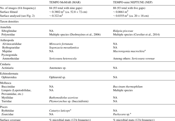
Table 2. Overview of the characteristics of the images analysed such as surface covered and taxa assessed within the FOV. The analysed surface on the MAR is about 10 times larger than that on the NEP. Gaps are failed or unusable video recordings.
TEMPO MoMAR (MAR) TEMPO-mini NEPTUNE (NEP) No. of images (6 h frequency) 84 (93 total with nine gaps) 88 (93 total with five gaps) Surface filmed ∼0.3802 m2(ca. 52.8 × 72 cm) ∼0.0661 m2
Surface analysed (see Fig. 2) ∼0.322 m2 ∼0.0355 m2(ca. 20 × 18 cm) Taxon densities
Annelida
Siboglinidae NA Ridgeia piscesae
Polynoidae Multiple species (Desbruyères et al., 2006) Multiple species (Cuvelier et al., 2014) Arthropoda
Alvinocarididae Mirocaris fortunata NA Bythograeidae Segonzacia mesatlantica NA
Majidae NA Macroregonia macrochira∗ Pycnogonida
Ammotheidae Sericosura heteroscela Among others: Sericosura verenae Cnidaria
Actiniaria Anemones sp. NA
Echinodermata
Ophiuroidea Ophiuroid sp. NA Mollusca
Buccinidae NA Buccinum thermophilum Limpets (Lepetodrilidae, NA Multiple species Provannidae, etc.)
Mytilidae Bathymodiolus azoricus NA Turridae Phymorynchussp. (bucciniform) NA Pisces
Bythitidae Cataetyx laticeps∗ NA
Zoarcidae NA Pachycarasp.∗
Surface coverage % microbial mats (12 h frequency) % microbial mats (12 h frequency)
∗
Visiting predators. NA stands for not available.
Each split was chosen to maximise the among-group sum of squares and the number of split groups was decided upon by choosing the tree with the lowest cross-validation error; that tree had the best predictive power. For this type of analysis, the observations did not need to be equispaced, as long as the constraining variable reflects the sampling time (Legen-dre and Legen(Legen-dre, 2012). The MRT partition was then sub-jected to a search for indicator taxa (IndVal analysis, Dufrêne and Legendre, 1997; multipatt function in R package Indic-species, De Caceres and Legendre, 2009). The IndVal index combined a measure of taxon specificity with a measure of fidelity to a group and thus revealed which taxon was signif-icantly more or less abundant in the group before than after the split. Its significance was assessed a posteriori through a permutation test (Borcard et al., 2011). The observed tem-porally consistent groups were delineated by colour codes within a redundancy analysis (RDA) ordination plot; RDAs were carried out on the Hellinger-transformed faunal den-sities and environmental variables to visualise the possible influence of the environmental constraints on the temporal groups found in the faunal density matrices. Environmental
variables were subject to forward selection (packfor pack-age in R; Dray, 2009), revealing those explaining most of the variation in faunal densities (α = 5 %).
Rhythms and periodicities in faunal densities and environ-mental variables were examined with Whittaker–Robinson (WR) periodograms (Legendre, 2012). These WR peri-odograms were computed on the faunal densities, with a 6 h resolution, and on the environmental variables with an hourly resolution. Prior to these analyses, stationarity was imple-mented by detrending time series when necessary. Time se-ries were folded into Buys Ballot tables with periods of 2 to a maximum of n/2 observations. The WR amplitude statis-tic was the standard deviation of the means of the columns of the Buys Ballot table. Missing values were taken into account and filled in by NA values (“not available”).
In order to establish differences or similarities in the vari-ations observed in temperature data from MAR and NEP, cross correlations were carried out on the hourly tempera-ture data for imagery duration (n = 553). Cross correlations could not be carried out between faunal and environmental variables because the time series were relatively short and
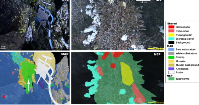
Figure 2. Sample image recorded by the ecological observatory modules for MAR and NEP (top) and a map of the fields of view (FOV) featuring the various taxa assessed (bottom). Taxa or other features that are shared between the two observatories share the same colour codes. Gastropoda applies to Buccinidae for NEP and bucciniform Turridae on MAR. White substratum is possibly anhydrite with encrusted microbial mats. “Mussel background”, “background” and “probe” were areas that were not assessed. The white arrow represents the fluid flow exit and direction. No visible emission was observed on NEP. Visiting fish and crab species were not included (Table 2). Crab presence on MAR tends to correspond predominantly to shrimp distribution (Matabos et al., 2015). Surfaces filmed and analysed are listed in Table 2. Asterisk indicates a shared taxon that is not visible on MAR sample image or map due to the scarce presence and low densities.
they contained gaps, an irregularity which cross correlations cannot take into account.
No specific correlations between faunal densities and en-vironmental variables were presented. The high spatial varia-tion occurring in hydrothermal vents proved difficult to cap-ture with the experimental settings from the 2011 deploy-ments. The probes at NEP were placed at a distance from the filmed assemblage and the relatively large surface filmed at MAR decreased the representativeness of single-point mea-surements. The measurements made were considered more representative of an overall variability but not necessarily at the scale of individuals. Structuring strength and tendencies of environmental variables in faunal composition were de-duced from ordinations.
2.4 Long-term temporal analyses
For the time period 29 September 2011 to 19 June 2012, en-vironmental data spanning 9 months of temperature and Fe were available for compared analyses, while turbidity was only available for the MAR. The oxygen time series revealed the issues explained previously (see Sect. 2.2) and were not subject to temporal analyses but the differences in concentra-tions measured between the two observatory locaconcentra-tions were addressed. Faunal densities could not be assessed on the longer term due to the lack of regular imagery recordings for MAR and NEP as well as changes in zoom and subsequently
image quality for the NEP. Long-term time series analyses in the form of WR periodograms were carried out on the hourly data for temperature and turbidity and daily/12 h (NEP/MAR respectively) frequency for Fe to allow comparison between MAR and NEP. See Sect. 2.3.3 for details on the periodogram analyses.
3 Results
3.1 Short-term variability 3.1.1 Fauna
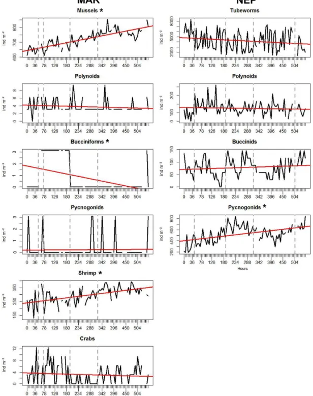
For MAR, 84 images in total were analysed from the TEMPO module; there were nine gaps in the imagery data series (Table 2). The most abundant visible species were Bathymodiolus azoricus mussels and Mirocaris fortunata shrimp, the numbers of the other taxa (crabs, polynoids, buc-ciniform gastropods, pycnogonids) being an order of mag-nitude smaller (hundreds vs. single occurrences; for densi-ties see Fig. 3.). An overall significant increase in mussel and shrimp densities was observed (R2=0.68, p < 0.001, and R2=0.32, p < 0.001, respectively; Fig. 3). Conversely, a significant negative trend was observed for the buccini-form gastropods (R2=0.19, p value < 0.001, Fig. 3). For the other taxa, no significant trends in densities were
ob-Figure 3. Temporal variations in faunal densities for MAR and NEP along with trend lines (in red) and MRT temporal groups (grey vertical dotted lines); x axis shows the sampling frequency every 6 h. Taxa with significant trends (p < 0.05) are marked with an asterisk.
served. Trends were removed prior to periodogram analyses, which revealed no significant rhythms in mussels, shrimp, crabs and bucciniform gastropods. Only for polynoid scale worms was a significant 18 h period observed, followed by significant periods at 90 h (5 × 18 h), 186 h (∼ 10 × 18 h) and 204 h (∼ 11 × 18 h) (Fig. A1 in the Appendix). Polynoids were mostly found on bare substratum though they ventured
on the mussel bed occasionally. In fact, 92 % of the tions were associated with bare substratum vs. 8 % observa-tions on the mussel bed. One large individual occupied the exact same area in 61 % of all images analysed (Fig. 2). Buc-ciniform gastropods were observed on the bare rock in the foreground further away from the fluid exit (Fig. 2). Pyc-nogonids (seven observations) and the occasional ophiuroid
(four observations) were observed mostly at the edge or on top of the mussel bed, further away from fluid flow. Segon-zacia mesatlantica crabs were mobile, some moving in the FOV, others appearing between the mussels. Their distribu-tion was rather heterogeneous but mostly associated with the mussel beds and shrimp presence. A Cataetyx laticeps fish was observed five times within the analysed time series – mostly in the background and not interacting actively with the other organisms. Its presence was only discernible based on the video footage (and not on the screen stills). The small patch of anemones observed below the probe featured 33 in-dividuals. No changes were documented over time for this taxon.
For NEP, 88 images were analysed from the TEMPO-mini module; there were five gaps in the imagery dataset (Table 2). Ridgeia piscesae tubeworms were the most abun-dant taxon assessed on imagery, adding up to several hun-dred visible (outside their tubes) individuals and with their tubes providing a secondary surface for the other organ-isms to occupy. Thus, several dozens of pycnogonids, up to a dozen of polynoids and a couple of buccinids were present on the tubeworm bush (for densities see Fig. 3). The strings of stacked limpets were not quantified. Only pycno-gonid densities showed a significant positive temporal trend (R2=0.23, p < 0.001, Fig. 3). For the other taxa, no signifi-cant trends were observed. Periodogram analyses carried out on the faunal densities with a 6 h period revealed a distinct 12 h frequency and harmonics for tubeworms, a single 12 h period (i.e. no harmonics) and 222 h (9.25 days) for poly-noids (Fig. A2). Buccinids also showed some significant fre-quencies at 174 h (7.25 days) and 204–228 h (∼ 8.8 days, Fig. A2), while none were observed for pycnogonids. Py-cnogonids showed distinct clustering behaviour and spatial segregation which were also observed for the other taxa (buc-cinids and polynoids), although to a lesser extent. Eight vis-its of a Pachycara sp. (Zoarcidae) were documented, during which the fish was present next to the tubeworm bush and sometimes hiding underneath it. No specific behaviour of the fish interfering with the fauna of the tubeworm bush was doc-umented.
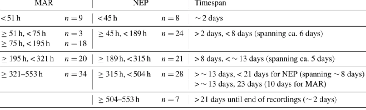
Different adjacent temporal groups were identified for MAR and NEP based on changes in faunal composition and densities over time through MRTs. Five temporal groups were delineated for NEP and MAR (Table 3) though they were partitioned differently over time. Most groups could be considered rather similar in time span for the two lo-cations. For the MAR, the highest variance was described by the split separating < 195 and ≥ 195 h. This coincided with an increase in shrimp and mussel densities and de-crease in gastropods and crab densities (Fig. 3), which were shown to be significantly indicative for different split groups post-195 h. Shrimp were found to be most indicative for the ≥ 321 h group (IndVal = 0.47, p < 0.05) and bucciniform gastropods for the ≥ 195 h to < 321 h group (IndVal = 0.78, p< 0.001). Bathymodiolus mussels were indicative for the
Figure 4. Percent microbial cover every 12 h for the imagery period analysed. The x axis contains periods; one period is equal to 12 h.
< 51 h group (IndVal = 0.45, p < 0.05) featuring the lowest densities for the studied time series. Contrastingly for the NEP, splits coincided with the chronology and tubeworm densities were significantly indicative for the < 45 h group (IndVal = 0.46, p < 0.001). Pycnogonids and buccinids were both indicative of ≥ 504 h (IndVal = 0.51, p < 0.001, and IndVal = 0.52, p < 0.001, respectively). The temporal split groups (Table 3) were delineated onto the faunal variation graphs (Fig. 3) and used to colour-code groups in the ordina-tions (see Sect. 3.1.3) in order to investigate how individual taxa and environmental conditions coincide with and influ-ence the temporal inconsistencies represented by the MRT groups.
Despite the large difference in percentage of the image covered by microbial mats between MAR (1.34–2.76 %) and NEP (25.11–37.02 %), both showed a decline during the pe-riod analysed (Fig. 4). The observed trends were significantly negative for both sites. For the MAR, this decline corre-sponded to a significant negative correlation between micro-bial cover and mussel densities (r = −0.67, p < 0.001) and shrimp densities (r = −0.53, p < 0.001). For the NEP, no sig-nificant correlations between microbial cover and other taxa were revealed.
3.1.2 Environmental data
Environmental data analysis presented in this section is a short-term analysis, spanning 23 days corresponding to the imagery duration.
Generally, higher temperatures were recorded at the MAR (Fig. 5). Mean temperatures at MAR were significantly higher than maxima recorded by probes T602 and T603 at NEP (Fig. 5, Table 4), coinciding with higher ambient seawater temperatures for the MAR (∼ 4◦C) than for NEP (∼ 2◦C). Even when rescaling to ambient temperature, min-imum temperatures measured on the MAR were still higher than those of the NEP. However, maximum and mean tem-peratures no longer stood out (but remained significantly
dif-Table 3. Temporal split groups for MAR and NEP based on MRT analysis. n is the number of images.
MAR NEP Timespan
< 51 h n =9 < 45 h n =8 ∼2 days
≥51 h, < 75 h n =3 ≥45 h, < 189 h n =24 > 2 days, < 8 days (spanning ca. 6 days) ≥75 h, < 195 h n =18
≥195 h, < 321 h n =20 ≥189 h, < 315 h n =21 > 8 days, < ∼ 13 days (spanning ca. 5 days)
≥321–553 h n =34 ≥315 h, < 504 h n =28 > ∼ 13 days, < 21 days for NEP (spanning ∼ 8 days)
> ∼ 13 days, 23 days (10 days for MAR)
≥504–553 h n =7 > 21 days until end of recordings (∼ 2 days)
ferent at p < 0.05) and were even lower than those measured by probes T602 and T603 in the NEP (Table 4). Standard de-viations and variance were maintained and were consistently higher at NEP but not significantly different.
The hourly temperature recordings showed noticeable cy-cles of higher and lower temperatures specifically in T602 and T603 (visible as red and blue colours in Fig. 6 respec-tively). When such (more or less) coherent bands of lower and higher values are observed in tidal pressure heat maps, it shows the cyclical nature of the tides. Hence, alongside the tidal rhythms revealed by the periodogram analyses, a tidal cyclicity was recognisable in the temperature recordings of the NEP. Patterns were less clear for the MAR temperature data. Information on pressure data from the same localities and correspondence to the temperature measurements was included as Appendix (Fig. A3).
In order to investigate how the temperature time series from the two oceans related to one another, cross correlations were carried out on the hourly temperature values (Fig. 7). Generally, positive autocorrelations were more pronounced, meaning that the two series were in phase. Maximum auto-correlation was reached at lag +5 h when comparing MAR to T602 with the MAR time series leading and a +5 to +6 h lag between MAR and T603. Most of the dominant cross correlations occurred between lags +4 and +7, with taper-ing occurrtaper-ing in both directions from that peak. This corre-sponded to the time difference of ∼ 6 h between MAR and NEP locations, calculated as follows: 24 × degrees (differ-ence in longitude)/360. Maximum negative autocorrelations were observed at lags −14 and +11 for NEP T602 and MAR and between lags +10 and +13 for NEP T603 and MAR. The difference between the maxima (and minima) closely corre-sponded to the tidal cycle (∼ 6 h).
There was a 6 h time difference in the Fe recordings car-ried out in the NEP being measured at 06:00 and 18:00 UTC and on the MAR at 12.00 and 00:00 UTC. Fe on the MAR was recorded twice a day (in four cycles) during the anal-ysed imagery period. Concentrations ranged from 0.41 to 1.62 µmol L−1with a mean of 0.81 ± 0.28 µmol L−1. A non-significant (p > 0.4) positive trend was observed but no
sig-nificant relationships between fauna, microbial cover and Fe were revealed. Fe measurements at NEP were limited to 7 days at a frequency of one measurement a day (Fig. 5). Consequently, its use as an explanatory variable for faunal variations was limited and no patterns were revealed. Values ranged from 2.07 to 2.99 µmol L−1, which were higher than those observed on the MAR but also showed less variation.
Turbidity measurements (NTU) were restricted to the MAR observatory and a non-significant positive trend was observed during imagery duration. A large peak was notice-able at ∼ 400 h (around 23 October 2011) though it was not reflected in any of the other environmental variables or com-munity dynamics (Fig. 5).
3.1.3 Fauna–environment interaction
Environmental variables incorporated in the ordination anal-yses did not distinguish significantly between faunal densi-ties or the temporal split groups found in the faunal compo-sition (Fig. 8). The first axis was most important for the MAR RDA (83.76 %), hence attributing a higher importance to the horizontal spreading, but was not significant (p > 0.05). This separation corresponded mostly with the separation of Miro-carisand Bathymodiolus. NTU seemed to have a distinct im-pact on separating the images from one temporal split group (from 51 to 195 h), though there was no clear signal in NTU values at that time. Overall, for the MAR, no distinct rela-tionship between a specific taxon and measured environmen-tal variables was revealed.
The first axis of the NEP RDA was significant at p < 0.005 and explained most of the variance (98.2 %) represented by the ordination plot (Fig. 8). This coincided with a separa-tion in the plot between Pycnogonida, Polynoidae and Buc-cinidae that pooled apart from the tubeworms. This lateral separation in taxa coincided with the strong correlation be-tween tubeworm densities (appearances) and the T602 and T603 temperature measurements. Only T603 was significant at p < 0.05. Temporal split groups were vertically aligned in the plot and tended to overlap, with tubeworms being more indicative for < 45 h group (as corroborated by the “multipatt indval” analysis). No clear influence from the environmental
Figure 5. Short-term environmental variables (23 days) averaged per hour during the imagery analysis period. Variables measured at both deployment sites are presented in the same graphic (temperature and Fe). Fe has a daily frequency for the MAR but a 12 h frequency for the NEP and recording times differ. NTU (nephelometric turbidity units) was only available for the MAR.
Table 4. Mean, maximum and minimum temperatures as measured by the probes and, for comparison purposes, rescaled to ambient seawater temperature (italic values). See Fig. 5 for significant differences in raw temperature values. Variance and standard deviations are presented as well. Bold values represent the highest values, which tend to change if rescaled to ambient seawater temperature or not.
Mean (◦C) Max (◦C) Min (◦C) Var SD
MAR 5.59 1.59 6.36 2.36 4.79 0.79 0.066 0.258
NEPT602 3.76 1.76 5.14 3.14 2.28 0.28 0.259 0.645
NEPT603 4.07 2.07 5.27 3.27 2.73 0.73 0.416 0.509
variables on the separation in temporal split groups could be revealed.
3.2 Long-term variability
Long-term variations in environmental conditions from both observatories spanning 9 months were investigated. As for the short-term analysis, the long-term time series analysed was limited by the shortest deployment period for which both observatories were up and running at the same time and was thus restricted by the TEMPO-mini observatory (NEP).
The continuous MAR temperature time series showed temperature variations between 4.48 and 10.91◦C, with a mean of 5.54 ± 0.71◦C (Fig. 9). A significant negative trend in temperature values was observed over the 9-month pe-riod; a trend already visible in the short-term analyses. The NEP temperature values recorded during this period by T602 and T603 were comprised between 2.23 and 5.43◦C, with a mean of 3.78 ± 0.54◦C. T602 showed a significant negative trend (p < 0.001) while T603 showed a significant positive
trend (p < 0.001) over the longer term. Trends were removed and periodogram analysis was carried out on the residuals for periods of 2 to n/2 (3168 h ∼ 4.5 months), 2 to 800 h (∼ 1 month) and 1-week periods (2 to 200 h). Regardless of the time span, diurnal and semi-diurnal periods and their har-monics were the main significant frequencies discerned. No clear or distinct significant hebdomadal (weekly) or infradian (multiple days) cycles were encountered. Therefore, in order to facilitate interpretation, only the periodograms with peri-ods of 2 to 200 h were presented (Fig. 10).
A significant period at 12 h was revealed for the MAR and NEP T602 probes but not for T603. For T603, a peak was present at T = 12 h but it was not significant; however, har-monics of that peak at 25, 37, 50, 74, 75 h (etc.) were signifi-cant (Fig. 10). A signifisignifi-cant 25 h period was thus observed for both NEP probes (T602 and T603). Recurrent harmonics of both semi-diurnal (12 h) and diurnal (25 h) frequencies were identifiable throughout the temperature time series, more so for NEP time series than for MAR, which agree well with
Figure 6. Hourly temperature values (◦C) for T602 and T603 probes from NEP and the MAR temperature probe. Red indicates higher temperatures while blue represents the lowest temperatures. Dates correspond to the duration of the imagery analyses (23 days).
Figure 7. Cross correlations of the hourly temperature values. ACF is the autocorrelation function on the y axis; one lag equals 1 h on the x axis. Comparisons are made between the MAR probe (T MAR) and T602 (NEP T602) on the left side and MAR (T MAR) and T603 (NEP T603) on the right. The horizontal dashed lines indicate the point of statistical significance at ACF = 0.8, with the lines above towards 1 and below towards −1 being significant.
the tidal cycle (12 h, 25 min and 24 h, 50 min) (Fig. 10). A distinct 6.25-day period (at 150 h) with a high amplitude was revealed for the T602 and T603 probes (Fig. 10). Such a peak was recognisable for the MAR as well, though it was not sig-nificant. A peak at 174 h (7.25 days) was significant for all three probes (MAR and NEP). The corresponding significant periods between MAR and NEP were thus 12, 37, 87, 112 and 174 h though some were less pronounced depending on the ocean.
For Fe, a negative, almost significant trend (p > 0.05) was observed for 6 months of data (30 September 2011– 29 March 2012) from the MAR featuring two Fe measure-ments a day (at 00:00 and 12:00 UTC) (Fig. 9). Minimum and maximum concentrations were 0.25 and 2.61 µmol L−1, re-spectively, with a mean of 0.98 ± 0.43 µmol L−1, which was
lower than the averaged concentrations of the other deploy-ment years (with 2.12 ± 2.66 µmol L−1averaged over 2006, 2010–2011, 2012–2013 and 2013–2014). Periodogram anal-yses revealed a peak at 108 h (4.5 days) and a more pro-nounced one at 180 h (7.5 days), but neither of these were significant. For the NEP, a time series of one Fe measure-ment a day (at 06:00 UTC), consisting out of four sampling cycles spanning > 4 months, was analysed (20 October 2011– 26 March 2012). The last 49 days (31 January–26 March 2012) were omitted due to artefacts visible in Fig. 9, which were due to the reagents running low. Periodogram analy-sis of these ∼ 3 months of data revealed no significant pe-riods either. Fe concentrations ranged from a minimum of 0.67 µmol L−1to a maximum of 5.45 µmol L−1, with mean values at 2.40 ± 1.03 µmol L−1. Mean values approached the
Figure 8. Redundancy analysis (RDA) ordinations featuring Hellinger-transformed faunal densities and environmental variables, both at a 6 h frequency. MARavg is the temperature time series from the MAR and NTU is turbidity. T602 and T603 were the NEP temperature probes. Temporal splits groups were colour-coded in the ordination plots.
Figure 9. Long-term environmental variable overview. Temperature time series at MAR and NEP represent hourly temperature data spanning 9 months. Fe was recorded over 6 months, twice a day at MAR and daily at NEP. Dotted vertical lines delineate the period for which the images have been analysed. Inset box in Fe graph for NEP shows variation occurring during the first 4 months in more detail.
maximum values measured by the MAR observatory, similar to what was observed in the short-term analyses.
Due to the unresolved issues with the optodes and the oxy-gen concentrations measured (see Sect. 2.2), only the differ-ences in overall concentration were used to describe the dif-ferences between the two sites. For the MAR, measurements ranged from 170.54 to 251.66 µmol L−1 with a mean of 230.62 ± 16.98 µmol L−1. The NEP featured distinctly lower concentrations, ranging from 23.67 to 77.26 µmol L−1with
a mean of 63.42 ± 7.15 µmol L−1. Here there also seemed to be more variability at the NEP than at the MAR.
Turbidity was only measured at the MAR observatory and showed several large peaks further along in the long-term time series (e.g. during end February 2012 and May to June 2012) (Fig. 9), but none of these observations translated themselves in the other environmental variables. There was a significant positive trend for NTU over 9 months (p < 0.001) but no significant periods were revealed by the periodogram analyses.
Figure 10. Periodogram analyses of ∼ 9 months of hourly tempera-ture measurements for MAR and NEP (T602 and T603) represented as a 1-week period (equalling 200 h). One period is equal to 1 h. Black squares indicate periods significant at the 5 % level.
4 Discussion
4.1 Comparison in faunal composition
The two observatories each filmed one single assemblage over time in a limited FOV, whereas hydrothermal edifices are characteristically inhabited by mosaics of different fau-nal assemblages, spatially distributed according to local en-vironmental conditions and microhabitats (e.g. Sarrazin et al., 1997, 2015; Cuvelier et al., 2009, 2011a), patterns that are enhanced by high local variability in environmental vari-ables at centimetre scales and steep physico-chemical gra-dients (Sarrazin et al., 1999; Le Bris et al., 2006). The two different study sites also feature different spreading rates, which may influence community dynamics at vents by cre-ating less habitat stability in higher spreading rate settings (Tunnicliffe and Juniper, 1990; Shank et al., 1998). While relative stability in faunal composition has been observed on a number of edifices, even reaching decadal-scale stability at some (e.g. Eiffel Tower), smaller-scale variations, both in space and time, do occur (Cuvelier et al., 2011b). Hence, the variations in faunal densities observed during this study may not apply to the hydrothermal edifice as a whole; the presence of rhythms in the organisms and in temperature, although ob-served on a smaller surface, is likely to apply for the entire hydrothermal structure.
Vent fauna hosted by the two study sites are quite differ-ent. While there are similarities at higher taxonomic levels, e.g. classes and families, there is only one correspondence on genus level (Sericosura sp., Pycnogonida) and none on species level between both sites. A higher number of visible taxa were identified on MAR images when compared to NEP (8 vs. 6, respectively, not taking into account microbial cover or visiting fish species). This observation does not imply that the MAR is more diverse than the NEP since imagery only gives a partial overview of the actual diversity (Cuvelier et al., 2012). When comparing samples, an overall higher di-versity was observed in the Pacific than in the Atlantic hy-drothermal vent ecosystems, with species richness being pos-itively correlated with spreading rate, associated distance be-tween vent fields and longevity of vents (Juniper and Tunni-cliffe, 1997; Van Dover and Doerries, 2005). Nevertheless, such observations remain subject to how well a certain lo-cality is studied and if all faunal size fractions (meiofauna to megafauna) are included in assessing diversity (e.g. Sarrazin et al., 2015). Diversity estimates represent one of the main limitations of imagery analysis, which is limited to quanti-fying and correctly identiquanti-fying (assessing) mega- and macro-fauna (∼ mm). In the subsequent sections temporal variations and behaviour (rhythms) of the separate taxa and their impli-cations for possible microhabitat and niche occupation will be discussed.
4.1.1 Engineering species
Bathymodiolus azoricusmussels visually dominate the shal-low water (< 2300 m) vents along the MAR and appear to be a climax community, being present for a few decades on the same edifices within the Lucky Strike vent field (Cuvelier et al., 2011b). They form dense faunal assemblages in relatively low-temperature microhabitats (De Busserolles et al., 2009; Cuvelier et al., 2011a). A spatial segregation in mussel sizes is observed with a decrease in size with increasing distance from hydrothermal input and corresponding thermal gradi-ent showing diet changes with mussel size categories (Hus-son et al., 2017). Contrastingly to what has been described by Sarrazin et al. (2014), no significant interactions between mussels and other organisms were observed based on the 6 h frequency analysed here.
Tubeworms of the species Ridgeia piscesae are the main visible constituents of the filmed assemblage at NEP and a secondary surface for the associated fauna assessed here. Their appearance rate showed a strong relationship with the temperature recorded by probes T602 and T603 (Cuvelier et al., 2014, and this study) in contrast to the other taxa. Emer-gence/retraction movements of siboglinid tubeworms were proposed to be a thermoregulatory behaviour or suggested to be governed by oxygen or sulfide requirements (Tunni-cliffe et al., 1990, Chevaldonné et al., 1991) or tolerance to toxic compounds (sulfides, metals, etc.). Changing hy-drothermal inputs (high sulfide concentrations/high
temper-ature) and oxygen concentrations could thus regulate tube-worm appearances, reflecting the tidal patterns of these envi-ronmental variables. Whilst interactions between tubeworms and other taxa were not significantly quantifiable on the cur-rent 6 h frequency of image analyses, they have been ob-served and described for the hourly frequency (Cuvelier et al., 2014).
4.1.2 Shared taxonomic groups
Many of the free-living polynoid species are known as active predators (Desbruyères et al., 2006) moving rather swiftly across the FOV looking for prey and were even observed at-tacking extended tubeworm plumes at NEP (Cuvelier et al., 2014). Free-living MAR scale worms were preponderantly associated with bare substratum, while those quantified for NEP were only those observed on top or within the tube-worm bush. They were also visible on the bare substratum surrounding the tubeworm bush but this area was not taken into account during this study. While there was a difference in substratum association between polynoids as observed by the two observatories, all individuals seemed to be rather ter-ritorial (see Cuvelier at al., 2014). On the MAR, one individ-ual appeared to repeatedly return to one single area within the FOV after excursions. Such behaviour might be indicative of topographic memory and homing behaviour. The Atlantic commensal polynoid Branchiplynoe seepensis can occasion-ally be observed outside of the mussel shells (Sarrazin et al., 2014), wherein it normally resides, but not on the image se-quence analysed here.
Buccinid (NEP) and bucciniform (MAR) gastropods ap-peared more related to less active environments. Both species are considered predators or scavengers (Desbruyères et al., 2006; Martell et al., 2002). Within the MAR setting, snails (Phymorhynchus sp.) were present in very low abundances (one or two individuals at most) and were positioned on bare rock with no fluid flow. In the NEP setting, whelks (Buc-cinum thermophilum) were generally more abundant in ar-eas inhabited by vent animals. No correlation with emerging fluid temperatures was observed nor was a substratum pref-erence revealed (Martell et al., 2002). Abundances observed within the FOV tended to vary from one to six individuals, while they were shown to congregate in groups of five or more individuals at MEF (Martell et al., 2002).
Sea spiders (Pycnogonida) showed a very distinct spa-tial distribution at NEP featuring a localised clustering be-haviour (see heat maps published in Cuvelier et al., 2014), whilst their presence on the MAR was occasional. MAR py-cnogonid individuals were only observed visiting the edge of the mussel bed which was further away from the fluid exit. A large difference in pycnogonid densities (ind m−2) was observed between the two sites as well, with a ratio of 1/250 MAR vs. NEP. Increased activity and aggregations of more than five individuals (and increased intra-species con-tact) at NEP were linked to conditions of high-temperature–
low-oxygen saturation (Lelièvre et al., 2017). Interestingly, these organisms all belong to the same genus, namely Seri-cosura. The species known for the Lucky Strike vent field (MAR) is Sericosura heteroscela, while there are multiple species (within the same genus) for the Main Endeavour Field (NEP), among which is Sericosura verenae. All Seri-cosuraspecies from the Ammotheidae family known so far appear to be mostly obligate inhabitants of hydrothermal vents or other chemosynthetic environments (Bamber, 2009). While being an abundant taxon with a localised clustering behaviour at the NEP site, it is scarce and vagrant at the MAR. Their microhabitat and niche occupation at the studied sites is likely to differ, causing the discrepancies observed.
The generic term microbial cover is used to refer to the microbial mats colonising various surfaces in the vent en-vironment without assuming similar microbial composition. While no significant relationships were revealed between mi-crobial cover and fauna for NEP in the current study, a signif-icant negative correlation was observed for this site between pycnogonids and microbial cover based on the same imagery analysed with a higher frequency (4 instead of 12 h), which was attributed to pycnogonid grazing (Cuvelier et al., 2014). For MAR, significant negative correlations existed between microbial coverage and mussels and microbial coverage and shrimp. For the mussels, this could be due to scattering and repositioning of individual mussels: as mussel reposition on top of the microbial mats, they decrease the visible and as-sessable microbial coverage. The negative relationship be-tween shrimp and microbial cover could be caused by the shrimp grazing on microorganisms (Gebruk et al., 2000; Co-laço et al., 2002; Matabos et al., 2015).
4.1.3 Regional taxa MAR
The hydrothermal alvinocaridid shrimp observed by the MAR observatory mostly belong to the Mirocaris fortunata species. On the images analysed, they were most abundant in the main axe of flux. Matabos et al. (2015) quantified this to about 60 % of the shrimp abundances (to 69 cm of an emis-sion), confirming previous distributional patterns of shrimp being indicative of fluid exits and characteristic for warmer microhabitats (Cuvelier et al., 2009, 2011a; Sarrazin et al., 2015). Their thermal resistance and tolerance corroborates this pattern (Shillito et al., 2006). Because their distribution is linked to the presence of fluid exits and flow, a significant positive correlation between shrimp and temperature would be expected. To date, however, such a relationship could not be designated in this study or in previous studies based on data from the deep-sea observatories (Sarrazin et al., 2014; Matabos et al., 2015), though Sarrazin et al. (2014) did show a significant positive correlation between Mirocaris fortu-nataabundances and vent fluid flux.
Segonzacia mesatlantica crabs (Bythograeidae, De-capoda) were mostly associated with the mussel beds and anhydrites, as were the shrimp (Matabos et al., 2015). Some interactions between crabs and shrimp were observed, mostly resulting in shrimp fleeing. Possible significance of these in-teractions (mostly territorial in nature) was described in more detail by Matabos et al. (2015).
The fish Cataetyx laticeps (Bythitidae, Osteichthyes) was frequently observed at the base of the Eiffel Tower edifice within the Lucky Strike vent field (Cuvelier et al., 2009). No feeding on the benthic hydrothermal fauna was observed dur-ing the 6 h frequency image analyses.
NEP
Contrastingly to the 1 h frequency observations (Cuvelier et al., 2014), no spider crabs (Majidae) were observed visiting the filmed assemblage on a 6 h frequency imagery analyses. Whilst this majid spider crab is known as a major predator in hydrothermal vents, no such actions were recorded by our observatory module.
Similarly to Cataetyx fish on the MAR, no visible activi-ties of feeding or predation of Pachycara sp. eelpouts (Zoar-cidae) were observed on the NEP. Cuvelier et al. (2014) pro-posed that the eelpouts (and fish in general) may be more sen-sitive to the effects of lights but this hypothesis, based on be-havioural observations, could not be confirmed in the present study due to the low-resolution observation frequency. 4.2 Short-term variations and rhythms in fauna and
environment
When looking at the engineering taxa for each ocean, a clear diurnal rhythm was observed in visible (i.e. out of their tubes) tubeworms (NEP), while there was a lack of temporal rhythms in mussel densities (MAR). However, taking into ac-count the characteristics of both chemosynthetic taxa, ac-counts of mussels with open valves and extended siphons instead of densities should be used for comparison to tubeworms out-side their tube. This difference in assessment could account for the lack of temporal periodicities at the MAR, where mussel valve openings or visible siphons were impossible to quantify due to the larger distance between the observatory and the filmed assemblage. Different causes might trigger a mussel to open his valve or a tubeworm to come out of its tube and these can be either attributed to an external trigger (e.g. retraction or closure after possible predation actions; for tubeworms, see Cuvelier et al., 2014; for mussels, see Sar-razin et al., 2014) or to their physiology (need for nutrients or saturation). No significant links have yet been established between fluid flow and open mussel valves (Sarrazin et al., 2014) but some indications of tidal rhythmicity were visible (Matabos et al., unpublished data). No consistent statistically significant link between fluid flow and tubeworm appearance has been revealed to date either (Cuvelier et al., 2014),
al-though a steady significant semi-diurnal tidal rhythm over time was observed. The niche occupation and role within the ecological succession over time of mussels and tubeworms are very different for the two oceans. In Pacific monitor-ing studies, tubeworms are out-competed by mytilid mussels when hydrothermal flux start to wane (Hessler et al., 1985; Shank et al., 1998; Lutz et al., 2008; Nees et al., 2008), while the latter appear to represent a climax community in the more stable Atlantic < 2300 m (Cuvelier et al., 2011b). Neverthe-less, a 23-day period appears too short to allow observation of succession patterns.
Next to the engineering species, only a few other taxa showed significant periodicities in densities over time, namely polynoids for MAR and NEP and buccinids for NEP. The lack of significant periodicities in MAR shrimp was cor-roborated by a long-term study by Matabos et al. (2015). Both polynoids and buccinids displayed multiple-day peri-odicities instead of tidal cycles, which could be mostly re-duced to harmonics of tidal cycles that become more visible further along in the time series as they become more pro-nounced over time. For both taxa, the multiple-day period-icities approached those visible in Fe, i.e. 4.5 and 7.5 days (though non-significant), and besides an apparent preference for lower temperatures there were no significant links with temperature (as corroborated by Lelièvre et al. (2017) for the polynoids). Additional high-resolution investigations will be necessary to corroborate or validate these observations. Overall, the reasons for the lack of periodicities in fauna can be twofold: either the taxon in question is unevenly repre-sented in low abundances and therefore too heterogeneous (rendering any statistical test difficult which was the case for MAR crabs and pycnogonids) or the recording/analysing fre-quency does not allow discerning of significant periods. The shortest period to be resolved is twice the interval between the observations of a time series. Hence, caution is needed when interpreting patterns as the recording and analysing fre-quency influences observations. A previous higher-resolution study (hourly frequencies) already showed that, depending on the frequencies investigated, the type of relationships (significance, positive or negative) between the taxa might change (Cuvelier et al., 2014).
While certain environmental variables might explain a large amount of variation occurring in a single taxon (e.g. NEP tubeworm appearances and temperature from probes T602 and T603), a wider variety of environmental variables measured at multiple sampling points across the FOV in a resolution similar to or higher than the imagery analyses fre-quency should be considered in order to explain and compre-hend the whole of community dynamics. This was also illus-trated with the temporal split groups identified in community composition constrained by time, where the predictive power of the split groups was rather low and groupings could not be corroborated with changes in the environmental variables. Split groups were quite similar for the larger groups (those with higher n) with those at the MAR occurring 6 h later
than those at the NEP. A slower pace in significant detectable changes in overall faunal composition in the Atlantic vs. the Northeast Pacific could be explanatory. For instance, differ-ence in spreading rate was shown to be directly proportional to different rates of change in community dynamics between slow-spreading MAR and faster-spreading NEP (Cuvelier et al., 2011b).
4.3 Long-term environmental variations and rhythms In hydrothermal vents, temperature is a proxy of sulfide and Fe concentrations and most importantly of the hydrothermal vent input. Highest minimum temperatures were recorded at the MAR where the probe was positioned closer to a visi-ble fluid exit, whereas NEP temperatures were more variavisi-ble and displayed broadest ranges. It is important to bear in mind that ambient seawater temperature at 1700 m on the MAR is higher than that at 2200 m depth in the NEP (4◦C vs. 2◦C respectively). When taking this into account and rescaling the temperature values, mean and maximum temperatures were highest at NEP. Highest positive and significant auto-correlation values indicated a ∼ 5–6 h lag between MAR and NEP, with MAR leading. Interestingly, the hour difference between the two sites corresponds to ∼ 6 h as well. The ge-ographical distance separating the two localities thus allows us to quantify not only the time difference between two sites but also the delay in the tidal rhythms observed between the two.
Tidal rhythms were discernible in both NEP and MAR temperature series. Potential mechanisms causing tide-related variability in hydrothermal fluids included the mod-ulation of seafloor and hydrostatic pressure fields by ocean tides, modulation of horizontal bottom currents by tides and solid earth tide deformations (Schultz and Elderfield, 1997; Davis and Becker, 1999). For NEP, diurnal periods at ∼25 h were discerned for both temperature probes (T602 and T603). Significant semi-diurnal periods were also found in T602, though for T603 they could only be identified based on their harmonics. The MAR temperature time series also had a distinguishable semi-diurnal component. Tidal rhythms ob-served in the temperature time series for NEP and MAR were concordant with observed tidal signals for the respective re-gions. For instance, in the NEP, measured tides in the Barkley Canyon, another instrumented node from ONC closer to shore, were mixed semi-diurnal/diurnal at 870 m depth (Ju-niper et al., 2013). In the same canyon, periods of enhanced bottom currents associated with diurnal shelf waves, inter-nal semi-diurinter-nal tides and wind-generated near-inertial mo-tions were shown to modulate methane seepage (Thomsen et al., 2012). While temperature variability in hydrothermal vents at Cleft Segment on the Juan de Fuca Ridge was shown to greatly diminish when current directions did not shift in direction with the tides, it was suggested that, through the modulation of horizontal bottom currents, the modulation of temperature by tides was only indirect (Tivey et al., 2002).
These horizontal bottom currents showed 12.4 h tidal period-icity which was also found in the temperature time series of the aforementioned article as well as in our NEP tempera-ture time series. Consistent with the main orientation of the ridge and the topography of Grotto, temperature and oxy-gen saturation at the NEP deployment site were shown to be strongly and significantly influenced by the northern and southern horizontal bottom tidal currents (along the valley axis) (Lelièvre et al., 2017). Patterns in temperature varia-tion of the MAR time series corresponded to the tidal signal observed in the Lucky Strike vent field at 25 h and to the semi-diurnal tidal oscillation at 12:30 h (Khripounoff et al., 2000, 2008).
Between oceans, differences were observed in tidal rhythms of high (> 200◦C) and low (< 10◦C) temperature records. For the NEP, the tidal influence appeared to wane in high-temperature records, making tidal signals less clear or even non-existent (Tivey et al., 2002; Hautala et al., 2012). While for the MAR the semi-diurnal variability in the high-temperature records was shown to be more significant and to be more coherent with pressure than those observed in low-temperature records (Barreyre et al., 2014). Unfortunately, we cannot corroborate this with the current study as only low-temperature time series were recorded by both ecolog-ical observatories. Even though we revealed some similari-ties in the rhythms of MAR and NEP low-temperature series collected for the same period, there were indications that lo-cal hydrography and associated bottom currents play a major role on the temporal variability of diffuse outflow and vent discharges (Barreyre et al., 2014, Lee et al., 2015). Clear peaks in temperature variables were noticeable at ∼ 6–7 days in MAR and NEP. We do not know what caused this period to be significant. In comparison, at Cleft Segment more south-wards on the Juan de Fuca Ridge (NEP), Tivey et al. (2002) found 4–5-day broadband peaks in temperature from diffuse flow as well as high-temperature vents which were thought to be storm-induced from the sea surface.
Fe is commonly used as a proxy for vent fluid composi-tion. Higher Fe concentrations would thus be expected where temperatures were higher, in this case at MAR (vs. NEP). However, the opposite was observed here. The Fe concen-trations reported here for the MAR were lower than the Fe concentrations from other deployment years at the same site (Laës-Huon et al., unpublished data). The 2011 concentra-tions recorded at the MAR were close to the detection limit of the CHEMINI instrument (0.3 µmol L−1). Additionally, the MAR system was not calibrated in situ, contrastingly to the NEP, which could have generated a lower accuracy in the calculated concentrations, though question remains if such large discrepancies can be explained by this feature alone. The location of the sample inlet and the high spatial varia-tion occurring in hydrothermal vents might contribute to the patterns observed. The values observed at NEP were of the same order of magnitude as those reported for the Flow site also on the Juan de Fuca Ridge (i.e. 0 to 25 µmol L−1;
Tunni-cliffe et al., 1997). No significant periods (based on 12 or 24 h recording frequency) were found at the sites for the duration of the deployment, although some indications of 4.5- and 7.5-day periodicities could be observed at the MAR and 3.8-day cycles for Fe concentrations were detected in the same sampling area for 2012–2013 (Laës-Huon et al., 2017). For the NEP, 4-day oscillations in currents near seamounts along the crest of the Juan de Fuca Ridge were observed (Cannon and Thomson, 1996), but these were not visible in the Fe time series at NEP, although 4.5-day periodicities were visi-ble in buccinids and polynoids (Cuvelier et al., 2014). Hence, there were some indications of multiple-day periodicities, but these findings need to be corroborated, preferably by using a higher sampling frequency.
Turbidity (NTU) levels observed showed several large peaks over time. Particle flux at Lucky Strike combines both large and small diameter particles which have differ-ent settling velocity (Khripounoff et al., 2000). Kripounoff et al. (2008) showed an increased particle flux in April that reached a maximum at the end of May (2002). These do not correspond to the peaks observed here (in this study peaks were most pronounced at the end of October, February to March and May to July) but turbidity peak occurrences tend to differ between years and seasons. Due to seasonal peaks, longer time series will be needed to reveal recurrent patterns. Generally, multiple-day periodicities were harder to re-veal as many of them can be reduced to harmonics of the tidal cycles. In this perspective, the long(er)-term environ-mental variable analyses were considered more robust due to increased number of data points. Nevertheless, there is not much we can currently say on multiple-day or hebdomadal cycles observed in the time series presented here.
4.4 Limitations
Overall in hydrothermal vents, it remains hard to establish relationships among the environmental variables measured in situ. Ratios of temperature to chemical concentrations are not constant and can vary between sites (Le Bris et al., 2006; Luther et al., 2012). There is also the issue of high variance (and noise) in environmental variable time series as well as that of a possible delay in appearance of certain peaks, which makes it difficult to unravel patterns. Such a delay between environmental variable recordings might exclude the abil-ity of unravelling/exposing correlations. The example for Fe and temperature recordings, where a delay of 1 to 5 min cluded a direct correlation for each sample point, was pre-sented by Laës-Huon et al. (2016).
Caution is needed when programming the recording fre-quencies of imagery and environmental variables. Despite being mainly restricted by battery life (wireless observato-ries), light usage (wired observatories) or quantity of reagents (both), a 6 h analysing frequency might not be the most rep-resentative to assess faunal variations and links with the envi-ronment. Indicative of this are the differences observed when
analysing different frequencies as briefly touched upon in Cuvelier et al. (2014) and comparing them with those pre-sented here. It still proves difficult in hydrothermal vents to link faunal variations with single-point environmental vari-ables measured in situ. This can be attributed to the high spatial and temporal variation of the environmental gradients compared to the larger FOV assessed and to the recording frequencies or complexity of in situ measurements with cor-rections to be applied and possible delays. Temperature still seems the best proxy for faunal variations, but not all fau-nal presences/absences, abundances or the entirety of com-munity dynamics can be explained solely by temperature. Biotic interactions are at play as well. While these can be observed thanks to the remote observatory set-up, long-term high-resolution data need to be assessed (Matabos et al., 2015).
The influence of the lights on the fauna was hard to discern during this study, though supposedly fish presence would be more impacted when compared to invertebrate fauna (Aguzzi et al., 2010; Cuvelier et al., 2014).
Deployment of probes has also proven to be a predica-ment. While more accessible sites tend to be preferred and selected, deployment setting, accessibility, underwater con-ditions (e.g. currents), ROV (remotely operated vehicle) ma-noeuvrability and piloting skills also influence the final ob-servatory set-up.
5 Conclusions
Influence of the tides is visible in both settings, most clearly in temperature variables and in tubeworms appearances. The geographical distance separating the two localities is shown to quantify not only the time difference between two sites but also the delay in the tidal rhythms observed in temperature values (which is at a ∼ 6 h lag) between the MAR and NEP. Temporal split groups in community composition are rather similar between both settings, though the 6 h delay is visible as well. Shared taxa comprised one genus (Sericosura), one family (Polynoidae) and one class (a buccinid and a buccini-form Gastropoda) and, based on their relative abundance and behaviour, they seem to occupy different niches in the differ-ent hydrothermal vdiffer-ents. Nevertheless, it remains complicated to unravel links with the environment and to discern which environmental variable is the most influential or explanatory. To date, temperature remains the most explanatory, though it cannot explain the entirety of community dynamics. This is likely due to the high spatial variation at hydrothermal vents and the single-point measurements done by the environmen-tal probes. A persistent need remains for more complemen-tary and representative data, measured at frequencies similar or higher than the imagery recordings and at multiple points in the FOV. Recording frequencies are crucial: a 6 h record-ing frequency might not be good enough to represent the in situ reality. Also the implementations of instruments that do
not imply complex tools but allow the assessment of addi-tional environmental variables (e.g. current metres) could be a way forward. Automated and semi-automated tools should be developed for specific taxa and settings to assist in assess-ing faunal abundances in images.
Data availability. Data from TEMPO EMSO-Azores
obser-vatory 2011 deployment (MAR) are publicly available at https://doi.org/10.12770/bac2a0e5-58d1-40c9-b0aa-3a106e7ca7eb (Cannat et al., 2015).
Data from Tempo-mini (ONC Canada) (NEP) are avail-able through Ocean Networks Canada website http://www. oceannetworks.ca/ and their data portal http://dmas.uvic.ca.
Appendix A
Figure A1. MAR faunal periodogram on polynoid densities with a 6 h frequency (1 period on x axis is equal to 6 h) of 23 days; all other taxa had no significant periodicities and were thus not shown. Black squares indicate periods significant at the 5% level.
Figure A2. NEP faunal periodograms of 23 days featuring signifi-cant periodicities. Taxa presented are tubeworm, polynoid and buc-cinid densities with a 6 h frequency for the MAR (1 period on x axis is equal to 6 h); pycnogonids showed no significant periodici-ties and were not shown. Black squares indicate periods significant at the 5 % level.
Figure A3. Comparison of cyclicity in pressure data and temperature for (a) MAR and (b) NEP. Red shows higher values while blue indicates the lowest values. Pressure data for MAR originate from 2007 to 2008 and were recorded at SeaMoN West of the EMSO-Azores observatory and represents a random 28 day (lunar) period (data courtesy of Valerie Ballu). Pressure data for NEP were downloaded from ONC Portal from the BPR (NRCan Bottom Pressure Recorder deployed at MEF/Endeavour) (Ocean Networks Canada Data Archive, http: //www.oceannetworks.ca; total pressure data from 1 to 29 October 2014, University of Victoria, Canada, downloaded on 16 June 2015). A random selection of 28 days in October 2014 is presented here (no earlier data were available).