Predicting Market Impact Costs Using Nonparametric Machine Learning Models.

(1)

Predicting Market Impact Costs Using

Nonparametric Machine Learning Models

Saerom Park1¤a_{, Jaewook Lee}1¤a_{, Youngdoo Son}2,3¤b

*

1Department of Industrial Engineering, Seoul National University, Seoul, South Korea,2Research Institute of Engineering and Entrepreneurship, Seoul National University, Seoul, South Korea,3Department of Industrial and Systems Engineering, Rutgers University, Piscataway, New Jersey, United States of America ¤a Current address: 39-311, Seoul National University, 1 Gwanak-ro, Gwanak-gu, Seoul 151-742, South Korea

¤b Current address: A203, Engineering Building A-wing, Rutgers University, Piscataway, New Jersey 08854, United States of America

*hand02@snu.ac.kr

Abstract

Market impact cost is the most significant portion of implicit transaction costs that can reduce the overall transaction cost, although it cannot be measured directly. In this paper, we employed the state-of-the-art nonparametric machine learning models: neural networks, Bayesian neural network, Gaussian process, and support vector regression, to predict mar-ket impact cost accurately and to provide the predictive model that is versatile in the number of variables. We collected a large amount of real single transaction data of US stock market from Bloomberg Terminal and generated three independent input variables. As a result, most nonparametric machine learning models outperformed a-state-of-the-art benchmark parametric model such as I-star model in four error measures. Although these models encounter certain difficulties in separating the permanent and temporary cost directly, non-parametric machine learning models can be good alternatives in reducing transaction costs by considerably improving in prediction performance.

Introduction

Transaction cost is one of the important factors that affect the investment performance and is usually classified into two major categories: explicit costs and implicit costs. Explicit costs, also called direct costs, are transaction costs that can be explicitly stated and measured. These costs include commissions, transaction fees, and taxes. Implicit costs, or indirect costs, are costs that cannot be measured directly but can be improvable by an appropriate trading strategy. They include bid-ask spreads, time risk costs, and market impact costs.

Market impact cost, one of the implicit transaction costs, is the cost caused by the difference between the price before the transaction and the actual price that the transaction is executed actu-ally. During the last decade, many studies have been focused on analyzing market impact costs by not only the academic researchers but also the practitioners because it is one of the main reducible parts of the transaction cost. [1] and [2] fitted the impacts of single transactions to a concave

OPEN ACCESS

Citation:Park S, Lee J, Son Y (2016) Predicting Market Impact Costs Using Nonparametric Machine Learning Models. PLoS ONE 11(2): e0150243. doi:10.1371/journal.pone.0150243

Editor:Yingfeng Zhang, Northwestern Polytechnical

University, CHINA

Received:October 28, 2015

Accepted:February 2, 2016

Published:February 29, 2016

Creative Commons Attribution License, which permits unrestricted use, distribution, and reproduction in any medium, provided the original author and source are credited.

Data Availability Statement:The authors of this study obtained all relevant data from the Bloomberg terminal which can be accessed by subscribing to the Bloomberg Professional service (http://www. bloomberg.com/professional/,software@bloomberg. net).

Funding:This work was supported by the National

(2)

power-law function of the volume of the transaction. [3] used a logarithm function of the transac-tion volume to estimate market impact costs. [4] exploited the hyperbolic tangent function for the same task. [5] and [6] used a stochastic process of the asset price which includes a function of the transaction size to explain market impacts. [7] estimated impact cost by using a linear regres-sion with quantized transaction sizes. [8] analyzed the market impacts of the large institutional orders in the US equity market and found that the permanent impact function has a concave form with respect to the transaction size, in contrast to the previous results [5,9] in which the per-manent impact function had a linear form. The I-star model, a state-of-the-art parametric model, described in [10] and [11] is a log-linear regression model that uses three inputs, transaction size, volatility, and underlying trading rate. These inputs affected the estimated market impact costs independently. [12] and [13] used more than 40 independent variables to fit the market impact cost to simple linear regression function. However, those existing parametric approaches showed the limitation in estimation and prediction performance because they assumed the fixed paramet-ric or simple linear regression form of the market impact model. In addition, most of them cannot employ the variables that are not originally included in the model thus a new model is always required to predict the market impact with the different set of variables.

Recently, nonparametric machine learning models have been successfully applied to diverse financial applications because of their abilities in fitting and predicting performances for com-plex data sets. They include the stock price prediction [14–17] and its derivative markets [18–

20], credit and its derivative markets [21–23], fixed-income markets [24,25], and foreign exchange markets [26,27].

In this paper, we introduce nonparametric machine learning approaches to estimate and predict market impact costs more accurately than the existing parametric approaches. To our knowledge, this is the first approach that applies several nonparametric learning models to ana-lyze the market impact cost. The proposed nonparametric approach has two main advantages. First, the nonparametric approaches usually fit the data better than does the parametric case. Second, the nonparametric approaches are versatile in the number of input variables so the general procedure does not change, whereas the number or kinds of input variables change while the parametric approaches require the new parametric models in those cases. By simula-tion, we analyzed the market impact costs of transactions of small-cap, mid-cap, and large-cap stocks in US equity market both altogether and separately by selecting the same types of input variables with I-star model [10,11] and compared the results.

The remainder of the paper is organized as follows. In the next section, we briefly explain the I-star model which is used as a parametric benchmark with three input variables. Then, we describe how to use nonparametric regression models to construct market impact cost func-tions. Data description and experimental procedures with the experimental results are pre-sented in the following sections. Finally, we provide the summarized results, limitations, and some directions for the future work in the discussion section.

Review of I-star model

In this section, we first briefly review I-star model [10,11] which is a state-of-the-art bench-mark parametric model. I-star model, which uses three input variables to describe the bench-market impact cost, is composed of two separated equations calculatingI, a theoretical instantaneous cost, andMI, the market impact cost appeared in the real market, respectively. The equations calculate them are given as follows:

I _¼_a

1Size

a2_Vola3 _ð₁_Þ

MI ¼b1IPOVa4þ ð1 b1ÞI ð2Þ

study design, data collection and analysis, decision to publish, or preparation of the manuscript.

Competing Interests:The authors have declared

(3)

whereSize,Vol, andPOVare input variables anda1,a2,a3,a4, andb1are parameters to be determined.

The first input variable of Eqs (1) and (2) isSize, the normalized order size. Based on [11], this variable is represented asSize=Q/ADV, whereQis the imbalance, the absolute value of difference between buy order and sell order, andADVis 30-day average daily volume. Thus

Sizeimplies the magnitude of pressure from this order relative to the average daily volume. The second input variable,Vol, is the volatility of the equity return and 30-day averaged volatil-ity was used in [11]. The last input variable,POV, is an acronym forpercentage of volumeand it reflects the market liquidity condition. [11] simply expressedPOV=Q/(Q+V) whereVis the expected volume traded for the period of time that the imbalance orderQis executed. If the market is liquid or the imbalance trade orderQis executed slowly,Vbecomes large and thus

POVbecomes small. SmallPOVresults in smallMIvalue so the market impact cost will be small when the market is liquid.

The market impact cost inEq (2)comprises two components, temporary impact cost and permanent impact cost which are the first and the last term in the right hand side ofEq (2)

respectively. Considering thatSizeandVolare used to calculate the value ofI, they affect both the temporary and permanent part of the market impact. However, the other input variable

POVonly appears in the temporary impact part. This result implies that the smallerPOV

incurs the smaller market impact cost when the other input variables are invariant. However, this effect is temporarily and the permanent impact on the market is independent of the market liquidity condition.

Several parameters should be estimated. These parameters can be determined with data sets, including input variable values and market impact costs observed in the market, by general parameter estimation techniques such as nonlinear optimization and grid search.

Nonparametric regression models

In this research, four state-of-the-art nonparametric machine learning models are used to esti-mate market impacts. As a preliminary, brief explanations of them are given as follows.

Neural networks

Neural networks [28] are nonparametric nonlinear regression models which can be fit to highly nonlinear data distribution. Mimicking a human brain, a neural network model consists of lay-ers that contains several nodes, conducting the same role with neurons in the human brain. Each node in the layer takes output values of all nodes in the previous layer as input values, cal-culates the output value, and provides the output value to all nodes in the next layer as one of their input values. The most common way of output value calculation in the node is as follows:

y¼fðX

i

wigðxiÞÞ ð3Þ

whereyis the output value of the node,xirepresents input value from nodeiin the previous layer,g() is an input transform function,wirepresents weights for input values, andf() is an activation function that makes the regression model nonlinear. The sigmoid functions, such as logistic function, probit function, and hyperbolic tangent function, and a liner rectiﬁed func-tion, for example,f(x) = max{0,x}, are usual selections for the activation function.

Finding optimal weights,wi, inEq (3)is the main task of constructing the neural network model. The most extensively used method for this optimizationback-propagation algorithm

(4)

errors as usual. Similar to other nonparametric regression methods, the neural network efec-tively finds the complex data distribution after optimizing weights. However, the relationship between input values and output values is difficult to determine.

Bayesian neural networks

Bayesian neural network model, first proposed in [30], is a variant of the neural network model, whose weights have prior distribution similar to other Bayesian models. Maximizing the likelihood of this model is equivalent to minimizing the regularized error function,

Eregðw;X;yÞ ¼EðX;yÞ þlkwkkk, wherewis the weight vector, {X,y} are data inputs and

outputs,E() is the error function, andk kkis a k-norm function. If the prior distribution has

a Laplace function or a Gaussian function,khas the value of 1 or 2, respectively. [31] proposed the iterative process of optimizing the Bayesian features including Bayesian neural networks by using Gauss-Newton approximation to compute the Hessian matrix of the objective error func-tionEreg.

Gaussian processes

Gaussian process regression [32,33], a collection of random variables such that the distribution of any finite selection of them follows the joint Gaussian distribution, can be fully determined by the mean function and the covariance function which can be represented as follows:

mðxÞ ¼E_½f_ðxÞ _ð₄_Þ

kðx;x0_{Þ ¼}_E_½ðf_ðxÞ _mðxÞÞðf_ðxÞ0

mðx0_ÞÞ _ð₅_Þ

wheref(x) is the Gaussian process regression function andm(x) andk(x,x0) are its mean and covariance function respectively.

Suppose that the data setD_{¼ fðx} i;yiÞg

N

i¼1is given where the variance of the noise of the output values is denoted byσ2. Then, because the anyﬁnite joint distribution follows the multi-variate Gaussian distribution described by Eqs (4) and (5), the likelihood of the Gaussian pro-cess model can be calculated as follows:

logPðyjD_{Þ ¼} 1

2y

T_ðK_þ_s2

IÞ 1y 1

2log detðKþs

2

IÞ N

2 log2p ð6Þ

wherey= [y1,. . .,yN]TandKis anN×Nmatrix whose ij’th component isk(xi,xj). Training

Gaussian process meansﬁnding the hyperparameters in the mean and covariance functions and the output noise varianceσ2; these values maximize the likelihood function inEq (6). After

ﬁnding those hyperparameters, the prediction for the new inputxcan be estimated as

y

f

" #

N 0;

Kþs2

I kT

k k

2

4

3

5 0

@

1

A ð7Þ

wheref=f(x),k=k(x,x), andk= (k(x1,x),. . .,k(xn,x))T. For more details for

Gaussian processes, see [34].

Support vector regression

(5)

-insensitive loss function,L_ðy

1;y2Þ ¼ maxf0;jy1 y2j εg, with someε>0. The value of this loss function is zero if |y1−y2|<εthus it is calledε-insensitive.

Assuming the regression form asf(x,w) =<w,ϕ(x)>+b, the support vector regression problem is defined to minimize the sum of errors with the regularization which minimizes

kwk2to reduce the complexity of the model as follows:

min w;b

1 2kwk

2

þCX

N

i¼1

ðxþ_i þx_i Þ ð8Þ

with the constraints

yi fðxi;wÞ εþx

þ

i

fðxi;wÞ yi εþxi

xþ_i;x_i 0

ð9Þ

for alli= 1,. . ._,_N_{. Applying Karush-Kuhn-Tucker conditions to the minimization problem}

above results in the following dual problem:

max

aþ;a

1 2

XN

i¼1 XN

j¼1

ðaþ

i ai Þða

þ

j aj Þkðxi;xjÞ ε

XN

i¼1

ðaþ

i ai Þ þ

XN

i¼1

ðaþ

i ai Þyi ð10Þ

with the constraints0aþ

i ;ai Cfor alli= 1,. . .,N. Then, the solutions for the primal

problem are becomes

w ¼ X

N

i¼1

ðaþ

i aiÞðxiÞ

b ¼ yk

XN

i¼1

ðaþ

i aiÞkðxi;xkÞ

for anyk= 1,. . ._,_N_{. After solving the dual problem by using a quadratic programming solver,}

the predictive value for a new inputxbecomes

y _¼X

n

i¼1

ðaþ

i aiÞkðxi;x

_{Þ þ}_b

ð11Þ

which can be represented without the basis functionϕ(x) itself but only with its inner product kernel functionk(x,x0).

Data description and procedures

In this section, we describe the proposed procedure to calculate the market impact cost by using nonparametric machine learning models with an example of single transaction data of representative US stocks.

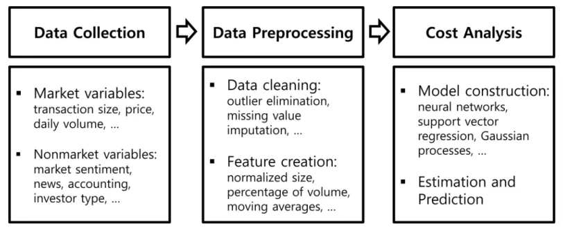
General procedures

First, we suggest the general procedure to find market impact costs by using nonparametric regression models before the descriptions of the simulation conducted in the current paper. The whole procedure is classified into three stages: data collection, data preprocessing, and cost analysis.Fig 1represents the summary of the whole procedure.

(6)

variables than may affect price or liquidity can also be useful as well as the traditional market variables because the nonparametric models do not require any restriction on the data and the general procedure of analyzing market impact costs using them will not be changed.

The gathered data from the first stage are preprocessed to make input variables that are used for learning process in the second stage. First, data cleaning processes such as outlier elim-ination and missing value imputation are conducted. Then, the input variables that will be used for the nonparametric models are derived from these cleaned data.

At the final stage, nonparametric models to estimate and predict market impact costs are constructed using the input variables created in the previous stage. In addition, any other anal-yses using the constructed model including testing statistical significance can be conducted at this stage.

Data description

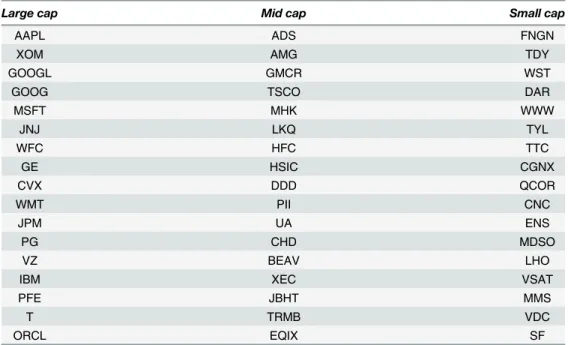
For simulating the proposed nonparametric approach, we gathered a single transaction data of the stocks of US equity markets from Bloomberg Terminal for the period from 2014/06/02 to 2014/06/26. We selected 17 representative firms that have large market capitals among each of S&P 500, S&P MidCap 400, and S&Ps SmallCap 600 indices. These indices are composed of large cap, mid cap, and small cap firms respectively. The tickers of the selected firms are pre-sented inTable 1.

The collected transactions data are classified into three data sets,large cap,mid cap, and

small capby their capitals; another data setall capincludes all transactions regardless of the market capital. For each size of capitals, the number of collected transactions are approximately 15 million, 2 million and 1 million forlarge cap,mid cap, andsmall cap, respectively. Thus the

all capdata set has approxiamtely 18 million transactions in total. The procedures in the fol-lowing sections will be applied commonly to all of those data sets.

Fig 1. Summary of the general procedure of nonparametric approach for market impact cost.

(7)

Creating and bucketing input variables

We made three key input variables,Size,Vol, andPOV, which are also used in I-star model [10,

11] and one output variable, the market impact cost. Considering that the I-star was originally applied to the daily-aggregated transactions, we slightly modified the input variables suitable for single high-frequent transactions. First, we define the market impact cost, denoted by

cost, as

cost¼side logðpt=p0Þ 10 4

ð12Þ

wheresideis 1 if a trade is a buy-initiated trade and−1 if a trade is a sell-initiated trade,p0is a mid-price just before the trade, andptis an executed price of the trade. Given thatcostis multi-plied by 104, the unit ofcostbecomes basis point (bp). Theﬁrst input variableSizeis the nor-malized trade size as follows:

Size¼ Vt

ATV ð13Þ

whereATVis the average trade volume of the previous day. In the original I-star model, the imbalanced trade size is normalized by 30-day average daily volume because the trade size itself is daily = aggregated. In our research, to apply the single transactions, we divide each trade size by the one-day average of the single trades of the previous day. The second input variableVol

is deﬁned as the 30-day volatility, and this value is the same with the original I-star model because volatility is the characteristic of each stock, unrelated to trade size or frequency.POV, the percentage of volume, in [11] is deﬁned asQ/VwhereQis the daily imbalanced size andV

is the total trade volume of that day. A single transaction may be affected by market liquidity more locally rather than the liquidity of the whole day. Thus we deﬁnePOVfor single

Table 1. Tickers of selected firms.

Large cap Mid cap Small cap

AAPL ADS FNGN

XOM AMG TDY

GOOGL GMCR WST

GOOG TSCO DAR

MSFT MHK WWW

JNJ LKQ TYL

WFC HFC TTC

GE HSIC CGNX

CVX DDD QCOR

WMT PII CNC

JPM UA ENS

PG CHD MDSO

VZ BEAV LHO

IBM XEC VSAT

PFE JBHT MMS

T TRMB VDC

ORCL EQIX SF

A total of 17ﬁrms with large market capitals among each of large, mid, and small cap indices by S&P are chosen.

(8)

transactions as

POV¼ Vt

Vtð t;tÞ

ð14Þ

whereVt(−τ,τ) is the total traded volume fromτminutes before the trade toτminutes after

the trade. Based on the previous study [7], we expected that the single transaction affects and is affected by the market within approximately 15 minutes and thus we decided thatτequals 15.

After creating input variables, we made three dimensional bins of input variables and bucketed the transactions into them. For each bin,Sizehas values of multiples of 0.01, i.e. 0,0.01,0.02,. . ._{, and}_Vol_{has values of multiple of 0.05.}_POV_{has the values of multiples of}

0.0002 for thelarge capdata set and multiples of 0.001 for the other types of data sets. Each transaction was bucketed to the bin with the nearest value. For example, a transaction from

mid capdata set with the input variables (Size,Vol,POV) = (0.0137,0.022,0.0038) was put to the bin with the values (Size,Vol,POV) = (0.01,0.02,0.004). The output,cost, of each bin is defined by the averagecostof transactions belonging to the bin.

Finally, we selected bins containing enough number of transactions. The criterion number will be different for data sets. We selected the bins containing more than 20, 30, 60, 100 trans-actions; the number of survived bins are 2931, 3356, 5706, 5119 forsmall cap,mid cap,large cap, andall cap, respectively.

Analyzing market impact costs

With respect to the bins of transactions to be used for the nonparametric machine learning models, we set 70% of survived bins as the training set and the remaining 30% as the test set for each data set. To find appropriate parameter sets of nonparametric models, we used 10-fold cross validation for the training set. After finding the parameter set, each model was retrained for the entire training set with the chosen parameter set and applied to the test set. As a parametric benchmark, we used I-star model with the same data sets. As described in Section, I-star model also requires finding certain parameters. We found the parameters for I-star model by grid search and 10-fold cross validation of the training set and applied it to the test set as the same with the nonparametric models. Finally, we applied Wilcoxon signed-rank test between each nonparametric model and the parametric benchmark for each capital size group to find whether the difference in performance between a nonparametric model and the bench-mark is significant.

Results

Predicting market impact costs

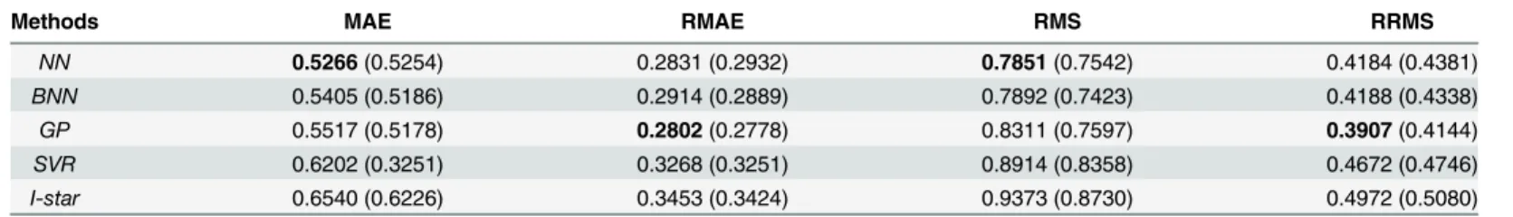
First, we applied the nonparametric machine learning models and the benchmark parametric model, I-star model, to the selected bins of each data set. To estimate the errors of the model, we used four different measures, mean absolute error (MAE), relative MAE (RMAE), root mean squared error (RMS), and relative RMS (RRMS). The summarized results are shown in Tables2–5.NN,BNN,SVR,GP, andI-starrefer to neural network, Bayesian neural network, support vector regression, Gaussian process, and I-star model, respectively.

(9)

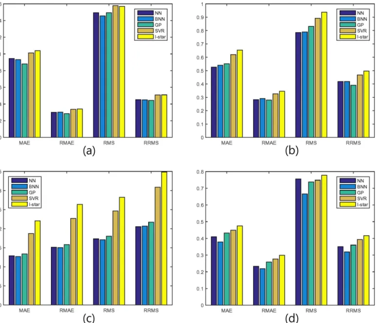
-0.005% to 15.03%. This phenomenon is more clarified byFig 2which represented the errors in the tables above.

In summary, we find that the three nonparametric models, neural network, Bayesian neural network, and Gaussian process, shows much better performances than the parametric

Table 2. Test errors of the nonparametric models and the parametric benchmark models forsmall capdata set.

Methods MAE RMAE RMS RRMS

NN 0.9445 (0.9910) 0.3006 (0.3175) 1.4945 (1.5305) 0.4535 (0.4990)

BNN 0.9310 (1.0025) 0.3023 (0.3204) 1.4559(1.5286) 0.4502 (0.4820)

GP 0.8794(0.8701) 0.2854(0.2716) 1.4945 (1.3950) 0.4442(0.4060)

SVR 1.0121 (1.0333) 0.3352 (0.3373) 1.5783 (1.5762) 0.5090 (0.5340)

I-star 1.0396 (1.0446) 0.3410 (0.3408) 1.5701 (1.5891) 0.5097 (0.5476)

Cross validation errors are also displayed in the parentheses. The best model for each error measure isboldfaced.

doi:10.1371/journal.pone.0150243.t002

Table 5. Test errors of the nonparametric models and the parametric benchmark models forall capdata set.

NN 0.4096 (0.3746) 0.4096 (0.2173) 0.7557 (0.6388) 0.3507 (0.3210)

BNN 0.3789(0.3683) 0.2182(0.2170) 0.6667(0.6251) 0.3192(0.3292)

GP 0.4327 (0.4059) 0.2586 (0.2519) 0.7383 (0.6598) 0.3601 (0.3576)

SVR 0.4488 (0.4256) 0.2766 (0.2710) 0.7485 (0.6840) 0.3933 (0.3964)

I-star 0.4747 (0.4517) 0.2989 (0.2931) 0.7784 (0.7029) 0.4163 (0.4149)

Table 4. Test errors of the nonparametric models and the parametric benchmark models forlarge capdata set.

NN 0.1287 (0.1283) 0.1515 (0.1506) 0.1732 (0.1738) 0.2051(0.2054)

BNN 0.1267(0.1280) 0.1502(0.1505) 0.1712(0.1735) 0.2066 (0.2061)

GP 0.1338 (0.1377) 0.1583 (0.1621) 0.1802 (0.1878) 0.2172 (0.2123)

SVR 0.1872 (0.1896) 0.2267 (0.2300) 0.2466 (0.2459) 0.3085 (0.3112)

I-star 0.2203 (0.2229) 0.2635 (0.2661) 0.2823 (0.2823) 0.3484 (0.3503)

Table 3. Test errors of the nonparametric models and the parametric benchmark models formid capdata set.

NN 0.5266(0.5254) 0.2831 (0.2932) 0.7851(0.7542) 0.4184 (0.4381)

BNN 0.5405 (0.5186) 0.2914 (0.2889) 0.7892 (0.7423) 0.4188 (0.4338)

GP 0.5517 (0.5178) 0.2802(0.2778) 0.8311 (0.7597) 0.3907(0.4144)

SVR 0.6202 (0.3251) 0.3268 (0.3251) 0.8914 (0.8358) 0.4672 (0.4746)

I-star 0.6540 (0.6226) 0.3453 (0.3424) 0.9373 (0.8730) 0.4972 (0.5080)

(10)

benchmark while support vector regression model performs slightly better than the benchmark and worse than the other nonparametric models in general. In some measures such as RMS, support vector regression performs slightly worse than the benchmark model forsmall capdata set.

To validate the proposed approach, in addition, we applied the Wilcoxon signed-rank test to each pair of the instance-wise test errors of one nonparametric model and the benchmark parametric model for each error measure. The p-values obtained by normal approximation of the Wilcoxon signed-rank test and all of them were smaller than 0.05, which is usually consid-ered as a critical value of the statistical significance. Even though the averaged RMS of SVR

Fig 2. Test errors of the nonparametric machine learning models and the parametric benchmark.(a)small capdata set (b)mid capdata set (c)large capdata set (d)all capdata set.

(11)

prediction is larger than the benchmark, the predicted performance of SVR was judged signifi-cantly better than the parametric benchmark by the Wilcoxon signed-rank test.

Discussion

In this study, we introduced the nonparametric approaches to estimate and predict market impact costs and applied them to US stock markets with the three input variables used in I-star model, the parametric benchmark. This study has several features. First, four state-of-the-art nonparametric machine learning models including NN, BNN, GP, and SVR have been applied to the task of analyzing market impact cost, whereas the previous studies were focused on only parametric models. The nonparametric machine learning approaches have advantages in both prediction performance and versatility in the number of input variables. Second, the data set used in this study was highly extensive. A total 17 firms were selected from each indices of large, mid, and small cap firms, while the previous studies mostly focused on the large cap firms. The total amount of transactions used in this study exceeded 18 million. Finally, the market impact prediction in this paper used independent variables from single transactions. Thus, this prediction has the advantages to be applied to technological high-frequency trades compared with previous studies that analyzed only large trades.

As a result of the experiments performed in this study, the performances of nonparametric machine learning models mostly overwhelmed the benchmark model with the same input vari-ables for all kinds of firm sizes and all error measures. In particular, BNN, NN, and GP showed noticeably better performances, whereas SVR sometimes performed worse than or comparably to the benchmark model. The statistical significance of the predictive powers of nonparametric approaches was also validated by applying the Wilcoxon signed rank test to the test error.

However, one of the limitations of the nonparametric machine learning approaches is that they cannot directly separate the market impact cost into permanent and temporary cost, whereas some parametric models can. Considering that the total, or instantaneous impact pri-marily affects the price at which the transaction occurs, an indirect way to analyze the perma-nent or temporary portion of it using nonparametric models can be helpful in analyzing market characteristics. In addition, though the nonparametric models usually performed better than did the parametric benchmark with the same input variables, the magnitude of perfor-mance difference can be changed if the period or the selected firms vary.

This study implies possibilities to be extended on some points. First, the nonparametric machine learning models has the advantage over parametric models in that the input variables can be added freely without any limitations. Thus, studies related to the nonmarket variables affecting the market impact can be easily incorporated into nonparametric models rather than parametric ones which are formed with a priori fixed input variables. Next, several parametric models explain the market impact cost. However, they are difficult to compare because their input variables are varied, as is their number. In such cases, a nonparametric machine learning model with the same inputs as the parametric models can provide a performance benchmark. Finally, developing hybrid models of nonparametric and parametric ones that comprise the permanent and temporary portions of the market impact cost as well as that maintain the extendability and the performance level remains a future research topic related to this study.

Acknowledgments

(12)

Author Contributions

Conceived and designed the experiments: SP JL YS. Performed the experiments: SP JL YS. Ana-lyzed the data: SP JL YS. Contributed reagents/materials/analysis tools: SP JL YS. Wrote the paper: SP JL YS.

References

1. Lillo F, Farmer JD, Mantegna RN. Econophysics: Master curve for price-impact function. Nature. 2003; 421(6919): 129–130. doi:10.1038/421129aPMID:12520292

2. Gabaix X, Gopikrishnan P, Plerou V, Stanley HE. A theory of power-law distributions in financial market fluctuations. Nature. 2003; 423(6937): 267–270. doi:10.1038/nature01624PMID:12748636

3. Bouchaud JP, Gefen Y, Potters M, Wyart M. Fluctuations and response in financial markets: the subtle nature of’random’price changes. Quantitative Finance. 2004; 4(2): 176–190. doi:10.1080/

14697680400000022

4. Plerou V, Gopikrishnan P, Gabaix X, Stanley HE. Quantifying stock-price response to demand fluctua-tions. Physical review. E, Statistical, nonlinear, and soft matter physics. 2002; 66(2). doi:10.1103/ PhysRevE.66.027104PMID:12241320

5. Almgren R, Thum C, Hauptmann E, Li H. Direct estimation of equity market impact. Risk. 2005; 18(7): 58–62.

6. Kato T. An optimal execution problem with market impact. Finance and Stochastics. 2014; 18(3): 695–

732. doi:10.1007/s00780-014-0232-0

7. Frino A, Bjursell J, Wang GH, Lepone A. Large trades and intraday futures price behavior. Journal of Futures Markets. 2008; 28(12): 1147–1181. doi:10.1002/fut.20366

8. Bershova N, Rakhlin D. The non-linear market impact of large trades: Evidence from buy-side order flow. Quantitative Finance. 2013; 13(11): 1759–1778. doi:10.1080/14697688.2013.861076 9. Huberman G, Stanzl W. Optimal liquidity trading. Review of Finance. 2005; 9(2): 165–200. doi:10.

1007/s10679-005-7591-5

10. Kissell R, Glantz M, Malamut R. Optimal trading strategies: quantitative approaches for managing mar-ket impact and trading risk. Amacom; 2003.

11. Kissell R. The science of algorithmic trading and portfolio management. Academic Press; 2013. 12. Bikker JA, Spierdijk L, Van Der Sluis PJ. Market impact costs of institutional equity trades. Journal of

International Money and Finance. 2007; 26(6): 974–1000. doi:10.1016/j.jimonfin.2007.01.007 13. Bikker JA, Spierdijk L, Hoevenaars RP, Van der Sluis PJ. Forecasting market impact costs and

identify-ing expensive trades. Journal of Forecastidentify-ing. 2008; 27(1): 21–39. doi:10.1002/for.1052

14. Chen WH, Shih JY, Wu S. Comparison of support-vector machines and back propagation neural net-works in forecasting the six major Asian stock markets. International Journal of Electronic Finance. 2006; 1(1): 49–67. doi:10.1504/IJEF.2006.008837

15. Son Y, Noh DJ, Lee J. Forecasting trends of high-frequency KOSPI200 index data using learning clas-sifiers. Expert Systems with Applications. 2012; 39(14): 11607–11615. doi:10.1016/j.eswa.2012.04. 015

16. Ticknor JL. A Bayesian regularized artificial neural network for stock market forecasting. Expert Sys-tems with Applications. 2013; 40(14): 5501–5506. doi:10.1016/j.eswa.2013.04.013

17. Liao SH, Chou SY. Data mining investigation of co-movements on the Taiwan and China stock markets for future investment portfolio. Expert Systems with Applications. 2013; 40(5): 1542–1554. doi:10. 1016/j.eswa.2012.08.075

18. Hutchinson JM, Lo AW, Poggio T. A nonparametric approach to pricing and hedging derivative securi-ties via learning networks. The Journal of Finance. 1994; 49(3): 851–889. doi:10.1111/j.1540-6261. 1994.tb00081.x

19. Han GS, Lee J. Prediction of pricing and hedging errors for equity linked warrants with Gaussian pro-cess models. Expert Systems with Applications. 2008 35(1): 515–523. doi:10.1016/j.eswa.2007.07. 041

20. Park H, Kim N, Lee J. Parametric models and non-parametric machine learning models for predicting option prices: Empirical comparison study over KOSPI 200 Index options. Expert Systems with Applica-tions. 2014; 41(11): 5227–5237. doi:10.1016/j.eswa.2014.01.032

(13)

22. Gündüz Y, Uhrig-Homburg M. Predicting credit default swap prices with financial and pure data-driven approaches. Quantitative Finance. 2011; 11(12): 1709–1727. doi:10.1080/14697688.2010.531041 23. Kim KJ, Ahn H. A corporate credit rating model using multi-class support vector machines with an

ordi-nal pairwise partitioning approach. Computers & Operations Research. 2012; 39(8): 1800–1811. doi: 10.1016/j.cor.2011.06.023

24. Kim SH, Noh HJ. Predictability of interest rates using data mining tools: a comparative analysis of Korea and the US. Expert Systems with Applications. 1997; 13(2): 85–95. doi:10.1016/S0957-4174 (97)00010-9

25. Cao LJ, Tay FEH. Support vector machine with adaptive parameters in financial time series forecasting. Neural Networks, IEEE Transactions on. 2003; 14(6): 1506–1518. doi:10.1109/TNN.2003.820556 26. Osuna E, Freund R, Girosi F. An improved training algorithm for support vector machines. Proceedings

of the 1997 IEEE Workshop of Neural Networks for Signal Processing: IEEE; 1997.

27. Bhattacharyya S, Pictet OV, Zumbach G. Knowledge-intensive genetic discovery in foreign exchange markets. Evolutionary Computation, IEEE Transactions on. 2002; 6(2): 169–181. doi:10.1109/4235. 996016

28. Rosenblatt F. Principles of Neurodynamics: Perceptrons and the Theory of Brain Mechanisms. Wash-ington DC: Spartan; 1962.

29. Rumelhart DE, Hinton GE, Williams RJ. Learning internal representations by error propagation. CALI-FORNIA UNIV SAN DIEGO LA JOLLA INST FOR COGNITIVE SCIENCE. 1985

30. MacKay DJ. Bayesian interpolation. Neural computation.1992; 4(3): 415–447. doi:10.1162/neco. 1992.4.3.415

31. Foresee F.D, Hagan MT. Gauss-Newton approximation to Bayesian learning. Proceedings of the 1997 international joint conference on neural networks. Piscataway: IEEE; 1997; 3: 1930–1935.

32. Cressie NA. Statistics for spatial data. Wiley: New York; 1993.

33. Rasmussen CE. Evaluation of Gaussian processes and other methods for non-linear regression. Doc-toral dissertation, University of Toronto; 1996.

34. Rasmussen CE, Williams CKI. Gaussain Processes for Machine Learning. MIT press; 2006. 35. Drucker H, Burges CJ, Kaufman L, Smola A, Vapnik V. Support vector regression machines. in: