STATE-SPACE APPROACH FOR THE ANALYSIS OF SOIL
WATER CONTENT AND TEMPERATURE
IN A SUGARCANE CROP
Durval Dourado-Neto3,6; Luís Carlos Timm1*; Julio Cesar Martins de Oliveira1,4; Klaus
Reichardt1,2,6; Osny Oliveira Santos Bacchi1,6; Tania Toyomi Tominaga1,4; Fabio Augusto Meira
Cássaro1,3,5
1
Laboratório de Física do Solo - CENA/USP, C.P. 96 - CEP: 13400-970 - Piracicaba, SP.
2
Depto. de Ciências Exatas - ESALQ/USP, C.P. 9 - CEP: 13418-970 - Piracicaba, SP.
3
Depto. de Produção Vegetal - ESALQ/USP.
4
Bolsista da FAPESP.
5
Bolsista do CAPES.
6
Bolsista do CNPq.
*e-mail: lctimm@carpa.ciagri.usp.br
ABSTRACT: The state-space approach is used to describe surface soil water content and temperature behaviour, in a field experiment in which sugarcane is submitted to different management practices. The treatments consisted of harvest trash mulching, bare soil, and burned trash, all three in a ratoon crop, after first cane harvest. One transect of 84 points was sampled, meter by meter, covering all treatments and borders. The state-space approach is described in detail and the results show that soil water contents measured along the transect could successfully be estimated from water content and temperature observations made at the first neighbour.
Key words: soil water, soil temperature, state-space, transect
A ABORDAGEM DE ESTADO-ESPAÇO NA ANÁLISE DO CONTEÚDO DE ÁGUA E TEMPERATURA DO SOLO EM UMA CULTURA DE CANA
RESUMO: Para estudar o comportamento do conteúdo de água e da temperatura na camada superficial do solo, a abordagem “state-space” foi empregada em dados obtidos em uma cultura de cana submetida à práticas distintas de manejo. Os tratamentos constaram de cobertura morta com palha (e ponteiros), solo nu e palha queimada, todos no início da primeira soca. As amostragens foram realizadas em uma transeção de 84 pontos, metro a metro, cobrindo todos os tratamentos e bordaduras. A metodologia “state-space” é descrita em detalhe e os resultados mostram que o conteúdo de água no solo pode ser estimado com sucesso a partir de dados de conteúdo de água e de temperatura observados no primeiro vizinho.
Palavras-chave: água no solo, temperatura do solo, estado-espaço, transeção
INTRODUCTION
Several physical, chemical and biological phenomena are observed in a form that leads to a numerical quantification in a sequence, distributed in time, called time series. The simplest form used to define a time series Zt; t=1,2,..., is by understanding Zt as a set of discrete observations, obtained in equal time intervals and that present a serial dependence among themselves. This concept, although simple, gives a special emphasis to the “Time Series Analysis” as a well defined area inside Statistics, since independent and identically distributed data are clearly discarded, in contrast
among observations and disregard their location intra-field, these newly applied methods in soil science, take advantage of the spatial dependence making use of the location of each observation. Several statistical tools, like autocorrelation function, semivariograms and state-space, have been used more recently to evaluate the structure of spatial distributions of soil properties (Wendroth et al., 1997; Hui et al., 1998). According to Bresler et al. (1981), research of the last two decades has focused the study of soil spatial variability with the aim of better understanding the processes that influence the variability of crop production. Nielsen & Alemi (1989) comment that in several reports using classical statistics, observations within and between treatments are not always independent, making the used statistical design inadequate.
Vauclin et al. (1982) studied the variability of soil water and temperature using an autoregressive model of first order. Shumway (1988) states that the state-space analysis is a special kind of autoregressive model. Some of the early applications of the state-space approach are given in Morkoc et al. (1985) and Wendroth et al. (1992). In this report, we present a state-space analysis of sets of soil water content and of soil temperature data, collected in a sugarcane field, submitted to different management treatments. It is intended to contribute for a better understanding of the relation between water and temperature behavior in the soil.
THEORETICAL ASPECTS
In the state-space analysis, the state of a system, of a variable, or of a set of variables measured at a location i, is related to the state of the same and other variables, at location i-h, where h=1,2,3,...,n, called the lag between neighbour observations. This autoregressive model is used for several types of prediction (and forecast) based on a space or time series, to identify coefficients that join these state systems (Wendroth et al., 1997).
The basic equation is called state equation, which for h=1 can be written as:
Xi = φ Xi-1 + Wi (1)
where Xi is the state vector (of a set of p
variables) at location i; φ is a p x p matrix of state
coefficients, which indicate the measure of the
regression; and Wi are noises of the system for
i=1,2,3,...,n, assumed to have zero mean, not
correlated and normally distributed. This is the usual structure of a common autoregressive
model, in which the coefficients of the matrix φ
could be calculated by multiple regression, taking
Xi as the dependent variable and X i-1 as
independent one. In the state-space model, however, the true state of the variable, or of the state vector, is considered “embedded” in the following observation equation:
Yi = Ai Xi + Vi (2)
where the observation vector Yi is related to the
state vector Xi by an observation matrix Ai (unit
matrix, p x p) and observation noises Vi, of zero
mean, not correlated and normally distributed.
The noises Wi and Vi are considered independent
of each other, in other words, what is measured does not have to be taken as true, but can be considered as an indirect measurement, reflecting the true state of the variable added to the noise (Wendroth et al, 1997).
Considering the case of this study, Xi is
the soil water content θi (cm3.cm-3) and the soil
temperature Ti (oC), and equation (1) can be
written in the following matrix form:
(1a) W W T
T Ti
i 1 -i 1 i 22 21 12 11 i i + θ × φ φ φ φ =
θ − θ
The state coefficients φk,j and noises of
equation (1a) are estimated through a recursive procedure given by Shumway & Stoffer (1982). They are optimised using the Kalman (1960) filter, with an iterative algorithm. This filter is a recursive procedure to find optimised estimators for the state vector at position i. Motta & Hotta (1998) state that this filter is frequently used in engineering (Mine, 1984; Gomes & Mine, 1989; 1991; Alves et al., 1991) since it permits the estimation of the state vector with its constant renewal as new observations are obtained, the actual value of the state vector being of most interest.
Equation (2) can also be written as:
(2a) V V T 1 0 0 1
T Ti
i i i o i o i + θ × = θ θ
in which θio e T i
o are observed values at location
uncertainties of θ and T and to the influence of other not measured variables that can affect them (Morkoc et al., 1985).
MATERIAL AND METHODS
Soil water content (θ) and soil
temperature (T) data were collected in a field
study carried out at Piracicaba, SP, Brazil (22o 42’
S and 47o 38’ W) on an area of a dark red
latosol, called “terra roxa estruturada” (Rhodic Kandindox) (Figure 1). The crop was planted in October 1997, harvested in October 1998, and after this the soil temperature and moisture study began, using the first ratoon crop. Three management treatments were compared: i. mulching with trash (cane tips and straw from the
last harvest, T1 and T2); ii. bare soil between rows
(T3); and iii. soil surface with the residues left by
the traditional practice of straw burning before
harvest (T4). The treatments T1 and T2 are similar
in respect to the mulching with trash, and therefore replicates in terms of this soil temperature study, being different only in terms
of 15N label which was used in an additional
organic matter residue study.
Soil temperatures were measured with digital stick thermometers, introduced into the soil down to three depths: 3, 6 and 9 cm. Readings were made after equilibrium (about 3 minutes). In this study, the average of the three depths was used. Soil water contents were obtained using a single gamma-neutron surface probe, model CPN, MC-3. This gauge operates in such a way that water contents are measured by neutron moderation, sampling a semi-sphere of radius of
about 15 cm, so that θ measurements are
averages of the 0 – 15 cm soil layer.
Data of θ and T were simultaneously
collected, at noon (11:00 am to 12:00), along a 84 point transect that covers all treatments and borders. Data collected on Nov. 1998 were analysed through the state-space approach, using the software ASTSA (Applied Statistical Time Series Analysis), developed by Shumway (1988). According to Hui et al. (1998), if for the state-space analysis data are transformed by:
xi=
[
Xi-(
m-2s)
]
/4s (3)the state coefficients φk,j in equation (1) will have
magnitudes directly proportional to the contribution of each respective state variable used
in the analysis. Transformed values xi have a
mean equal to 0.5. In equation (3), m is the mean
of Xi and s the standard deviation.
RESULTS AND DISCUSSION
Soil water content and temperature data used in this study, collected along the 84 point transect, are shown in Figure 2. The temperature data reflect visually the effect of the treatments on the average soil temperature of the surface
layer (3 to 9 cm), treatments T1 and T2 presenting
much lower temperatures (overall average of
23.2oC) due to the presence of the mulch (trash
= tips + straw, 127 kg.ha-1 of dry matter); T
3 with bare soil surface presenting an average of
30.1oC; and T
4, the burned treatment, with an
average of 28.3oC. The sharp temperature
differences are due to the fact that they were measured two weeks after harvest of the first crop, when the ratoon crop was starting to sprout, so that the field was completely exposed to sunshine on November 20, 1998, a late spring day, after a sequence of 6 days without rainfall.
Soil water content data, collected at the same day, present an inverse relation, the
mulched treatments T1 and T2 show relatively
higher water contents in relation to the bare T3
Figure 1 - Schematic experimental design showing
the 15 cane lines, 100 m long,
indicating the 3 central lines that
received 15N labeled fertilizer. B=
border; T= treatment; R= replicate.
B T3 R3 T3 R1 T3 R2 T3 R4 B T2 R1 T2 R3 T2 R4 T2 R2 B T1 R1 T1 R4 T1 R2 T1 R3 B T4 R1 T4 R2 T4 R3 T4 R4 B
→ crop line
16 m
100 m 84 m
4 m
1,4 m
and the burned T4 treatments. This is demonstrated
in Figure 3, which presents a correlation (R2 =
0.4491, significant at the level of 5 %) between soil
temperature T and soil water content θ. The
negative slope of the relation expresses the inverse
relation between T and θ.
The crosscorrelogram of Figure 4 shows the strong spatial dependence of the variables T
and θ, which is significant at the 5 % probability
level, up to 7 or more lags. The semivariograms (gamma h) presented in Figures 5 and 6 show also a clear spatial dependence of both variables, since values of gamma increase with the
tendency of reaching the variance (s2),which
represent the variability of the total population disregarding their locations.
The state-space analysis applied to soil water content and temperature, is presented in Figures 7 and 8 respectively, after transforming the data according to equation (3). The obtained matrix coefficients were:
θi= 0.881 θi-1 + 0.1148 Ti-1 + Wθi
Ti= 0.0615 θi-1 + 0.9272 Ti-1 + WTi
The shaded area of Figures 7 and 8 represent the fiducial limits considering ± one
standard deviation (s). For θ and T the average
values of s given by the ASTSA programm were 0.0937 and 0.0732, respectively.
Analysing equation (1b), it can be seen
that θ at location i-1 contributes with 88.1% to the
estimate of θ in i, while T at i-1 contributes with
11.5%, showing that the contribution of θ of the
first neighbour is more significant than that of T.
Morkoc et al. (1985) verified a contribution of θi-1
and T i-1 of 98.9 and 0.3%, respectively, on the
estimation of θi.
For the case of temperature estimation
(Figure 8), equation (1b) shows that θi-1
contributes with 6.2% in the estimate of the
temperature at point i. On the other hand, T i-1
contributes with 92.7%. Morkoc et al. (1985) found, in this case, contributions of 11.0 and 96.4%. It is important to note that these authors did not transform their data according to equation (3), and that for their case, it is more difficult to estimate the contributions of each variable.
The above shown state-space analysis is the first performed on soil spatial data in Brazil. One objective is its introduction into the Brazilian literature and, as already said, contribute for a
better understanding of the relation between θ
and T. Figures 9 and 10 indicate how well the state-space model estimates the variables under
study. This can also be seen in the already discussed Figures 7 and 8, in which most of the observed values fall inside the fiducial limit of ± one s.
Data show clearly, mainly Figure 3, the
inverse relation between T and θ. Added to
(Figures 4, 5 and 6) this, there is a strong spatial dependence, which justifies the application of the state-space methodology. Therefore, soil water contents could be well estimated from neighbour values, including information on temperature. Since temperature measurements are easier and quicker than those of soil water content, the analysis here presented suggests that the one measurement could, in many situations, replace the other. Relating soil properties at sites i to properties at sites i-h is also of practical importance, mainly to farmers. In this study, the lag of 1m is small for practical pourpouses, it is however very important to better understand how far one property is affected by its neighbour, and so recognise management measures that would lead to increased yield. Precision agriculture is one of the recent fields very interested in these aspects.
Figure 2 - Soil temperature and water content distributions, meter by meter, along the 84 point transect, at noon (11:00
12:00) on Nov. 20, 1998. B=border; T1
and T2= trash mulching; T3= bare soil;
T4= burned trash.
10 20 30 40 50 60 70 80
0.20 0.25 0.30 0.35 0.40
T4
T1 T2
T3 B B B B
B
1
S o i l w a t e r c o n t e n t (cm
3.cm -3)
Soil water content
10 20 30 40 50 60 70 80
22 24 26 28 30 32 34
Temperature
S o i l t e m p e r a t u r e (
oC)
L o c a t i o n s i n t h e t r a n s e c t (m)
0 5 10 15 20 2
4 6 8 10 12
2 4 6 8 10 12 V a r i a n c e (s2) = 10.93
G a m m a (h) s o i l t e m p e r a t u r e
D i s t a n c e, l a g (m)
0 5 10 15 20
0.0006 0.0008 0.0010 0.0012 0.0014 0.0016 0.0018 0.0020
Variance(s2) = 0.001763
G a m m a (h) s o i l w a t e r c o n t e n t
D i s t a n c e, l a g (m)
0.15 0.20 0.25 0.30 0.35 0.40
22 24 26 28 30 32 34
θ
R 2 = 0.4491
Τ = − 52.764 θ + 41.235
S o i l t e m p e r a t u r e T (
oC)
S o i l w a t e r c o n t e n t ( cm3.cm-3)
Figure 6 - Soil temperature semivariogram, estimated using data of Figure 2. Figure 3 - Correlation between soil temperature
and water content data of Figure 2. Figure 4 - Crosscorrelogram between soil temperature and water content data
of Figure 2.
Figure 5 - Soil water content semivariogram, estimated using data of Figure 2.
-10 -5 0 5 10
-0.8 -0.6 -0.4 -0.2 0.0 0.2 0.4 0.6 0.8
Significancy level (95% = 0.213)
C r o s s c o r r e l a t i o n c o e f f i c i e n t (R)
0.0 0.2 0.4 0.6 0.8 1.0 1.2 0.0
0.2 0.4 0.6 0.8 1.0 1.2
1:1 line R 2 = 0.9557
T r a n s f o r m e d e s t i m a t e d s o i l w a t e r c o n t e n t
T r a n s f o r m e d o b s e r v e d s o i l w a t e r c o n t e n t
Figure 7 - State-space analysis of transformed
(equation 3) soil water content φ data
of Figure 2.
Figure 8 - State-space analysis of transformed (equation 3) soil temperature T data of Figure 2.
Figure 9 - Correlation between transformed (equation 3) estimated and observed soil water content data.
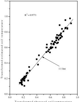
Figure 10 - Correlation between transformed (equation 3) estimated and observed soil temperature data.
0.0 0.2 0.4 0.6 0.8 1.0
0.0 0.2 0.4 0.6 0.8 1.0 1.2
1:1 line R 2 = 0.9771
T r a n s f o r m e d e s t i m a t e d s o i l t e m p e r a t u r e
T r a n s f o r m e d o b s e r v e d s o i l t e m p e r a t u r e
10 20 30 40 50 60 70 80
0.0 0.2 0.4 0.6 0.8 1.0 1.2
Ti = 0.0615 θi-1 + 0.9272 Ti-1 + WTi T estimated + s
T estimated - s
10 20 30 40 50 60 70 80
0.0 0.2 0.4 0.6 0.8 1.0 1.2
T observed
T r a n s f o r m e d s o i l t e m p e r a t u r e ( T)
L o c a t i o n s o n t h e t r a n s e c t
10 20 30 40 50 60 70 80
0.0 0.2 0.4 0.6 0.8 1.0 1.2
2
T estimated from equation
10 20 30 40 50 60 70 80
-0.2 0.0 0.2 0.4 0.6 0.8 1.0 1.2
θ observed
T r a n s f o r m e d s o i l w a t e r c o n t e n t (
θ
)
L o c a t i o n s o n t h e t r a n s e c t
10 20 30 40 50 60 70 80
-0.2 0.0 0.2 0.4 0.6 0.8 1.0 1.2
2
θi = 0.881θi-1 + 0.1148 Ti-1 + Wθi
θ estimated from equation θ estimated + s
REFERENCES
ALVES, M.H.; MAGALHÃES, P.C.; KELMAN, J. Previsão em tempo real de vazão associada a uma incerteza e utilizando técnica de filtragem de erros. In: SIMPÓSIO BRASILEIRO DE RECURSOS HÍDRICOS, 9., Rio de Janeiro,1991. Anais. São Paulo: ABRH, 1991. p.111-123 BRESLER, E.; DASBERG, S.; RUSSO, D.; DAGAN,
G. Spatial variability of crop yield as a stochastic soil process. Soil Science Society of America Journal, v.45, p.600-605, 1981.
GOMES, J.; MINE, M.R.M. Estimativa do hidrograma unitário através da técnica do filtro de Kalman. In: SIMPÓSIO BRASILEIRO DE RECURSOS HÍDRICOS, 8., Foz do Iguaçu, 1989. Anais. São Paulo: ABRH,. p.92-100.
GOMES, J.; MINE, M.R.M. Estimativa dos parâmetros de um modelo autoregressivo através da técnica do filtro de Kalman. In: SIMPÓSIO BRASILEIRO DE RECURSOS HÍDRICOS, 9., Rio de Janeiro, 1991. Anais. São Paulo: ABRH, 1991. p.428-435.
HUI, S.; WENDROTH, O.; PARLANGE, M.B.; NIELSEN, D.R. Soil variability: infiltration relationships of agroecosystems. Journal of Balkan Ecology, v.1, n.2, p.21-40, 1998. KALMAN, R.E. A new approach to linear filtering
and prediction theory. Journal de Basic Engineering, v.8, p.35-45, 1960.
MINE, M.R.M. Modelos estocásticos lineares para previsão de cheias em tempo real. São Paulo, 1984. 127p. Dissertação (Mestrado) -Universidade de São Paulo.
MORKOC, F.; BIGGAR, J.W.; NIELSEN, D.R.; ROLSTON, D.E. Analysis of soil water content and temperature using State-space approach. Soil Science Society of America Journal, v.49, p.798-803, 1985.
MOTTA, A.C.O.; HOTTA, L.K. Utilização do filtro de Kalman em modelos estatísticos. UNICAMP, Instituto de Matemática, Estatística e Computação Científica, 1998. 71p.
NIELSEN, D.R.; ALEMI, M.H. Statistical opportunities for analyzing spatial and temporal heterogeneity of field soils. Plant and Soil, v.115, p.285-296, 1989.
SHUMWAY, R.H.; STOFFER, D.S. An approach to time series smoothing and forecasting using the EM algorithm. Journal of Time Series Analysis, v.3, p.253-264, 1982.
SHUMWAY, R.H. Applied statistical time series analysis. Englewood Cliffs: Prentice Hall, 1988. SOUZA, R.C. Modelos estruturais para previsão de séries temporais: abordagem clássica e bayesiana. In: COLÓQUIO BRASILEIRO DE MATEMÁTICA, 17., Rio de Janeiro, 1989. Anais. Rio de Janeiro: IMPA, 1989. 171p.
VAUCLIN, M.; VIEIRA, S. R.; BERNARD, R.; HATFIELD, J.L. Spatial variability of surface temperature along two transects of a soil. Water Resources Research, v.18, p.1677-1686, 1982. WENDROTH, O., REYNOLDS, W. D., VIEIRA, S. R., REICHARDT, K., WIRTH, S. Statistical approaches to the analysis of soil quality data. In: GREGORICH, E.G.; CARTER, M.R. (Ed.) Soil quality for crop production and ecosystem health. Amsterdam: Elsevier, 1997. p.247-276. WENDROTH, O.; AL OMRAN, A.M.; KIRDA, K.; REICHARDT, K.; NIELSEN, D.R. State-space approach to spatial varialility of crop yiel. Soil Science Society of America Journal, v.56, p.801-807, 1992.