Measuring higher order optical aberrations of the human eye: techniques and applications

Measuring higher order optical

aberrations of the human eye:

techniques and applications

1_{Grupo de Óptica, Instituto de Física de São Carlos, Universidade de São Paulo,}

São Carlos, SP, Brasil

2_{Departamento de Matemática, Universidade Estadual de Maringá,}

Maringá, PR, Brasil L. Alberto V. Carvalho1_,

J.C. Castro1 _and

L. Antonio V. Carvalho2

Abstract

In the present paper we discuss the development of “wave-front”, an instrument for determining the lower and higher optical aberrations of the human eye. We also discuss the advantages that such instrumenta-tion and techniques might bring to the ophthalmology professional of the 21st century. By shining a small light spot on the retina of subjects and observing the light that is reflected back from within the eye, we are able to quantitatively determine the amount of lower order aberra-tions (astigmatism, myopia, hyperopia) and higher order aberraaberra-tions (coma, spherical aberration, etc.). We have measured artificial eyes with calibrated ametropia ranging from +5 to -5 D, with and without 2 D astigmatism with axis at 45º and 90º. We used a device known as the Hartmann-Shack (HS) sensor, originally developed for measuring the optical aberrations of optical instruments and general refracting surfaces in astronomical telescopes. The HS sensor sends information to a computer software for decomposition of wave-front aberrations into a set of Zernike polynomials. These polynomials have special mathematical properties and are more suitable in this case than the traditional Seidel polynomials. We have demonstrated that this tech-nique is more precise than conventional autorefraction, with a root mean square error (RMSE) of less than 0.1 µm for a 4-mm diameter pupil. In terms of dioptric power this represents an RMSE error of less than 0.04 D and 5º for the axis. This precision is sufficient for customized corneal ablations, among other applications.

Correspondence

L. Alberto V. Carvalho Grupo de Óptica, IFSC, USP 13560-900 São Carlos, SP Brasil

E-mail: lavcf@ifsc.sc.usp.br Research partially supported by FAPESP (Nos. 01/03132-8 and 00/06810-4). L. Antonio V. Carvalho is partially supported by CNPq (No. 304041/85-8).

Received June 28, 2001 Accepted June 10, 2002

Key words

·Optical aberrations ·Corneal topography ·Zernike polynomials ·Refractive surgery

Introduction

The ophthalmology professional of the 21stcentury is living a silent revolution, one which started at the University of Heidelberg (1994) with the Ph.D. thesis of Liang (1). Many scientists throughout the history of physiological optics have attempted to pre-cisely measure the optical aberrations of the

a hyperope. This device was the first qualita-tive refractor and became known as Schei-ner’s disc. After Scheiner, many scientists attempted to construct more precise refrac-tors. Tscherning (4) in 1894 used a four-dimensional spherical lens with a grid pat-tern on its surface to project a regular patpat-tern on the retina (Figure 2). He would then ask the patient to sketch drawings of the pattern. Depending on the pattern’s distortion, Tscherning was able to obtain a semiquanti-tative measurement of the patient’s aberra-tions. It was only at the beginning of the 1960s that Howland (5) devised a quantita-tive version of the Tscherning aberroscope by attaching an imaging system and imple-menting rigorous mathematical analysis of the collected data. Of course, low resolution quantitative systems (autorefractors) have been developed in parallel throughout the last quarter of the last century. We will not discuss the principle of these instruments here, which has been recently reported else-where (6-9), but we will compare the preci-sion of our results with those of autorefractors in general.

The instruments devised by Scheiner, Tscherning and later by Howland, all had a specific disadvantage. They were developed in a “non-computerized age”. Although there were computers back in the 1960s, the mi-crocomputer “revolution” started only in the mid-1980s. The same occurred with the de-vices for measuring corneal curvature (video-keratoscopes). Although Plácido (10)

devel-oped the technique still used nowadays more than a century ago other devices with magni-fying optics and photographic cameras were only possible later in the 20thcentury. These improvements culminated in the develop-ment of well-known keratometers and the photokeratoscope. But these were still lim-ited techniques. The keratometer is still used today, but it only measures the steepest and the flattest meridians at the central 3 mm of the cornea; the photokeratoscope photo-graphs had to be developed and analyzed manually, a process that could take hours, if not days. And even after a careful analysis, few techniques were available for displaying these results in a comprehensive and com-pact fashion. There were no fast methods for Scientific Visualization (11) (a term refer-ring to a relatively new field in computer graphics, initiated in the mid-1980s, with the objective of developing more didactic tech-niques for visual presentation and analysis of scientific data). Since the mid-1980s, with the microcomputer “revolution”, computer power became accessible enough so as to be incorporated into traditional photokerato-scopes. Thus, the photokeratoscope became the modern computerized videokeratoscope, which is an example of the improvement allowed by the integration of computers and medical devices. The photographic cameras were replaced by modern semiconductor charge coupling devices (CCD) and the tire-some analysis of the Plácido images was replaced by fast and semiautomated image processing algorithms (12,13) and sophisti-cated mathematical models of the human cornea (14,15). Nowadays the whole pro-cess of corneal analysis takes only a few seconds and at the end the eye-care profes-sional may have a multitude of visualization options at a click of the mouse, with the aid of special tools, such as indexes for kerato-conus screening(16,17), contact lens fitting modules (18) and special displays of corneal parameters (19). These displays may go from simple corneal slices, difference maps for Light bundle

Grid mask Figure 2. The Tscherning

aber-roscope.

Paraxial

Two retinal points

Eye with aberration Figure 1. The principle of

pre- and postsurgical analysis, up to rotating three-dimensional corneal maps.

It is our very strong belief that the refrac-tion techniques available nowadays have many limitations, analogous to the photo-keratoscopes back in the 1950s. Although the conventional autorefractors available to-day have sophisticated accommodation de-vices and electronics, like linear CCD for signal processing and microprocessors for dedicated tasks, they still measure refractive errors in only three meridians. The output is usually on a sheet of paper with two lines or a few more, indicating the ametropia in the conventional spherocylindrical form: sphere + cylinder at axis. Until today, the auto-refraction and the conventional trial lens procedure have been sufficiently precise to prescribe spectacles and contact lenses, and patients have been reasonably satisfied. With the advent of refractive surgery and the pos-sibility of contact lenses with customized anterior shapes, the conventional refraction instrumentation is no longer precise enough. And this precision has no relation to how precisely these instruments can measure the best spherocylinder surface that approximates the eye’s ametropia; it is the lack of resolu-tion that makes these instruments obsolete for modern applications. For customized corneal ablation there is an intrinsic need to know the refractive errors at several points over the entrance pupil. This happens be-cause the modern laser beams (20) have enough resolution to independently ablate specific regions of the cornea.

In fact, although there have been low priced computers since the mid-1980s, no quantitative technique for measuring eye aberrations with high resolution was applied until 1994. Liang et al. (1) applied to the human eye an idea originally applied to gen-eral optical instruments such as astronomi-cal telescopes since the 1950s (21). Because of atmospheric turbulence and subtle changes in air temperature, astronomical images are usually composed of several optical

aberra-tions, which cause considerable image deg-radation, preventing astronomers from per-forming a thorough analysis of these images. In order to diminish or eliminate these ef-fects, a field of optics, called Adaptive Op-tics (22), studies methods for measuring and compensating for these aberrations. The sen-sor used to measure these aberrations was first developed by Hartmann in 1900 (23) and later improved by Shack in 1971 (24). This sensor became known as the Hartmann-Shack sensor, abbreviated HS sensor.

We present here the development and preliminary results obtained with an HS sen-sor constructed at the Instituto de Física de São Carlos, USP (25), that was used to measure artificial eyes with different ab-errations. Our claim is that the HS sensor may be applied to the human eye with more precision than traditional refraction techniques.

Material and Methods

Optical configuration

The diagram in Figure 3 shows a simpli-fied scheme of the instrument.

A fiber optic infrared light source gener-ates a non-coherent bundle of rays which are collimated by a system of lenses and a dia-phragm. This small diameter (0.5 mm) bundle of rays enters the eye through the optical center of the entrance pupil. This bundle of rays focuses a small spot over the retina because of very little refraction and negli-gible aberration. The diffuse reflection at the eye fundus generates a cone of light rays that leaves the retina in the direction of the lens and pupil. The light rays that leave the eye hit a beam splitter and a set of relay lenses. After that, they go through a set of micro-lenses which compose the HS sensor (Figure 4). The HS sensor is simply an array of uni-formly distributed very small lenses analo-gous to those of an insect eye (such as the

E

E

Front view _{Side view}

A

R

D C

C

Figure 4. Views of the Hartmann-Shack sensor developed at IFSC-USP in collaboration with Eyetec Equipamentos Oftálmicos, Brazil. Parameters of the sensor are: E, width and height; A, depth of the non-lenticular base; D, depth of each micro-lens; R, radius of each micro-lens, and C, micro-lens diameter.

Video Light

Accommodation

Frame-grabber PC

HS sensor Stop

Eye

CCD

1 2

6

7

16 17

8 3

4 9

5

10

11

12

13

14 15

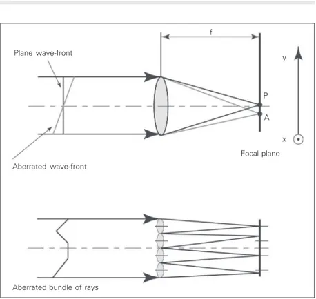
sizes and configurations for HS sensors (26). Our “home-made” HS sensor is composed of a grid of 15 x 15 micro-lenses. At the focal plane of the micro-lens array there is a high sensitivity monochromatic CCD. We explain the HS principle in the diagram in Figure 5. For a plane wave-front the focusing position on the CCD plane is exactly at the intersec-tion of the axis of the micro-lens with the CCD plane; on the other hand, for an aberrated wave-front, light focuses on a slightly shifted spot. For a set of micro-lenses the same principle applies and we will have uniformly spaced spots for a plane wave and non-uniformly distributed points for aberrated waves. The amount of dis-placement of the spots permits us to deter-mine the exact amount of wave-front aberra-tion. We will present the mathematical pro-cedures in the “Calculating optical aberra-tions from Zernike polynomials” subsection. In Figure 6 we present an example of an HS image obtained for an artificial eye cali-brated with zero dioptric power (no aberra-tions).

Image processing

In order to calculate the wave-front aber-ration, we must extract the information on the Cartesian positions of each spot from the digitized images using image processing tech-niques (12,13). The image processing of the HS patterns is the first step towards the quantification of aberration. We start by digi-tizing the HS image in Windows bitmap 8 bit format with an IBM compatible computer with a Pentium III 800 MHz Intel processor. This is accomplished with an attached frame-grabber (model Meteor, Matrox Electronic Systems, St. Regis Dorval, Quebec, Canada). The goal is to find the “center of mass” of each spot. We start by analyzing the distribu-tion of gray levels for horizontal and vertical lines along the image. From this distribution we determine a set of grids in such a way that each cell contains a spot. From the gray level

Figure 5. Principle of the Hartmann-Shack (HS) sensor. Upper diagram, A plane wave-front hits a single micro-lens and focuses at a point P located over the optical axis and at a distance f from the lens; for the same micro-lens an aberrated wave-front focuses at point

A, also on the focal plane but shifted away from the optical axis. Lower diagram, For a set of micro-lenses, an aberrated wave-front will focus on unevenly spaced points (shifted away from the optical axis of each micro-lens) over the focal plane. It is the quantification of the individual shifts that allows one to determine the local slopes of the wave-front and then, from this information, retrieve the entire wave-front surface. The x,y arrows to the right of the upper diagram show the coordinate system directions (y is pointing upwards and x is coming outside from the page) used according to Equations 7 and 8.

Figure 6. Hartmann-Shack image obtained with our instrument for an artificial mechanical eye cali-brated with no aberration (zero diopter), i.e., emmetropic. Plane wave-front

Aberrated wave-front

Focal plane P

A y

x

Aberrated bundle of rays

distribution inside each cell we determine the centroid of the spot by using equations:

,

, 1

,

, 1

( , ) ( , )

( , ) M N

m n

spot _{M N}

m n

x m n g m n x

g m n

¤

¤

,

, 1

,

, 1

( , ) ( , )

( , ) M N

m n

spot _{M N}

m n

y m n g m n y

g m n

¤

¤

where m and n are the horizontal and vertical pixels inside the considered cell,

x and y are the horizontal and vertical positions of the pixel in mn, and g is the intensity of gray level in an 8-bit gray scale image (0 means totally black and 255 means totally white).

Column A in Figure 7 shows the results of image processing for all calibrated aberra-tions, with centroids marked with a cross. As stated before, from the difference in centroid position for a plane wave and an aberrated wave, it is possible to calculate the front aberration (commonly called the wave-front function and represented by W) using special polynomials called Zernike polyno-mials (27) and mean square interpolation. We will now describe the mathematical pro-cedures used for this purpose.

Calculating optical aberrations from Zernike polynomials

Although Seidel polynomials are exten-sively used in the description of optical aber-rations they have certain limitations that are not present in Zernike polynomials (see a list of the first 15 Zernike polynomials in Table 1). The five conventional Seidel aberrations are classified as spherical aberration, coma, astigmatism, curvature of field (or focus shift), and distortion (or tilt). If we look carefully at Table 1, we may see that terms 13, 8 and 9, 4 and 6, 5, 2 and 3, correspond, respectively, to the Seidel aberrations. So this is the first advantage: the Seidel

aberra-tions are contained in the Zernike polynomi-als; another advantage is that the Zernike polynomials form a complete and normal-ized set of functions over the unit circle (x2

+

y2 _{£1) and also have certain properties of} invariance which are desirable in terms of symmetry and mathematical elegance, i.e., simplicity. Since a thorough and detailed discussion of Zernike polynomials and its properties is not within the scope of this article, we address the reader to what is, to our knowledge, one of the most complete discussions on the subject: appendix VII of Ref. 27, pages 905-910. We next describe some basic aspects of these polynomials. Zernike polynomials are a set of maps in the

z-axis with domain at the unit disc x2 + y2

£1 of the x,y-plane, which have the desirable property that their combinations can be found to fit well the surface shapes of reasonably “well-behaved” (28) wave-front aberrations. In polar coordinates, Zernike polynomials are the product of a radial polynomial and an azimuthal map:

\

^

( ) sin if 0

( , ) = R_{R l}l _ll

n

ZJ S R S_{S R}R _{r (Equation 3)}

where l may be any integer number and n

may be any positive integer and zero. When

l is greater than or equal to zero, the sine function is used and when it is smaller than zero the cosine function is used. The radial components of the Zernike polynomials are given by:

(n- )/2

-2 0

(-1) ( - )! ( )

![( + )/2- ]![( - )/2- ]!

¤

s n

n s R

s n m s n m s J

J _{S S}

(Equation 4)

The Zernike polynomials are thus a set of orthogonal maps defined in the unit circle. Their orthogonallity condition is expressed by:

1

´ ´ 0 0

´ ´ 2

( ) ( ,

2( +1)

, )

° °

Q _{S R SR S S R} Q _{E E}

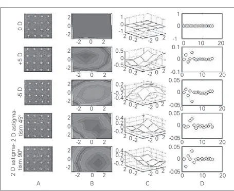
Figure 7. Results for all five measurements. A, Hartmann-Shack (HS) images for all five aberrations showing HS spots with superimposed “centers of mass” (gray crosses) detected by our image process-ing algorithm. B, Two-dimensional view of the wave-fronts calculated from the Zernike coefficients retrieved from the HS spots in A and from Equations 6-13. C, Same as in B, but plotted as three-dimensional (x, y, z) graphs. D, Zernike coefficient values for each aberra-tion. Notice that for the plane wave-front they are all zeros, as expected. These are the Zernike coefficients which are added to Equation 9 in order to retrieve the wave-fronts plotted in B and C.

0 D

+5 D

-5 D

2 D astigma- tism 45

º

2 D astigma- tism 90

º

2 0 -2

2 0 -2

2 0 -2

2 0 -2

2 0 -2

1 0 -1

0.5 0 -0.5

0.2 0 -0.4 -0.2

0.4 0.2 -0.20

0.4 0.2 -0.20 -2 0 2

-2 0 2

-2 0 2

-2 0 2

-2 0 2

A B C D

1

0

-1 0.1

0

-0.1 0.05

0

-0.05 0.05

0

-0.05 0.05

0

-0.05

0 10 20

0 10 20

0 10 20

0 10 20

0 10 20

2 0_-2

2 0_-2

2 0_-2

2 0_-2

2 0_-2

2 0 -2

2 0 -2

2 0 -2

2 0 -2

2 0 -2

Table 1. Set of the first 15 Zernike polynomials.

Term Polar Cartesian Meaning

Z1 (x, y) 1 1 Constant term

Z2 (x, y) r sin q x Tilt in x direction

Z3 (x, y) rcos q y Tilt in y direction

Z4 (x, y) r2 sin(2q) 2xy Astigmatism with axis at ±45º Z5 (x, y) 2r2 - 1 -1 + 2y2 + 2x2 Focus shift

Z6 (x, y) r2 cos(2q) y2 - x2 Astigmatism with axis at 0 or 90º Z7 (x, y) r3 sin(3q) 3xy2 - x3

Z8 (x, y) (3r3 -2r) sin q 2x + 3xy2 + 3x3 Third order coma along x axis

Z9 (x, y) (3r3 -2r) cos q -2y + 3x2y + 3y3 Third order coma along y axis

Z10 (x, y) r3 cos(3q) y3 -3x2y

Z11 (x, y) r4 sin(4q) 4y3x -4x3y

Z12 (x, y) (4r4 -3r2) sin(2q) -6xy + 8y3x + 8x3y

Z13 (x, y) 6r4 -6r2 + 1 1 -6y2 -6x2 + 6y4 + 12x2y2 + 6x4 Third order spherical aberration

Z14 (x, y) (4r4 -3r2) cos(2q) -3y2 + 3x2 + 4y4 -4x2y2 -4x4

where d is the Kronecker Delta, i.e.,

\

^

x

p p

pp p p

E ’

’ ’ (Equation 6)

for integer values of p.

The main motivation for using Zernike polynomials is that they describe the shapes of four conventional Seidelaberrations with high precision. Because there is no limit to the number of terms that may be used, many higher order aberrations can be described by Zernike polynomials, among them coma, 3rd order spherical aberration, etc. The choice of exactly how many terms to use has been discussed at a specific meeting (29) of Vi-sion Scientists, and the convention adopted was to use the first 15 Zernike terms, which are shown in Table 1. Actually, this choice is based on the fact that it is enough to use the first 15 linearly independent Zernike poly-nomials in order to obtain a highly accurate description of the most common aberrations found in human eyes (29). These polynomi-als, in mathematical terms, comprise a set of linearly independent polynomials in two indeterminates with a degree of 4 or less, which are orthonormal with respect to the inner product given in Equation 5.

We mention in the section “Optical con-figuration” the possibility of calculating the wave-front aberration from the wave-front slopes. Based on Figure 5, we may write the slopes in the x and y directions as:

a c x

x x W

f ’

(Equation 7)

a c y

y y W

f ’

(Equation 8)

where (xa, ya) is the coordinate of a spot from

an aberrated wave-front, (xc, yc) is the

coor-dinate of the reference spot, i.e., a non-aberrated, plane wave-front, and f is the fo-cal length of the micro-lenses. If we use a single index k as a function of n and l (the

indexes of Equations 3-5), namely,

( 1)

1

2 2

n n n l

k (Equation 9)

then we may write the wave-front as:

15

1

( , )

( , )

k

W x y

C Z

x y

=

=

∑

and its partial derivatives as

15 ’

1

( , )

( , ) k

x k

k

dZ x y

W x y C

dx

=

=

_∑

15 ’

1

( , )

( , ) k

y k

k

dZ x y

W x y C

dy

=

=

∑

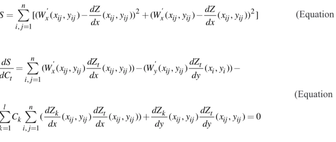
Note that k is the number of the Zernike term according to Table 1. In order to find the Zernike coefficients for a specific wave-front, we perform a minimum square fit for all i, j centroids which form the HS image. This procedure consists of minimizing the sum (see Equation 13) relative to each Zernike coefficient, and therefore we have to find dS/ dCt = 0 for t = 1, ...., k (see Equation 14) from

where we extract a square linear system AC

= b with k equations and k unknown values of C. By solving this linear system through conventional procedures (LU decomposition and Gaussian elimination method) (30) we find 15 values of C for each measured eye. For a flat wave-front the partial derivatives

dW/dx and dW/dy are zero, and we therefore obtain a C = 0 solution, which by the general equation (10) yields W(xij, yij) = 0, a plane

others. In contrast, if there is a greater amount of astigmatism at 45º, the fourth term will predominate. In the next section we show results for several calibrated aberrations on an artificial eye.

Results

Measurements were made on a mechan-ical (artificial) eye which was calibrated with five different types of ametropia: zero diop-tric (D) power, i.e., emmetropic (0 D), hy-peropic (+5 D), myopic (-5 D), and 2 D astigmatism with axis at 45º and 90º. Image processing was accomplished separately for each aberration (see Figure 7, column 1) and results were plotted in several different out-puts.

In Figure 7, from the left to the right column, we may see results for the image processing, two-dimensional color-coded maps for the wave-front, surface maps and, finally, the Zernike coefficients for each of the 15 terms in Table 1. A qualitative analy-sis of the first row (0 D) shows regularly spaced dots, a color map with one color, a plane of height zero, and coefficients all with a zero value. This is obviously in accor-dance with the expected values for a zero dioptric eye, i.e., with no aberrations, there-fore resulting in a plane wave leaving the eye.

The same qualitative analysis for the other

eyes shows the validity of the results. For example, in the cases of +5 D and -5 D, we know that the wave-front should look like a dome-shaped surface, facing downwards for the myopic and upwards for the hyperopic eye. This is in agreement with the expected shapes of wave-fronts leaving eyes with dif-ferent low order aberrations (Figure 8).

It is possible to relate the wave-front measurements to those of autorefractors.

Figure 8. Differently shaped wave-fronts leaving three types of eye: myopic, hyperopic, and emmetropic. This is simply an al-ternate view of these common eye aberrations, which are usu-ally explained by drawing paraxial rays from outside to inside the eye. Here we do the contrary: a point light source directed at the retina generates a spherical wave-front which leaves the eye. Because the emmetropic eye is a “perfect” optical system its re-fractive power is such that a spherical wave-front leaves the eye paraxially, i.e., in the form of a plane wave. The myopic eye

has a “stronger” than necessary optical power so light rays leave the eye in converging rays. The opposite happens with the hyper-opic eye, which refracts light less than necessary.

Plane wave-front

Emmetropic eye

Converging wave-front

Myopic eye

Diverging wave-front

Hyperopic eye

(Equation 13)

(Equation 14)

2 2

, 1

[( ( , ) ( , )) ( ( , ) ( , )) ]

¤

dZ dZ

S W x y x y W x y x y

dx dx

’ ’

, 1

( ( , ) ( , )) ( ( , ) ( , ))

n

t t

x ij ij ij ij y ij ij i i

t i j

dZ dZ

dS

W x y x y W x y x y

dC

¤

’ ’

1 , 1

( ( , ) ( , )) ( , ) ( , ) 0

l n

k t k t

k ij ij ij ij ij ij ij ij

k i j

dZ dZ dZ dZ

C x y x y x y x y

dx dx dy dy

Regardless of the typical high resolution data of HS, it is still possible to retrieve conventional dioptric power values for the best spherocylinder lens that describes the eye’s lower order aberrations. If we consider the spherocylindrical lens as

Wlens = 2C4xy + 2C5(x2 + y2) + C6(y2 - x2) (Equation 15)

the sphere (fD), cylinder (fA) and axis (a)

may be written as:

2 2 4 6

2 4 6 a a

A

r

G (Equation 16)

6 6 4 4

6 6

4 4

90 arctan( ) 0

arctan( ) 0

C C

for

C C

C C

for

C C

B

« º

® ®

® ®

® ®

® ®

® ®

® ®

¬_® »_®

® _b ®

® ®

® ®

® ®

® ®

­ ¼

(Equation 17)

5 2 4

D

C

d

G (Equation 18)

where d is the diameter of the entrance pupil. The root mean square errors for the meas-urements shown in Figure 7 were as follows: 0.04 D for sphere and cylinder and 4º for axis. It is known that autorefractors have typically errors of 0.12 D for sphere and cylinder and 5º for axis. We may see from these preliminary measurements that the wave-front device allows for more precise examination. We believe this precision is reproducible for eyes of the general popula-tion (preliminary tests are currently being conducted in our laboratory (31)).

Discussion

We have demonstrated the precision of the HS wave-front sensor in measuring opti-cal aberrations of an artificial opti-calibrated eye. Tests on real eyes should be conducted to verify and validate the technique.

One common difficulty of instruments

when attempts at measuring refractive errors are made occurs during accommodation. It is not always possible to repeat the measure-ments with the crystalline lens at exactly the same dioptric power. This certainly makes the reproducibility of these instruments much lower than expected. Our intention here was not to compare the precision of the whole refractive instrumentation and therefore we did not consider accommodation (our artifi-cial eyes do not have a lens). Our intention was to provide insight about how promising the wave-front technique may be when com-pared to conventional autorefractors in terms of resolution and precision. An accommo-dating system, when well functioning, may be applied to either type of instrument, per-mitting absolute precision comparisons for daily measurements in the human popula-tion. We are currently building a genuine accommodation device using a micro-con-trolled moveable optical system, which is electronically controlled by a software through the parallel port interface of an IBM-compatible PC. The principle of this accom-modation system is based on the optical diagram shown in Figure 3 (32).

that computerized corneal topography re-placed the traditional keratometer and the photokeratoscope. Moreover, the wave-front will permit precise corneal ablations, resulting in algorithms that may execute what is being called “customized corneal ablations” (34).

References

1. Liang J, Grimm B, Goelz S & Bille JF (1994). Objective measurement of wave aberrations of the human eye with the use of a Hartmann-Shack wave-front sen-sor. Journal of the Optical Society of

America, 11: 1949-1957.

2. Thibos LN (2000). Principles of Hartmann-Shack aberrometry. Journal of Refractive

Surgery, 16: 540-545.

3. Scheiner C (1619). Oculus, sive funda-mentum opticum. Innspruk, Austria. 4. Tscherning M (1894). Die

monochro-matischen Aberrationen des mensch-lichen Auges. Zur Physiologischen Psy-chologie der Sinnesorgane, 6: 456-471. 5. Howland B (1960). Use of crossed

cylin-der lens in photographic lens evaluation.

Applied Optics, 7: 1587-1588.

6. Campbell FW & Robson JG (1959). High speed infrared optometer. Journal of the Optical Society of America, 49: 268-272. 7. Charman WN & Heron G (1975). A simple

infra-red optometer for accommodation studies. British Journal of Physiological Optics, 30: 1-12.

8. Cornsweet TN & Crane HD (1976). Servo-controlled infrared optometer. Journal of the Optical Society of America, 60: 548-554.

9. Shikawa YY (1988). Eye refractive power measuring apparatus. US Patent No. 4755041, July 5.

10. Plácido A (1880). Novo instrumento de exploração da córnea. Periodico d’ Oftal-mologia Pratica, 5: 27-30.

11. Oliveira MCF & Minghim R (1997). Uma introdução à visualização computacional.

XVI Jornada de Atualização em Informá-tica, Brasília, DF, Brazil, August 2-8, 85-127.

12. Gonzalez RC & Woods RE (1992). Digital Image Processing. Addison Wesley Pub-lishing Company, Reading, MA, USA. 13. Carvalho LA, Silva EP, Santos LER, Tonissi

SA, Romão AC & Castro JC (1996). Detecção de bordas de imagens refletidas pela superfície anterior da córnea. III Fórum Nacional de Ciência e Tecnologia

em Saúde, Campos de Jordão, SP, Brazil. 14. Mandell RB & St Helen R (1971). Math-ematical model of the corneal contour.

British Journal of Physiological Optics, 26: 183-197.

15. Halstead MA, Barsky BA, Klein SA & Mandell RB (1995). A spline surface algo-rithm for reconstruction of corneal topog-raphy from a videokeratographic reflec-tion pattern. Optometry and Vision Sci-ence, 72: 821-827.

16. Rabinovitz YS (1998). Keratoconus. Sur-vey of Ophthalmology, 42: 297-319. 17. Rabinovitz YS & Rasheed K (1999). KISA%

index: A quantitative videokeratography algorithm embodying minimal topo-graphic criteria for diagnosing keratoco-nus. Journal of Cataract and Refractive Surgery, 25: 1327-1335.

18. Donshik PC, Reisner DS & Luistro AE (1996). The use of computerized video-keratography as an aid in fitting rigid gas permeable contact lenses. Transactions of the American Ophthalmological Soci-ety, 94: 135-143.

19. Budak K, Khater TT, Friedman NJ, Holla-day JT & Koch DD (1999). Evaluation of relationships among refractive and topo-graphic parameters. Journal of Cataract and Refractive Surgery, 25: 814-820. 20. Carvalho Luis Alberto V, Castro JC,

Chamon W, Schor P & Carvalho Luis An-tonio V (2001). Wave-front measurements of the human eye using the Hartmann-Shack sensor and current state-of-the-art technology for excimer laser refractive surgery. Lasik and beyond Lasik. Chapter 31. In: Boyd BF(Editor), Highlights of Oph-thalmology. Pergamon Press, Oxford, England.

21. Babcock HW (1953). The possibility of compensating astronomical seeing. Publi-cations of the Astronomical Society of the Pacific, 65: 229 (Abstract).

22. Tyson RK (1997). Principles of Adaptive Optics. 2nd edn. Academic Press, San Diego, CA, USA.

23. Hartmann J (1900). Bemerkungen über

den Bau und die Justierung von Spektro-graphen. Zeitschrift für Instrumenten-kunde, 20: 47.

24. Shack RV & Platt BC (1971). Production and use of a lenticular Hartmann screen.

Journal of the Optical Society of America, 61: 656.

25. Junior FS, Yasuoka F, Santos J, Carvalho LA & Castro JC (2001). Desenvolvimento de um sistema para medidas de aberra-ções ópticas do olho humano usando a técnica de Hartmann-Shack. XXIV Encon-tro Nacional de Física da Matéria Conden-sada, Óptica (Lasers e Instrumentação Óptica), São Lourenço, MG, Brazil, May 15-19, 457.

26. Geary JM (1995). Introduction to wave-front sensors. In: O’Shea DC (Editor), Tu-torial Texts in Optical Engineering. Vol. TT 18. SPIE Press, New York, NY, USA. 27. Born M (1975). Principles of Optics.

Cam-bridge University Press, UK (ISBN: 0521642221, 7th edn., October 1999), 464-466.

28. Cournant R & Hilbert D (1953). Methods of Mathematical Physics. Vol. 1. 1st En-glish Edition. Interscience Publishers, New York, NY, USA.

29. Thibos LN, Applegate RA, Schwiegerling JT & Webb R (2000). VSIA Standards Taskforce members. Report from the VSIA taskforce on standards for reporting optical aberrations of the eye. Journal of Refractive Surgery, 16: S654-S655. 30. Press WH, Flannery BP, Teukolsky SA &

Vetterling WT (1989). Numerical Recipes in Pascal - the Art of Scientific Computing. Cambridge University Press, Cambridge, UK, 37-39.

31. Santos JB, Scannavino Jr FA, Carvalho LAV, Filho RL & Castro JCN (2001). Sen-sor Hartmann-Shack para uso oftalmoló-gico. XXIV Encontro Nacional de Física da Matéria Condensada, Óptica (Lasers e Ins-trumentação Óptica), São Lourenço, MG, Brazil, May 15-19, 457.

32. Scannavino Jr FA, Filho RL, Santos JB, Carvalho LAV & Castro JCN (2001).

Ins-Acknowledgments

trumento eletro-óptico para medidas au-tomatizadas da acomodação do olho humano (in vivo) durante medidas refra-tivas. XXIV Encontro Nacional de Física da Matéria Condensada, Óptica (Lasers e Ins-trumentação Óptica), São Lourenço, MG,

Brazil, May 15-19, 458.

33. Carvalho LA, Castro JC, Schor P & Chamon W (2000). A software simulation of Hartmann-Shack patterns for real cor-neas. International Symposium: Adaptive Optics: From Telescopes to the Human

Eye. Murcia, Spain, November 13-14. 34. Klein SA (1998). Optimal corneal ablation