UNIVERSITE CATHOLIQUE DE LOUVAIN
LOUVAIN SCHOOL OF MANAGEMENT
and
NOVA SCHOOL OF BUSINESS AND ECONOMICS
Can the Yield Spread predict economic growth? An assessment for European countries
Supervisor at LSM: Sophie Béreau
Supervisor at Nova SBE: Paulo Manuel Marques Rodrigues
Research Master’s Thesis
Submitted by: Rubens Guimarães Togeiro de Moura With a view of getting the degrees
Master in Economics Master in Management
I would like to thank professors Paulo Rodrigues and Sophie Béreau for supervising me with
valuable comments and suggestion throughout the execution of this work. I also would like to
express my gratitude to all my “Double Degree” friends who followed me during this
extensive academic journey: Diogo, Alberto, Marius, Natalie, Sonya, Marius, Thomas,
Martynas and Monika. “Obrigado”, “Gracias”, “Danke”, “Merci”... Thank you all! Special
Contents
1- Introduction ... 1
2- Why might the Yield Spread predict economic growth? A theoretical assessment ... 3
2.1 Explanations based on the stance of Monetary Policy ... 3
2.2 - Explanations based on consumers’ intertemporal choice ... 5
3- Data description ... 6
4- Empirical estimation ... 7
4.1) Unit root tests ... 8
4.2) In-sample estimation ... 10
4.2.1) An assessment of the Yield Spread of the full sample ... 10
4.2.2) The impact of the Global Financial Crisis of 2008 ... 16
4.2.3) Comparison with other benchmarks ... 21
4.2.4) Diebold-Mariano test ... 26
4.2.5) In-Sample: The best fit that the YS models can achieve ... 28
4.3) Out-of-sample estimation ... 29
4.3.1) Out-of-Sample: The best fit that the YS models can achieve ... 34
5- Concluding Remarks ... 35
References ... 37
Appendix A – General features ... 40
Appendix B – In-Sample analysis ... 42
Appendix C – In-Sample analysis: Benchmarks ... 46
Appendix C.1- AR model ... 46
Appendix C.2- RW model ... 48
Appendix C.3- AR + YS model ... 50
1- Introduction
Reliable forecasts of future course of economic activity are crucial inputs in the decision
making process of several economic agents. Firms, for instance, adjust their level of
production and hiring policy accordingly by knowing whether the forthcoming state of the
economy is more prone to be recessionary or expansionary. Likewise, Central Banks use this
sort of information to decide on the stances of current and future monetary policy. For hedge
funds, economic growth predictions contribute with a better design of investment strategies
for their customers.
One possible method for constructing forecasting of economic growth is through financial
variables. The usefulness of these technique lies on the possibility of building models of easy
implementation by means of data that are usually reliable and readily available (Bonser-Neal
and Morley, 1997, p.37). It was based on these sorts of data that Stock and Watson (1989)
proposed a very straightforward and successful methodology for prediction future output: the
so called yield spread (YS, hereafter), i.e., the differential of the long and short term interest
rates. The authors found that the presence of the YS was able to contribute significantly to
anticipate the future behavior of the United States’ economy. Specifically, it was observed that the higher the gap in the interest rates (i.e. the grater the yield spread), the more intense
the forthcoming economic growth was expected to be.
As of Stock and Watson’s (1989) contribution, the relationship between economic growth and the Yield Spread (YS, hereafter) was extensively investigated in the literature, being the
United States (US) the economy mostly studied. By way of illustration, Haubrich and
Dombrosky (1996) showed that a model containing the YS as the single regressors was able
to outperform, on average, others forecasts based, for instance, on the index of leading
economic indicators and a combination of lagged output and YS terms. It is also documented
in the literature cases in which the inclusion of the YS enhances the predictive content of
alternative specifications containing variables such as 3-month T-bills (Dotsey, 1997), real
FED Fund (Estrella and Hardouvelis, 1991), past economic activities (Dotsey, 1997 and
Estrella and Hardouvelis, 1991) and a combination of past inflation and index of leading
The existing studies for European economies1 are less numerous and less successful in
confirming the predictive power of the YS (see e.g. Wheelock and Wohar, 2009). In a similar
fashion as Dotsey (1997), Sedillot (2001), for Germany and France, and (Berk and van
Bergeijk, 2000), for a set of 10 countries of the Euro Zone, concluded that it was very reduced
the positive marginal contribution brought by the YS (or its lagged version in Berk and van
Bergeijk, 2000) to output autoregressive models.
Motivated by the absence of an expressive quantity of publications dedicated to European
economies, this study aims at contributing with the existing literature through both cross and
within-country analysis, proposing a fully revision about the capability of the YS to act as a
reliable leading indicator in the last three decades.
It is not our objective here find out the sort of estimation method that generates the most
accurate forecasts. Rather, grounded in previous publications (as per in Berk and van
Bergeijk, 2000, Sedillot, 2001, Hamilton and Kim, 2002, Bonser-Neal and Morley, 1997,
among others), we are going to test the strength of the relationship between YS and economic
growth when this is treated as linear. To this end, it will be thoroughly investigated whether
the predictive content of the YS is sensitive to (i) changes in forecast horizons; (ii) the matter
as economic activity is measured; (iii) drastic macroeconomic downturn, namely the Global
Financial Crisis which started in 2008 and (iv) different forecasting techniques. Ultimately, it
is intended to provide complementary insights to the analysis of Berk and van Bergeijk (2000)
and Sedillot (2001). In particular, we will verify whether the lack of predictive power of the
YS in presence of past economic activity can be extended for a different set of countries and
for a sample period posterior to the implementation of the monetary union.
Besides this introduction, this study is structured in four more sections. Section 2 reviews
some of the theoretical arguments for justifying the relationship between economic growth
and the differential of long and short interest rates. Afterwards, the validity of the same
relation will be empirically tested and thoroughly analyzed in the next two sections. Lastly,
section 5 summarizes the main empirical findings obtained in the previous parts.
1
2- Why might the Yield Spread predict economic growth? A theoretical assessment
One can find in the current literature mainly two different underlying causes for explaining
the positive relationship between yield spread and future economic activity. One has its roots
in the path of monetary policy adopted by Central Banks, and the other focuses on consumers’ investment decisions over time. In what follows, we will briefly describe some of the general
features of each theory.
2.1 Explanations based on the stance of Monetary Policy
There are different theories which resort to monetary policy arguments to advocate in favor of
a legitimate YS-economic growth relationship. In what follows, we will shed some lights on
the most disseminated theories in the literature.
a) Expectations hypothesis: This theory prescribes that one can build a yield curve based
on the following equation:
∑
[ ]
where stands for the yields of a n-period zero-coupon bond, θt is the risk premium in
period t and E[.] the expectations operator.
In addition to a risk-premium, we can also observe that the long-term rates can be computed
as a weighted average of expected future short-term rates. The rationale of this theory lies in
the premise that investors may not expect to acquire different returns by investing in bonds of
different maturities - otherwise they would be able to realize arbitrage gains. Moreover, the
uncertainty associated with the path of future short-term interest rates makes investors
demand a risk premium for holding bonds of higher maturities. In these circumstances, as the
long-term interest rates would tend to become larger than short-term rates, one may find a
reason to justify a positive slope of the yield curve.
Given the arguments in favor of a positive slope of the yield curve, one may be interested in
thinking about: (i) the possible causes that make the slope of the yield curve negative and (ii)
the relationship between this reversion and the future occurrence of economic slowdown
periods.
According to Passaro (2007), changes in interest rates' risk premium are thought to be
insignificant, at least in the short-run. In this manner, the source of change in the signal of the
yield spread should be attributed to fluctuations in the future short-term interest rates. In
particular, the expectation that a recessionary period is approaching leads investors to believe
that Central Banks will decrease future interest rates in order to stimulate and sustain the level
of output. Therefore, the belief that an expected deterioration in future economic activity will
follow, flattens – and eventually inverts - the slope of the yield curve.
b) Counter cyclicality of Monetary Policy: Central Banks are able to speed up or slow
down the rate of economic growth of a particular country by performing changes in the level
of interest rates.
As a manner of promoting a faster economic growth in the short-run, Central Banks may
adopt an increase in money supply, which will result in a reduction of both long and short
term interest rates. The impact of these reductions, however, is not identical. As stated by
Estrella, Rodrigues and Schich (2000), a loose monetary policy leads to a greater decline in
the short-term interest rate. The argument for that is that a reduction in the short-term interest
rate may generate a higher inflation rate and, as a manner to counterbalance the increase in the
price level, Central Banks may wish to increase forthcoming interest rates. Therefore, one
may realize a positive relationship between the slope of yield spread and future economic
output.
By the same token, one may expect an analogous outcome for the case when Central Banks
opt for a tighter monetary policy. Shrinkage in money supply may lead to a less steep yield
curve – as one may expect a more intense increase in the short term interest rate than in those of longer maturities - followed by a slower rate of economic growth.
c) The importance assigned by policymakers to future inflation: following a procedure
centered less on a “heuristic” and more on an “explicit model” basis (Estrella, 2005, p. 3), Estrella, (2005) and Estrella (1997) demonstrate analytically the pertinence between a positive
tools: a Phillips curve, a dynamic IS curve, the Fisher equation, the expectations hypothesis
and the monetary policy rule of which the Taylor Rule is an example (Estrella, Rodrigues and
Schich, 2000, p.7).
The conclusions that can be found in Estrella (1997) are that the predictive power of the yield
curve is partially related with the preferences that policymakers have over the deviation of
both output and inflation from their target (Duarte, Venetis and Payá, 2004). In particular, this
relationship is especially robust when the monetary policy is exclusively focused on the
promotion of output growth, whereas the correlation becomes weaker when Central Banks
target to combat inflation only. Estrella (2005) adds to these results that the yield curve, as a
leading indicator, performs (i) greatly when monetary authorities are more concerned with
changes in the interest rate, alternatively to its levels and (ii) rather poorly, when Central
Banks’ reactions to both inflation and output deviations approaches infinity.
2.2 - Explanations based on consumers’ intertemporal choice
The origin of this approach is supported by the works of Harvey (1988)2 and Hu (1993)2
.
Resorting to microeconomic foundations, the authors develop models for determining the
consumers’ optimal level of consumption over time.
A core assumption of these models is that consumers are better off by having a stable income
stream regardless of the stage of the Business Cycle than the situation in which they
experience high levels of income during expansionary periods and low income during
downturns. In this sense, in a world where the only financial asset available to be invested is a
default-free bond, consumers would prefer to hold long term bonds when they expect a future
period of recession. By acting in this manner, one will observe an increase in the demand for
these bonds, leading to an increase in their prices and, hence, a reduction in their yield.
Moreover, consumers may wish to fund the acquisition of the long-term bonds by selling
bonds of shorter maturities. This behavior would result in an increase in the yield of
short-term bonds.
2
Given the theoretical arguments to support the positive relationship between the YS and
economic growth, it is relevant to assess their empirical validity. The next sections aim to
provide an in-depth investigation of the strength of this relationship in a sample of 12
European countries.
3- Data description
We tested the quality of the YS as a leading indicator the following countries: Belgium,
France, Germany, Ireland, Italy, Netherlands, Norway, Portugal, Spain, Switzerland, Sweden
and the United Kingdom. The criteria chosen in the selection of these countries was based on
the availability of data. In particular, European economies were chosen for which we could
find quarterly data starting from the beginning or the middle of the decade of 1980 (a more
precise description is presented in the appendix A). For all countries considered the last data
available is the last quarter of 2013.
Regarding the constructions of the variables of interest, the yield spread was computed in
consonance with the procedure widely used in the literature. In particular, Moneta (2003) has
found that the spread that results from the 10-years minus 3-months rates outperforms any
other spread, when one is interested in comparing different forecasts. In this manner, for each
country of the sample, the yield spread was computed as:
where the corresponds to the yield on government bonds with a maturity of ten years and
to the 3-month money market rates3. Both series were extracted from Eurostat. A
historical series from each country can be found in the appendix A.
Concerning the measurement of economic activity, two indicators were adopted: Real Gross
Domestic Product (real GDP, hereafter) and Industrial Production (IP, hereafter). Both series
3
It is common practice in the literature which analyzes the case of the US to treat the short term interest rate as the 3-months T-bills interest rates. For the countries of the European Union, after the implementation of the Euro as common currency created a lack of a specific short term government bond for every country which joined the monetary union. In these circumstances, one has decided to replace this rate for the one which is the most representative rate according to the Eurostat: the interbank 3-month money market rate.
were collected on a quarterly basis from the OECD’s database. The real GDP series used was the one which accounts for the volume estimates, based on fixed PPPs, with seasonally
adjustment (expenditure approach), whereas the IP refers to the Production and Sales index
(MEI).
In order to obtain the average annualized growth of future economic activity (represented by
the variable g) over the next k quarters, one has computed:
where k was estimated from 1 to 8 quarters ahead and Y denotes both real GDP and IP for
each country.
It is relevant to highlight that all data used in this analysis is revised data and not real time
based. The reason for this choice lies in the fact that one aims at investigating the “true” realization of economic growth rather than their expected, preliminary values.
4- Empirical estimation
Having collected data of interest rates and future economic activity, we may test the
predictive power of the yield spread over the economic growth. The analysis will be
performed in two stages, and through two different forecasting techniques. In a first moment,
one adopts an in-sample procedure, which consists in estimating an average relationship of
explanatory variables over the dependent variable, taking into account the whole sample
period. In this sense, one estimates a single coefficient for the whole sample period, despite of
the fact that some information was not available for market participants in the moment that
the forecasting was carried out (Bonser-Neal and Morley, 1997, p.41). The second technique
explored is the so called out-of-sample. Under this framework, one performs the forecasting
based exclusively on the existing information to market participants at some moment in time.
In particular, one re-estimates the parameters of the model as new information becomes
available.
The estimation of the models of interest, for both forecasting techniques, was made through
Ordinary Least Squares (OLS, hereafter). According to Moneta (2003), an issue related with
this procedure lies in the fact that overlapping forecast horizons may generate autocorrelation
in the error terms, making the standard errors no longer valid. To correct for this drawback,
we performed an OLS estimation with Newey and West (1987) standard errors.
In the next following sub-sections, a separate analysis about the performance of both
forecasting techniques will be conducted for (i) the whole period for which one has data
available (from early 1980 to 2013) and (ii) the period that ends with the Global financial
Crisis of 2008 (which was set as the last quarter of 2008, period that was marked by Lehman
Brother’s bankruptcy). In order to fully test the predictive power of the yield spread, one will confront the quality of their forecasts with some of the benchmarks widely used in the
literature.
Before initializing the complete analysis of the aspects mentioned previously, we tested
whether the Yield Spread series satisfy the conditions of stationarity.
4.1) Unit root tests
Examining stationarity is crucial when dealing with time series data. An inappropriate
treatment of non-stationary may generate the problem of spurious regressions. A potential
source of this issue, as documented by Bueno (2008), is related with the realization of
regressions in which the series present different orders of integration.
Bearing in mind the existence of this trouble, one has opted to investigate the possibility of
unit roots in YS series through the traditional Dickey-Fuller test (DF, hereafter). In this
manner, we proceeded by conducting a test in which the underlying model includes a time
trend and constant. The null hypothesis is the existence of a unit root, while states that
the series is stationary. We also tested for a unit root in the first difference of the series based
on a test regression which included a constant term only. The rejection of the null hypotheses
The outcomes of the DF tests are shown in tables DF.1 and DF.2 for the full- sample and for
the periods prior to 2008, respectively. Based on the critical values of the DF distribution, we
indicate in red the entries which reveal indication that the series are not stationary.
Table DF.1 - Unit root test for YS series: Dickey Fuller statistics - Whole period 4
Table DF.2 - Unit root test for YS series: Dickey Fuller statistics – Prior to 20084 4 por encima de
4
The test was performed to a level of significance equal to 10%, in which the critical values of the distribution are the following:
a) Trend + intercept: -3,15 b) Intercept: -2,58
DF statistic p-value DF statistic p-value DF statistic p-value DF statistic p-value Trend + Intercept -4,45 0,003 -3,524 0,003 -3,68 0,027 -3,925 0,015
Intercept -4,16 0,001 -3,344 0,015 -3,72 0,005 -2,985 0,040
DF statistic p-value DF statistic p-value DF statistic p-value DF statistic p-value Trend + Intercept -4,075 0,009 -3,42 0,054 -3,863 0,017 -2,31 0,426
Intercept -1,937 0,314 -3,28 0,018 -3,634 0,007 -1,88 0,340
DF statistic p-value DF statistic p-value DF statistic p-value DF statistic p-value Trend + Intercept -4,49 0,002 -3,764 0,022 -3,45 0,049 -3,482 0,046
Intercept -3,36 0,014 -3,509 0,010 -2,23 0,196 -2,877 0,051
Switzerland UK
Germany Ireland
Italy Netherlands Norway Portugal
Belgium France
Spain Sweden
DF statistic p-value DF statistic p-value DF statistic p-value DF statistic p-value Trend + Intercept -3,88 0,02 -3,016 0,003 -2,90 0,165 -3,959 0,014
Intercept -4,05 0,00 -3,224 0,021 -3,04 0,034 -3,758 0,005
DF statistic p-value DF statistic p-value DF statistic p-value DF statistic p-value Trend + Intercept -3,111 0,109 -2,47 0,341- 2,82 0,193 -3,38 0,061 Intercept -2,859 0,053 -2,52 0,113 -2,820 0,059 -3,40 0,013
DF statistic p-value DF statistic p-value DF statistic p-value DF statistic p-value Trend + Intercept -4,59 0,002 -2,623 0,272 -2,42 0,37 -2,981 0,143
Intercept -4,32 0,001 -2,582 0,101 -2,08 0,25 -2,874 0,052
Belgium France Germany Ireland
Italy Nethelands Norway Portugal
As one can observe directly from the previous tables, some series are non-stationary5. Due to
that, the estimation of regressions containing these series will deserve a special treatment,
which will be further explained in the next section.
4.2) In-sample estimation
4.2.1) An assessment of the Yield Spread of the full sample
The in-sample procedure consisted in the distinct estimation of regressions, by country and by
different forecasting time horizons. In particular, for each economy that has shown to be
stationary, the following equation – which will be named YS model hereafter - was estimated:
YS model:
and for those in which unit roots were diagnosed, the first difference of the YS was used:
Recall that the forecasting period ranged from one to eight quarters ahead, i.e, k =1,2 ..., 8.
The criteria set for this choice is aligned with Hamilton and Kim (2002) and Sedillot (2001),
which portray that the predictive power of the slope of the yield curve over economic growth
lasts up to two years. Provided the fact that the dependent variable is measured as the growth
rate of both industrial production and real GDP, the “YS-IP model” will be used to allude to
the former set of regressions, whereas “YS-GDP model” will be implemented for the latter one.
Before proper examining the predictive power of YS model, one may be interested in
quantifying the expected impact that changes in the yield spread may entail over future
economic activity. Tables B.1 and B.2 (see appendix B) show that, apart from some rare
exceptions, an increase (decrease) of 1% in Yield Spread – or the first difference of that, for the countries in which the YS is not a stationary series - impacts positively (negatively) less
5
Even though Italy in the series which includes the period prior to 2008 has shown a DF statistic slightly below the critical value of interest, one has decided to include it in the group of stationary countries.
(4.1)
than 1% on the future productive path of a particular economy. This outcome is consistent
with the estimations found by Haubrich and Dombrosky (1996) and Ang, Piazzesi and Wei
(2006)6 for the US and Bonser-Neal and Morley (1997) for a set of industrialized countries.
The exact estimated values for the slope coefficients ( and their respective standard errors
can be found in respective appendix section.
As a manner of quality assessment of the YS models, we decided to resort to the use of the
R-squared and the Mean Absolute Deviation (MAD, hereafter). The choice for both tools, rather
than just one of them lies in the fact that they provide different information about the
forecasting properties of the model. The R-Squared can be interpreted as a measure of
correlation between the predicted and the actually realized values. In other words, it assesses
how variations in the dependent variable are explained by variation in the covariates. The
MAD, in turn, provides an average measure of the lack of precision of predicted values.
For the full sample, the estimated outcomes are presented in tables IS.1 through IS.2 for the
R-Squared, and in tables IS.3 through IS.4 for the MAD. Throughout, the lines in orange will
correspond to the cases in which one has measured the YS as its first difference.
The values of the R-Squared for each time forecasting horizon were computed by the
following formula:
∑ ∑ ̂ ̅
where ̂ represents the fitted values and ̅, the sample average.
Table IS.1 – Estimated R-squared: In-sample estimation for several quarters ahead - Whole Period
Dependent variable: IP
6
The comparison made here is made with the 5-years term spread, the longest one used by the authors.
Without a doubt, one observes that the most remarkable aspect refers to the poor predictive
performance of the model proposed. One can notice that the explanatory power of the yield
spread often overcomes the barrier of 10% for most of the time horizons - value that is rather
inferior to those obtained by Haubrich and Dombrosky (1996) and Bonser-Neal and Morley
(1997) - in only 4 out of the 12 economies examined. The high level of diversity in the
outcomes is worth pointing out: while the yield spread has demonstrated to be a fair predictor
of the future industrial production for Germany (especially for horizons superior to one year),
in other countries such as Italy, Portugal, Spain and Switzerland the same measure has shown
to be a rather ineffective leading indicator. Furthermore, one may observe the increasing
predictive power of the explanatory variable over the first year; followed by a reduction in
subsequent periods.
Bearing in mind the historical perspective of more than three decades, the replacement of
Industrial Production by real GDP growth as a measure of real economic activity does not
transform the yield spread model in a satisfactory one (see table IS.2). With few exceptions,
the R-squared continues to present values of reduced significance. However, one difference
between the YS-IP and YS-GDP models can be pointed out, namely, the increased predictive
power over the second year of the horizon analyzed of the latter model.
Table IS.2 - Estimated R-squared: In-sample estimation for several quarters ahead - Whole Period
Dependent variable: Real GDP
A case by case comparison with the previous model estimated, evidences rather
heterogeneous outcomes. In comparison to the regressions in which IP growth was used as
dependent variable, the models with real GDP growth performed: (i) slightly worse for short
maturities (up to the horizon of one year) and slightly better for longer maturities (cases of
France, Netherlands); (ii) slightly better for the overall period analyzed (United Kingdom);
(iii) slightly better (Norway) or slightly worse (Belgium and Ireland) for all maturities; (iv)
likewise extremely unsatisfactory (Italy, Portugal, Spain and Switzerland) and (v) drastically
different, in a positive manner (Sweden) or in a negative one (Germany).
In addition to the R-squared, we have also estimated the MAD:
∑ | |
where is the forecasting error of period t, i.e., the difference between the value predicted by
the model and the value effectively realized. This indicator enables one to compare the
forecasting performance across countries and time horizons, regardless of the number of
observations available for each country. A summary of this indicator is presented in tables
IS.3 and IS.4.
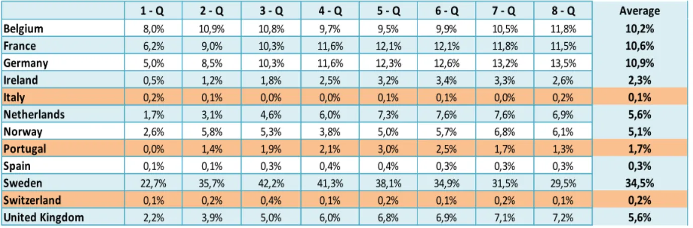
1 - Q 2 - Q 3 - Q 4 - Q 5 - Q 6 - Q 7 - Q 8 - Q Average Belgium 8,0% 10,9% 10,8% 9,7% 9,5% 9,9% 10,5% 11,8% 10,2% France 6,2% 9,0% 10,3% 11,6% 12,1% 12,1% 11,8% 11,5% 10,6% Germany 5,0% 8,5% 10,3% 11,6% 12,3% 12,6% 13,2% 13,5% 10,9% Ireland 0,5% 1,2% 1,8% 2,5% 3,2% 3,4% 3,3% 2,6% 2,3% Italy 0,2% 0,1% 0,0% 0,0% 0,1% 0,1% 0,0% 0,2% 0,1% Netherlands 1,7% 3,1% 4,6% 6,0% 7,3% 7,6% 7,6% 6,9% 5,6% Norway 2,6% 5,8% 5,3% 3,8% 5,0% 5,7% 6,8% 6,1% 5,1% Portugal 0,0% 1,4% 1,9% 2,1% 3,0% 2,5% 1,7% 1,3% 1,7% Spain 0,1% 0,1% 0,3% 0,4% 0,4% 0,3% 0,3% 0,3% 0,3% Sweden 22,7% 35,7% 42,2% 41,3% 38,1% 34,9% 31,5% 29,5% 34,5% Switzerland 0,1% 0,2% 0,4% 0,1% 0,2% 0,1% 0,2% 0,1% 0,2% United Kingdom 2,2% 3,9% 5,0% 6,0% 6,8% 6,9% 7,1% 7,2% 5,6%
Table IS. 3 – MAD: In-sample estimation for several quarters ahead - Whole Period
Dependent variable: IP
Table IS.4 – MAD: In-sample estimation for several quarters ahead - Whole Period
Dependent variable: Real GDP
The previous tables provide some interesting insights. First, the lack of accuracy exhibited by
the models is evident. On average, the framework adopted mispredicts future economic
growth in (i) more than 1 percentual point for the YS-GDP model and (ii) at least, 2.3
percentual points for the YS-IP model. Second, the choice of the dependent variable turned
out to be relevant as it alters substantially the average forecasting error and favors the
YS-GDP models. Nevertheless, switching the dependent variable does not largely modify the
comparative performance across countries. In other words, economies that demonstrated the
best outcomes in one of the models continue to behave alike in the other (e.g. France, the
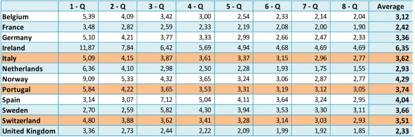
1 - Q 2 - Q 3 - Q 4 - Q 5 - Q 6 - Q 7 - Q 8 - Q Average Belgium 5,39 4,09 3,42 3,00 2,54 2,33 2,14 2,04 3,12 France 3,48 2,82 2,59 2,33 2,19 2,08 2,00 1,90 2,42 Germany 5,10 4,21 3,77 3,33 2,99 2,66 2,47 2,33 3,36 Ireland 11,87 7,84 6,42 5,69 4,94 4,68 4,69 4,69 6,35 Italy 5,09 4,15 3,87 3,61 3,37 3,15 2,96 2,77 3,62 Netherlands 6,36 4,10 2,98 2,50 2,28 1,93 1,75 1,55 2,93 Norway 9,09 5,33 4,32 3,65 3,24 3,06 2,87 2,77 4,29 Portugal 5,84 4,22 3,65 3,53 3,31 3,19 3,12 3,05 3,74 Spain 3,14 3,07 7,12 5,04 4,11 3,64 3,24 2,95 4,04 Sweden 2,70 2,59 5,82 4,30 3,94 3,53 3,30 3,11 3,66 Switzerland 4,80 3,88 3,62 3,41 3,28 3,14 3,03 2,93 3,51 United Kingdom 3,36 2,73 2,44 2,22 2,09 1,99 1,92 1,85 2,33
Netherlands and Belgium), and being the same verified for those which performed the worst
(e.g. Portugal, Ireland and Norway). Thirdly, one remarks that it is a common feature of both
YS models that the MAD decreases as the forecasting horizons increase. The only countries
which do not prove comply to this are Portugal (when real GDP is assumed as dependent
variable) and Sweden (for both cases), for all the others the lowest mean forecasting error is
observed in 8 quarters ahead.
It is also relevant to examine whether the comparative performances across countries are
sensible to the method that one uses to compute them. In other words, one may wish to know
whether, for a particular country, the selection of either the R-Squared or the MAD changes
the judgment about the predictive strength of the model. An answer to this question can be
obtained from Tables IS.5 and IS.6.
Table IS.5 – MAD: Average of YS
models – Whole Period
Table IS.6 – R-Squared: Average of
YS models – Whole Period
The value of each entry in the previous tables was computed by taking the simple average of
the respective indicator of both YS models for the period that preceded 2008. After that, we
built a ranking of performance, with countries ordered in a decreasing manner.
France 1,75
United Kingdom 1,99
Belgium 2,18
Netherlands 2,28
Germany 2,50
Sweden 2,64
Italy 2,70
Switzerland 2,72
Spain 2,86
Portugal 2,99
Norway 3,05
Ireland 5,01
Sweden 22,6%
Germany 18,9%
Belgium 13,6%
France 10,7%
United Kingdom 5,1%
Netherlands 4,9%
Norway 4,3%
Ireland 4,0%
Portugal 1,4%
Spain 0,4%
Switzerland 0,3%
From the previous tables, it is not possible to observe substantial changes in the placements of
the economies. The aspect which draws attention is the case of Ireland: the R-squared would
qualify the country as one of average comparative performance, whereas MAD suggests, by
far, the worst achievement.
One can list similarities and differences between the results provided by the estimates of the
MAD and R-squared. Regarding the common points, one may notice that overall both
indicators suggest a poor performance of the YS models (especially when the aim of the
prediction is up to 2-quarters ahead), apart from the decision of the dependent variable.
Furthermore, a comparative analysis across countries about the quality of the forecasting
preserves a similar ordination for both cases. In particular, Belgium and France have
demonstrated superior performance vis-à-vis the majority of the economies, UK is placed in
the middle of the list and other countries such as Portugal and Spain have shown to be among
the poorest fits for both YS models. A clear difference between the models lies in the time
horizon in which the forecasting becomes more effective: while the MADs favor the
predictions of 2 years-ahead, the R-squared does not provide any conclusive information
about this aspect.
4.2.2) The impact of the Global Financial Crisis of 2008
Having concluded that the historical performance of the Yield Spread as a leading indicator is
rather unsatisfactory, one may wish to observe the behavior of the indicator during less
turbulent economic periods. In order to do so, a similar analysis as in the previous section was
carried out, with the difference that the period from 2008 to 2013 was excluded from the
assessment.
Before shedding some lights on the effects of the Financial Crisis, one may wish to compare
exclusively the accomplishment of both YS models before 2008 (see tables IS.7 and IS.8).
Overall, it is clear that the adoption of real GDP as a dependent variable has a positive impact
on the fit quality of the model for countries such as France, Germany, Italy, Ireland and the
capability of the model to predict the countries’ future economic activity. Portugal and Belgium also corroborate this outcome.
Table IS.7 - Estimated R-squared: In-sample estimation for several quarters ahead – Prior to 2008
Dependent variable: Industrial Production
Table IS.8 - Estimated R-squared: In-sample estimation for several quarters ahead – Prior to 2008
Dependent variable: Real GDP
A general assessment about the influence of the Global Financial Crisis over the YS models
can be done through a comparison of the results in tables (i) IS.1 and IS.7, for the IP index
and (ii) IS.2 and IS.8 for real GDP. It is important to recall that due to the non-stationary
1 - Q 2 - Q 3 - Q 4 - Q 5 - Q 6 - Q 7 - Q 8 - Q Average Belgium 10,3% 18,4% 25,7% 28,2% 29,2% 26,8% 26,8% 27,0% 24,0% France 9,2% 11,8% 12,2% 11,9% 10,2% 7,6% 6,2% 5,8% 9,4% Germany 0,0% 0,3% 0,1% 0,2% 0,2% 0,3% 0,8% 1,2% 0,4% Ireland 1,6% 1,7% 0,7% 1,0% 0,9% 0,1% 0,0% 0,3% 0,8% Italy 0,3% 0,2% 0,1% 0,0% 0,5% 1,4% 2,7% 3,8% 1,1% Netherlands 3,6% 8,1% 3,7% 4,0% 5,4% 3,6% 4,2% 2,1% 4,3% Norway 0,0% 1,1% 1,4% 0,3% 0,0% 0,0% 0,4% 0,2% 0,4% Portugal 4,9% 10,9% 17,3% 25,8% 27,9% 29,0% 28,2% 25,9% 21,2% Spain 0,7% 0,9% 1,0% 0,5% 0,1% 0,0% 0,2% 0,5% 0,5% Sweden 2,9% 6,1% 11,1% 12,8% 12,4% 9,6% 7,9% 10,7% 9,2% Switzerland 0,0% 0,1% 0,6% 1,0% 0,7% 1,1% 1,3% 1,6% 0,8% United Kingdom 1,1% 0,2% 0,2% 0,1% 0,2% 0,3% 0,2% 0,6% 0,4%
1 - Q 2 - Q 3 - Q 4 - Q 5 - Q 6 - Q 7 - Q 8 - Q Average Belgium 13,0% 19,1% 19,8% 18,5% 18,2% 19,1% 20,5% 22,6% 18,9% France 10,4% 13,4% 14,2% 15,5% 15,2% 14,8% 14,7% 14,7% 14,1%
Germany 0,4% 0,2% 2,9% 6,1% 11,1% 12,8% 12,4% 9,6% 6,9%
Ireland 2,2% 4,8% 5,4% 4,9% 3,9% 2,6% 2,2% 2,0% 3,5%
Italy 0,0% 0,1% 0,3% 0,8% 2,5% 4,8% 7,0% 9,3% 3,1%
Netherlands 7,9% 10,7% 0,0% 0,1% 0,6% 1,0% 0,7% 1,1% 2,8%
Norway 1,3% 1,6% 1,1% 0,2% 0,2% 0,1% 0,2% 0,3% 0,6%
Portugal 4,4% 8,4% 14,2% 19,0% 21,6% 23,8% 23,2% 21,6% 17,0%
Spain 0,1% 0,0% 0,1% 0,1% 0,1% 0,1% 0,1% 0,1% 0,1%
Sweden 0,6% 0,0% 0,5% 0,3% 0,1% 0,0% 0,2% 0,0% 0,2%
Switzerland 0,2% 0,0% 0,0% 0,0% 0,4% 0,6% 0,4% 0,1% 0,2%
behavior of some series, some models were used taking the YS in its first difference, rather
than the level as was the case for other countries. As a consequence, one should relativize
simple comparisons involving the R-squared generated by different underlying models.
As a starting point, let us observe the changes in the behavior of the YS-IP models. In
comparison to the peer model which incorporates the whole sample period, one can state that,
for the majority of the countries, the crisis neither boosted the predictive power of the model
nor contribute to worse them. For the other economies, the incorporation of post-2008
changes unequivocally their performance, either for the good or for the bad.
Another outcome brought by the YS-IP models prior to 2008 confirms what was observed for
the full sample analysis: for the majority of the countries, the forecasts generated for short
time horizons proved to be more accurate than those for more quarters ahead.
The idea that the Financial Crisis had, globally speaking, a neutral effect over the predictive
quality of the models should not be extended to the YS-GDP regressions. On the one hand, it
is possible to observe the cases of Belgium, and France in which the economic downturn has
greatly penalized the models which incorporate real GDP as the dependent variable. In this
context, the Portuguese situation is especially remarkable. Prior to 2008, Portugal presented
the highest R-squared for a set of time horizons, but the emergence of the worldwide crisis led
to a complete collapse of the predictive quality. On the other hand, we can indicate examples
that go in the opposite direction: Sweden and Germany have shown to provide more powerful
explanatory power when the full sample is taken into account to perform the estimation.
As in the case of the full-sample period, one can also investigate the quality assessment of YS
models through the MAD. This indicator is presented in the following tables for the 12
countries and for the 8 time horizons of interest.
Table IS.9 – MAD: In-sample estimation for several quarters ahead – Prior to 2008
Dependent variable: IP
Table IS.10 – MAD: In-sample estimation for several quarters ahead – Prior to 2008
Dependent variable: Real GDP
Before focusing properly on the effects of the economic collapse that started in 2008, it is
interesting to notice that, alike to what was noticed in the full sample examination, the models
using real GDP as the dependent variable provide a greater average forecasting error when
compared with those which use the IP index.
If the analysis of the R-squared does not demonstrate a clear striking effect of the 2008-Crisis
over the reliability of the YS models for the sample, the same cannot be said when the
1 - Q 2 - Q 3 - Q 4 - Q 5 - Q 6 - Q 7 - Q 8 - Q Average Belgium 5,04 3,52 2,78 2,39 1,94 1,82 1,72 1,70 2,61 France 3,14 2,35 2,09 1,87 1,72 1,64 1,51 1,45 1,97 Germany 4,74 3,65 3,18 2,93 2,69 2,48 2,36 2,22 3,03 Ireland 11,53 7,42 6,23 5,61 4,76 4,58 4,52 4,53 6,15 Italy 4,68 3,59 3,10 2,81 2,57 2,36 2,14 1,95 2,90 Netherlands 5,69 3,48 2,58 2,15 1,83 1,55 1,38 1,25 2,49 Norway 8,27 4,77 3,86 3,27 2,91 2,76 2,76 2,64 3,91 Portugal 5,50 3,78 3,16 2,80 2,60 2,36 2,28 2,24 3,09 Spain 2,28 2,24 7,24 5,10 4,12 3,70 3,29 3,02 3,87 Sweden 2,65 5,74 3,71 3,13 2,66 2,34 2,17 2,04 3,05 Switzerland 4,61 3,45 3,14 2,78 2,57 2,36 2,16 1,99 2,88 United Kingdom 3,17 2,42 2,14 1,95 1,80 1,72 1,67 1,62 2,06
forecasting errors are considered. Disregarding the period after 2008 leads to a substantial
reduction in the MADs for all the countries analyzed, regardless of the manner one wishes to
measure future economic activity.7
If on the one hand, the Global crisis has contributed to ruin the predictive strength of the
model, on the other, it has presented some sign of preservation. For instance, a comparison
between each YS model with its similar for the full sample enables one to conclude that (i)
there were no significant changes in the overall relative performance across countries; (ii) the
model has demonstrated to be less erratic for the regressions that aim at predicting economic
growth for 8 quarters ahead and (iii) Ireland has shown to be by far the economy with the
poorest performance.
As in the case of the full sample analysis, one may be interested in establishing a performance
ranking based on the different assessment tools in order to compare whether they influence
countries’ relative positions. Results are shown in the tables IS.11 and IS.12.
As a general feature, it is possible to remark that, there are significant changes in the relative
position of the countries from one ranking to the other, and, these variations have shown to be
rather drastic in the cases such as Portugal, Ireland and the UK. Additionally, one observes
that, out of the 12 economies, only Belgium and France top performed in both indicators,
whereas only Spain and Norway have demonstrated to be among very low reliability of the
YS models.
7
Table IS.11 – MAD: Average of YS
models – Prior to 2008
Table IS.12 – R-Squared: Average of
YS models – Prior to 2008
The crisis also exerted significant influence over the slope coefficients, as observed in the
appendix B. As it was explained in section 2, one may expect a positive signal for the
coefficients . This theoretical prediction, however, is not empirically confirmed for a high
number of countries when the whole period of estimation is set8, even though the contrary is
commonly verified for prior-2008. Besides the inversion in the signal, one can also highlight
an ambiguous effect of the crisis over their magnitude: when the model is estimated for the
sample that includes the period after 2008, a given change in the yield spread impacts
significantly the expected future economic growth, but the sign of the variation is far from
being unanimous.
4.2.3) Comparison with other benchmarks
Presented a general assessment about the forecast quality of a model that assumes the YS as
the only explanatory variable, one may be interested in comparing these results with the
8
The signal is particularly puzzling for the case of France: regardless the dependent variable chosen and the sample period taken into account, the models has often presented a combinations of negative coefficients and a rather high t-statistics, which is an argument to in favor of the significance of the coefficient.
France 1,46
United Kingdom 1,70
Belgium 1,86
Netherlands 1,88
Italy 2,08
Switzerland 2,15
Germany 2,31
Sweden 2,33
Portugal 2,48
Spain 2,70
Norway 2,80
Ireland 4,56
Belgium 21,4%
Portugal 19,1%
France 11,7%
Sweden 4,7%
Germany 3,7%
Netherlands 3,6%
Ireland 2,1%
Italy 2,1%
United Kingdom 1,7%
Norway 0,5%
Switzerland 0,5%
performance of alternative models. To be consistent with the choice widely disseminated in
the literature, we are adopting the following benchmarks: a pure autoregressive models (AR,
hereafter), a autoregressive combined with the yield spread (AR + YS, hereafter) and a
Random Walk model (RW, hereafter). The order of the AR was chosen to be equal to 1 for
both cases. In particular, the outcomes of interest will be derived from the following
regressions:
AR Model
RW Model
AR + YS Model
The model 4 was estimated in first difference for the cases in which the YS has demonstrated
evidences of non-stationarity.
In this section, our objectives are twofold. Firstly, as per se in Haubrich and Dombrosky
(1996) and Bonser-Neal and Morley, 1997), it is of our interested to observe how powerful
the YS model can be in comparison to the others. Secondly, following Berk and Bergeijk
(2000) and Sedillot (2001), we intend to assess whether the YS can contribute to enhance the
predictive power of specifications containing information about past economic activity.
In order to make the analysis tractable, it was decided to compute, as a metric of summarizing
results, just the average of all time horizons for both the R-Squared and the forecasting errors
(the detailing description of the outcomes separated per quarter can be found in the appendix
C9). The separation between the two periods of interest was maintained, though.
9
It was decided to report the tables for the MAD, only, as we believe that the general features of the R-Squared do not change significantly across models. However, one can retrieve these outcomes on request from the author.
It is also relevant to highlight that the tables IS.13 and IS.14 show the Adjusted R-squared -
rather than the conventional R-Squared – for both AR and AR + YS models10. Thanks to this procedure, we can directly observe net predictive contribution of the YS in the AR framework
here studied.
Table IS.13 - Comparison of Several models for the whole period: Average of all time horizons – Estimated R-squared11
From the next tables, it is possible to notice that the AR model, often, demonstrates a slightly
better fit when the adjustment the number of regressors is taken into account. This conclusion
holds for both periods and for both choice of dependent variables. Therefore, in accordance
with the studies of Berk and Bergeijk (2000) and Sedillot (2001), we conclude that the YS
does not add on relevant predictive content to the AR model.
10
The same procedure was not adopted for the YS and the RW models, as it seems already evident the huge discrepancy in performance between (i) YS and RW models and (ii) AR(1) and AR(1)+YS (recall that the R-Squared always assume values that are, at least, as great as the adjusted R-squared).
11
Adjusted R-Squared values shown for both AR(1) and YS+AR(1) models.
IP GDP IP GDP IP GDP IP GDP
Belgium 17,1% 10,2% 52,3% 65,5% 0,0% 0,0% 49,7% 60,7% France 10,8% 10,6% 66,5% 76,2% 0,0% 0,0% 62,4% 71,6% Germany 26,8% 10,9% 63,4% 58,6% 0,0% 0,0% 61,9% 54,0% Ireland 5,7% 2,3% 51,8% 68,5% 0,0% 0,0% 47,0% 59,6%
Italy 0,4% 0,1% 68,0% 72,5% 0,0% 0,0% 62,3% 66,3%
Netherlands 4,2% 5,6% 34,6% 63,9% 0,0% 0,0% 33,9% 69,0% Norway 3,4% 5,1% 39,3% 44,4% 0,0% 0,0% 36,4% 38,4% Portugal 1,0% 1,7% 60,0% 67,0% 0,0% 0,0% 54,2% 60,7%
Spain 0,5% 0,3% 48,7% 69,6% 0,0% 0,0% 43,0% 63,7%
Sweden 10,7% 34,5% 61,8% 57,8% 0,0% 0,0% 63,9% 64,3% Switzerland 0,5% 0,2% 73,2% 73,4% 0,0% 0,0% 67,4% 65,4% United Kingdom 4,6% 5,6% 66,9% 77,8% 0,0% 0,0% 63,9% 75,2%
RW YS+AR(1)
Table IS14- Comparison of Several models for Prior-2008: Average of all time horizons - Estimated R-squared11
Regarding the relative performance of the YS model before the benchmarks, we clearly
observe that the YS showed to be rather inferior. Even though the YS beats by far the RW
model, it does extremely worse than the other models. Not even when the YS has achieved its
highest explanatory power among all the countries (i.e. when the dependent variable is GDP
for Sweden in the whole period assessment and Belgium, IP for the prior 2008 period), the
model indicate a comparable result.
It is interesting to point out that the overall performance of the models measured as the
(adjusted) R-squared does not seem to be affected greatly by the global financial crisis. The
only exception to this rule is the AR- IP model for Spain: the emergence of the worldwide
collapse has trimmed the explanatory power of the model.
IP GDP IP GDP IP GDP IP GDP
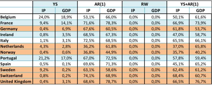
Belgium 24,0% 18,9% 53,1% 66,0% 0,0% 0,0% 50,1% 61,6% France 9,4% 14,1% 71,6% 78,3% 0,0% 0,0% 66,9% 73,9% Germany 0,4% 6,9% 67,6% 60,5% 0,0% 0,0% 61,8% 53,7% Ireland 0,8% 3,5% 68,5% 67,3% 0,0% 0,0% 47,0% 58,7%
Italy 1,1% 3,1% 72,5% 68,5% 0,0% 0,0% 65,5% 66,1%
Netherlands 4,3% 2,8% 36,2% 61,8% 0,0% 0,0% 37,0% 65,8% Norway 0,4% 0,6% 36,8% 44,9% 0,0% 0,0% 35,7% 40,2% Portugal 21,2% 17,0% 67,0% 72,5% 0,0% 0,0% 57,8% 59,4%
Spain 0,5% 0,1% 69,6% 71,3% 0,0% 0,0% 45,1% 65,2%
Sweden 9,2% 0,2% 63,1% 58,6% 0,0% 0,0% 62,4% 61,2% Switzerland 0,8% 0,2% 74,1% 68,9% 0,0% 0,0% 68,4% 60,7% United Kingdom 0,4% 3,1% 68,6% 78,7% 0,0% 0,0% 66,5% 76,7%
Table IS.15- Comparison of Several models for the whole period: Average of all time horizons – MAD
Table IS.16 - Comparison of Several models for Prior-2008: Average of all time horizons - MAD
The assessment of the relative strength of the YS model does not suffer major changes when
one analysis the MAD (see previous tables). When the comparison is made taking into
account the full sample, it becomes evident the significant gap existent between the
performance of the YS model and all the other benchmarks. The figure changes considerably
IP GDP IP GDP IP GDP IP GDP
Belgium 3,12 1,24 2,34 0,76 2,75 0,83 2,27 0,75
France 2,42 1,07 1,57 0,55 1,74 0,59 1,54 0,54
Germany 3,36 1,64 2,19 1,11 2,44 1,28 2,15 1,09
Ireland 6,35 3,67 4,37 1,69 5,17 1,81 4,63 2,01
Italy 3,62 1,78 2,10 0,81 2,32 0,87 2,09 0,88
Netherlands 2,93 1,62 2,70 0,98 3,39 1,10 2,49 0,77
Norway 4,29 1,82 3,46 1,54 4,38 1,96 3,43 1,48
Portugal 3,74 2,25 2,46 1,30 2,88 1,44 2,37 1,23
Spain 4,04 1,67 2,89 0,79 3,41 0,84 2,88 0,78
Sweden 3,66 1,62 2,62 1,24 2,99 1,47 2,51 1,10
Switzerland 3,51 1,93 1,91 0,82 2,09 0,87 1,92 0,84 United Kingdom 2,33 1,65 1,42 0,79 1,58 0,86 1,30 0,76
YS AR(1) RW YS+AR(1)
IP GDP IP GDP IP GDP IP GDP
Belgium 2,61 1,10 2,28 0,77 2,71 0,85 2,21 0,76
France 1,97 0,95 1,52 0,54 1,64 0,57 1,50 0,54
Germany 3,03 1,59 2,11 1,13 2,71 4,10 2,07 1,12
Ireland 6,15 2,97 4,32 1,71 5,18 1,79 4,57 2,04
Italy 2,90 1,26 2,08 0,80 2,25 0,86 2,08 0,80
Netherlands 2,49 1,24 2,63 1,31 1,64 2,78 2,38 0,74
Norway 3,91 1,73 3,26 1,00 2,27 3,54 3,20 1,47
Portugal 3,09 1,87 2,40 1,30 2,78 1,46 2,29 1,23
Spain 3,87 1,53 2,94 0,79 3,46 0,84 2,91 0,78
Sweden 3,05 1,78 2,55 1,30 5,18 2,91 2,45 1,14
Switzerland 2,88 1,35 1,91 0,83 2,25 2,06 1,89 0,81 United Kingdom 2,06 1,32 1,42 0,81 3,27 1,55 1,28 0,78
when the estimation is made for the period until 2008. At this stage, the YS has presented
more consistent achievements than the RW in one third of the cases, being a fairly superior
achievement noticed for the case of Sweden. Nevertheless, when confrontation is made for
both AR and AR+YS, one can still remark that the YS still falls short – contradicting the findings of Haubrich and Dombrosky (1996) for the USA, when an in-sample estimation is
carried out.
It is also expressive the behavior of the YS in the lagged output framework. Out of the 48
cases (i.e. for all countries, both dependent variables and sample periods), the YS improved
the predictive power of the AR model in only 7 occasions.
4.2.4) Diebold-Mariano test
In order to verify whether the difference in accuracy of the forecasts generated by the YS and
the other models is statistically significant, one performed the test proposed by Diebold and
Mariano (1995). This test is conducted from a time-t loss differential function defined as
– , i.e., the difference of the quadratic forecasts errors between models i and j
at time t. The null hypothesis assumes that both models have the same predictive accuracy. In
other words, one wishes to test whether the time-t loss differential function has expected
value equal to zero or E(dij;t) = 0. Assuming the null as true, one can build the Diebold
Mariano (DM) statistic:
̅̅̅̅
̂ ̅̅̅̅̅→ N(0,1)
where the ̅ ∑ can be defined as the mean of the loss differential observations and
̂ ̅̅̅̅ , a consistent estimator of its standard deviation. The last term was computed through the
procedure suggested by Newey and West (1987), which provides robust standard errors for
Satisfied these conditions, the DM statistic will follow a standard Normal distribution. In this
manner, by running an OLS regression (with Newey-West standard errors) of the loss
differential function on an intercept and observing its t-statistic, one can draw conclusions
about the difference in forecasts accuracy between models (see Diebold, 2014). Low values of
t-statistic/DM favor the veracity of the null hypothesis and, hence, suggest that models
provide, on average, the level of accuracy, whereas high values of t-statistic/DM demonstrate
evidences that one of the models often provides more proper forecasts than the other.
The Diebold-Mariano test was made to compare the performance of the YS model - for every
countries, time horizons and historical period - before the benchmarks. Table DM.1 presents a
summary result about the frequent in which the rejection of the null hypothesis was
confirmed, assuming a level of significance of 10%.
Table DM.1 – Frequency of discrepancy in accuracy prediction: comparison
between the YS model and the benchmarks - Diebold-Mariano test (Level of
significance: 10%) 12
The previous table corroborates the preceding conclusion that the forecasts obtained from the
YS model are often less accurate than the other models tested. By way of illustration, for the
full sample case that considers the GDP as the dependent variable, one remarks that the YS
has presented less precise predictions in about 70% of the cases; a result that showed to be
statistically significant. As it was also noticed in the analysis of tables IS.15 and IS.16, the
12
The critical values of the t-statistic used was tc = 1,66
IP GDP IP GDP
YS x AR(1) 45% 70% 36% 50%
YS x RW 45% 70% 36% 53%
YS x AR(1)+YS 46% 70% 36% 53%
gap in the performance of the YS is less prominent when the period after 2008 is included in
the sample.
A similar exercise was performed to assess the difference in forecasting accuracy between the
AR and the AR +YS. The outcomes were not surprising, if we take into consideration the
small divergence in the values of the MADs in tables IS.15 and IS.16: in none of the 192
cases tested, the YS showed to improve the forecasts of the autoregressive model.
4.2.5) In-Sample: The best fit that the YS models can achieve
Having analyzed the performance of models with different dependent variables, time horizons
forecasting periods and after a drastic overturn in the macroeconomic environments, one can
clearly conclude that the YS model has rather limited capability of prediction for an
individual set of European countries – the same conclusion was reached by Berk and van Bergeijk (2000) for an aggregate of the Euro Area. In spite of that, one may wish to observe at
which configurations of dependent variable, time horizon and historical period the YS model
yields the highest explanation power. The table IS.17, which summarizes these outcomes, was
built by a simple observation of the regressions with the greatest R-squared13.
13
Table IS.17 – Models with the best fit, per country
Several are the interesting aspects to be highlighted. Firstly, there is no clear evidence if the
yield spread is a more reliable leading indicator of real economic activity when this one is
measured either as IP or as real GDP. Secondly, the poor predictive power of the framework
analyzed should not be assigned to the last financial crisis. Thirdly, the models achieve peak
of their performance as of a medium time horizon (i.e, of 1-year ahead) and performs quite
badly for shorter periods (See table B5, in the appendix B). The same conclusion is reached
by Passaro (2007) for Germany and the USA and Nobili (2005) for countries of the Euro Area
as an aggregate. Hamilton and Kim’s (2002) finding for the USA that that the model starts
losing predictive power after 8 quarters in the future is not confirmed by most of the
economies here studied. Finally, the yield spread indicator does not convey any useful
information about Spain’s and Switzerland’s future economic growth (in all of the 32
regressions estimated, the R-squared barely overcomes 1%).
4.3) Out-of-sample estimation
Having extensively investigated the strength of the predictive power of the Yield Spread for
the in-sample procedure, one is going to assess the general performance of the model vis-à-vis
Dependent Variable Period Best time horizon
Belgium IP Prior to 2008 Medium + Long
France GDP Prior to 2008 Medium
Germany IP Whole period Medium + Long
Ireland IP Whole period Medium + Long
Italy GDP Prior to 2008 Long
Netherlands GDP Whole period NONE
Norway GDP Whole period Long
Portugal IP Prior to 2008 Medium + Long
Spain
Sweden GDP Whole period Medium
Switzerland
United Kingdom GDP Whole period Medium
to the same benchmarks of the previous section 4.2, but, this time, for an out-of-sample
estimation.
In the out-of-sample framework, the regressions take into consideration only the information
that was available at the moment - rather than the entire set of historical information (full
sample), as it is typically done in the in-sample estimation - that the forecasting was
conducted. In particular, for the YS model, one has computed the following equation:
YS’ model |
where It corresponds to the set of information available up to time t. It is important to highlight
that for all the models, the information set was decided to start in 1996Q4 and, hence, the
forecasts begun from the first quarter of 1997.
As it was done for the in-sample analysis, one resorted to both R-Squared and MAD as
assessment tools of YS model’s predictive quality.
A word of caution is needed for the case of the R-Squared. Due to the fact that the forecasts of
a given time horizon are generated by different models as time goes by (the parameters of the
model are re-estimated as a new information becomes available), the R-Squared may assume
negative values - feature that is impossible in our in-sample estimation14 - when the fit values
of the estimated model perform worse than the sample mean. As a result of that, electing the
estimation procedure (in and out of-sample) that yields the best fit becomes a meaningless
task. However, one can still compute the R-Squared as a manner of establishing comparisons
across countries within a certain period and to observe their behavior after the global of Crisis
2008. The outcomes of these estimations are provided by the following tables.
14
A linear model estimated by OLS containing an intercept and subject to no constraints must always provide a positive (or zero) value. See Wooldridge (2009).
Table OS.1- Comparison of Several models for the whole period: Average of all time horizons – Estimated R-squared
Table OS.2 - Comparison of Several models for Prior to 2008: Average of all time horizons - Estimated R-squared
Implementing the out-of-sample estimations does not change substantially the relative ranking
of the YS over the other models tested as it continues to demonstrate worse results when
compared with the top-performers. However, one may argue that the new estimation
procedure has contributed to enhance greatly the performance of the YS model, softening the
disparity with the benchmarks. This fit gain is especially meaningful when the regressions are
run until the year of 2008 (more on that in the next subsection).
IP GDP IP GDP IP GDP IP GDP
Belgium 44,4% 38,5% 52,3% 84,2% 58,7% 84,3% 64,9% 82,1% France 43,0% 32,6% 66,5% 85,9% 72,6% 84,9% 69,9% 83,3% Germany 50,3% 44,4% 63,4% 81,1% 70,4% 80,0% 71,0% 79,8% Ireland 19,9% 32,4% 51,8% 70,0% 51,4% 59,4% 60,6% 61,2%
Italy 27,6% 25,3% 68,0% 83,8% 76,9% 84,2% 72,3% 80,3%
Netherlands 39,0% 48,7% 34,6% 86,6% 56,4% 89,1% 65,7% 86,8% Norway 55,8% 42,1% 39,3% 77,3% 61,9% 67,9% 69,0% 73,8% Portugal 43,7% 52,0% 60,0% 87,0% 73,1% 85,6% 77,1% 82,9%
Spain 53,1% 32,5% 48,7% 85,5% 57,7% 83,9% 64,7% 83,2%
Sweden 62,6% 37,9% 61,8% 80,9% 77,1% 79,6% 76,7% 82,0% Switzerland 38,5% 28,5% 73,2% 91,3% 83,2% 95,6% 80,2% 88,0% United Kingdom -0,6% 40,6% 66,9% 1,4% 83,9% 1,5% 82,7% 1,2%
RW YS+AR(1)
AR(1) YS
IP GDP IP GDP IP GDP IP GDP
Belgium 61,8% 71,1% 72,4% 88,6% 63,2% 88,8% 71,3% 87,9% France 64,2% 68,4% 83,7% 89,7% 81,2% 89,0% 82,6% 88,0% Germany 62,8% 69,7% 84,4% 88,5% 83,6% 88,2% 83,2% 87,8% Ireland 42,6% 45,7% 67,7% 65,8% 51,2% 51,3% 63,1% 60,7%
Italy 64,4% 60,6% 84,5% 87,5% 82,4% 86,8% 83,0% 85,8%
Netherlands 69,9% 66,3% 75,2% 90,7% 67,8% 92,4% 74,9% 90,9% Norway 53,8% 77,9% 78,0% 82,9% 75,0% 75,2% 78,4% 82,4% Portugal 65,7% 63,8% 86,3% 90,1% 82,0% 87,3% 84,8% 86,9%
Spain 37,7% 65,3% 71,6% 90,7% 62,3% 90,2% 68,6% 89,3%
Sweden 71,9% 65,0% 83,8% 89,3% 81,0% 88,5% 83,7% 89,2% Switzerland 58,0% 75,8% 87,5% 94,0% 87,3% 95,4% 85,7% 93,2% United Kingdom 67,4% 73,0% 90,0% 90,3% 90,3% 90,6% 90,2% 89,8%