Small data oversampling: improving small data prediction accuracy using the geometric SMOTE algorithm

(1)

S

Small Data Oversampling

Improving small data prediction accuracy using

the Geometric SMOTE algorithm

Maria Lechleitner

Dissertation presented as the partial requirement for

obtaining a Master's degree in Data Science and Advanced

Analytics

(2)

NOVA Information Management School

Instituto Superior de Estatística e Gestão de Informação

Universidade Nova de Lisboa

Small Data Oversampling

Improving small data prediction accuracy using the Geometric SMOTE algorithm

Maria Lechleitner

Dissertation presented as the partial requirement for obtaining a Master's degree in Data

Science and Advanced Analytics

Advisor: Prof. Fernando José Ferreira Lucas Bação

(3)

Abstract

In the age of Big Data, many machine learning tasks in numerous industries are still restricted due to the use of small datasets. The limited availability of data often results in unsatisfactory prediction performance of supervised learning algorithms and, consequently, poor decision making. The current research work aims to mitigate the small dataset problem by artificial data generation in the pre-processing phase of the data analysis process. The oversampling technique Geometric SMOTE is applied to generate new training instances and enhance crisp data structures. Experimental results show a significant improvement on the prediction accuracy when compared with the use of original, small datasets and over other oversampling techniques such as Random Oversampling, SMOTE and Borderline SMOTE. These findings show that artificial data creation is a promising approach to overcome the problem of small data in classification tasks.

Keywords

(4)

List of Figures

Figure 1: Relationship between population, small sample and artificial data [Li and Lin, 2006] ... 2

Figure 2: Distribution of a small dataset [Tsai and Li, 2015] ... 3

Figure 3: MTD function [Li et al., 2007]... 4

Figure 4: Example of bootstrapping sets [Kuhn and Johnson, 2013] ... 5

Figure 5: Generation of noisy examples [Douzas and Bacao, 2019] ... 6

Figure 6: Generation of redundant examples [Douzas and Bacao, 2019] ... 7

Figure 7: Comparison of generated samples by SMOTE versus G-SMOTE [Douzas, 2019] ... 7

Figure 8: Example of positive class selection strategy [Douzas and Bacao, 2019] ... 10

Figure 9: Example of negative class selection strategy [Douzas and Bacao, 2019] ... 10

Figure 10: Example of combined selection strategy [Douzas and Bacao, 2019] ... 11

Figure 11: High-level experimental procedure ... 15

Figure 12: Mean ranking per classifier (Accuracy) ... 19

List of Tables

Table 1: Description of the datasets ... 13

Table 2: Results for mean cross validation scores of oversamplers ... 17

Table 3: Results for percentage difference between G-SMOTE and SMOTE ... 18

Table 4: Results for Friedman test ... 19

(6)

List of Abbreviations

BP Bootstrapping Procedure

BPNN Back-propagation Neural Network DNN Diffusion-Neural-Network

DT Decision Tree GB Gradient Boosting

GDPR General Data Protection Regulation G-MEAN Geometric Mean Score

G-SMOTE Geometric Synthetic Minority Oversampling Technique FVP Functional Virtual Population

KNN K-Nearest Neighbors LR Logistic Regression MTD Megea-Trend-Diffusion NB Naïve Bayes

NN Neural Network

SMOTE Synthetic Minority Oversampling Technique SVM Support Vector Machines

VC Vapnik-Chervonenkis VSG Virtual Sample Generation

(7)

1 Introduction

Insufficient size of datasets is a common issue in various supervised learning tasks [Niyogi et al., 1998], [Abdul Lateh et al., 2017]. The limited availability of training samples can be caused by different factors. First, data is becoming an increasingly expensive resource [Li et al., 2007] as the process to retain data is getting more complex due to strict privacy regulations such as the General Data Protection Regulation (GDPR) [European Commission, 2019]. Additionally, the small dataset problem can be found in numerous industries where organizations simply do not have access to a reasonable amount of data. For example, manufacturing industries are usually dealing with a small number of samples in early stages of product developments and health care organizations have to work with different kinds of rare diseases, where very few records are available [Abdul Lateh et al., 2017].

In machine learning, researchers are mainly concerned with the design and refinement of learning algo-rithms when aiming to improve prediction performance. However, increasing the sample size is often a more effective approach. A rule of thumb is that ”a dumb algorithm with lots and lots of data beats a clever one with modest amounts of it” [Domingos, 2012]. One of the reasons why even sophisticated algorithms do not perform well on small data is that small samples usually do not provide an unbiased representation of the reality. Generally, they are characterized by a loose data structure with many in-formation gaps, whereas bigger sample sets carry more observations to provide a complete picture of the underlying population. This lack of information negatively impacts the performance of machine learning algorithms [Lin et al., 2018]. Consequently, the knowledge gained from prediction models trained with small sample sizes is considered unreliable as well as imprecise and does not lead to a robust classification performance [Abdul Lateh et al., 2017].

Considering the size of data, there are two types of problems: First, the insufficiency of data belonging to one class (imbalance learning problem) for a binary or multi-class classification task and second, the size of the entire dataset (small dataset problem) for any classification or regression task [Sezer et al., 2014]. In both cases, small training samples affect the performance of machine learning models [Tsai and Li, 2008]. A theoretical definition of ”small” can be found in statistical learning theory by Vapnik. A sample size is seen as small, if the ratio between the number of training samples and Vapnik-Chervonenkis (VC) dimensions is less than 20. VC dimensions are determined as the maximum number of vectors that can be separated into two classes in all possible ways by a set of functions [Vapnik, 2008].

Under-representation of observations in the sample set can be solved in different ways. However, the use of synthetic data derived from existing (real) observations is a promising approach to the problem [Sezer et al., 2014]. Techniques to artificially add information by extending the sample size, and eventually improving the classification results of the algorithms, can translate into significant improvements in many application domains. However, it is important to note that virtual data samples are not necessarily representatives of the population, as they are artificially created. Taking this into consideration, the challenge in artificial data generation is to create data which extends the observed data without creating noise [Li and Lin, 2006]. Additionally, generating artificial data will only work if the initial sample is representative of the underlying population. Figure 1 shows the relationship between the entire population, a small sample and artificially created data.

(8)

Figure 1: Relationship between population, small sample and artificial data [Li and Lin, 2006]

The next sections will describe an effective way to tackle the small dataset problem. In chapter 2, the previously studied solutions such as Fuzzy Theories, Resampling Mechanisms and Oversampling Techniques are reviewed. Next, a detailed description of the proposed method G-SMOTE is presented in chapter 3. This is followed by the research methodology with the presentation of experimental data, evaluation measures, machine learning algorithms and experimental procedure in chapter 4 and the experimental results in chapter 5. Finally, the paper is concluded with an analysis of the experimental results and limitations as well as future research in chapter 6.

(9)

2 Related Work

Several data pre-processing methods to increase the data size have been presented by the research community. In this section, the three most important approaches are reviewed and the state-of-the-art to improve small dataset learning is reported. First, Fuzzy Theories will be presented which have historically been the most used approach to mitigate the small dataset problem. Next, Re-sampling Mechanisms such as bootstrapping techniques are highlighted. And finally, Oversampling Methods developed in the context of Imbalanced Learning are reviewed which can be a valuable option to increase the sample size of all classes given in a small dataset.

2.1 Fuzzy Theories

Many artificial sample generation techniques presented in the literature are based on fuzzy theories [Abdul Lateh et al., 2017]. The fuzzy set theory provides a strict mathematical framework to generalize the classical notion of a dataset. It gives a wider scope of applicability, especially in the fields of information processing and pattern classification [Zimmermann, 2010]. Based on this concept, several methods have emerged in the last decade to estimate or approximate functions which are generating more samples for sparse training sets.

The fundamental concept of fuzzy theories and artificially creating data is called Virtual Sample Gen-eration (VSG) and was originally proposed by [Niyogi et al., 1998]. The idea is to create additional observations within information gaps (see Figure 2) based on the current set of observed samples by using prior information. The introduction of virtual examples expands the effective training set size and can therefore help to mitigate the learning problem. [Niyogi et al., 1998] showed that the process of creating artificial samples is mathematically equivalent to incorporating prior knowledge. They demon-strate the concept on object recognition by mathematically transforming the views of 3D-objects. These new views are called virtual samples and its application extends information and results in successful generalization.

Figure 2: Distribution of a small dataset [Tsai and Li, 2015]

Based on Virtual Sample Generation, several closely related studies were developed for manufacturing environments. The first method to overcome scheduling problems due to the lack of data in early stages of manufacturing systems was the creation of a Functional Virtual Population (FVP) [Li et al., 2003]. The idea is to create a number of virtual samples within of a newly defined domain range. Although the method involves a highly manual process, the application of FVP dramatically improved the classification accuracy of a neural network.

The idea of fuzzifying information to extend a small dataset was also used to develop the Diffusion-Neural-Network (DNN) method [Huang and Moraga, 2004]. It combines the principle of information

(10)

diffusion by [Huang, 1997] with traditional Neural Networks to estimate functions. The information diffusion method partially fills the information gaps by using fuzzy theories to represent the similarities between samples and subsequently derive new ones.

The researchers [Li et al., 2006] further examined possible methods to learn scheduling knowledge with rare data in early stages of manufacturing systems. They developed a new data fuzzification technique called mega-fuzzification and combined it with a data trend estimation procedure to systematically expand the training data. The method fuzzifies a dataset as a whole and expands it in consideration of a previously defined data trend. The results of this study show high learning accuracy and denote the method as a reliable and applicable approach in the business marketplace. However, the difficulty in establishing the domain ranges and the lack of a theoretical basis explain its lack of popularity and limited interest.

In order to fully fill the information gaps, Mega-Trend-Diffusion (MTD) was introduced by [Li et al., 2007] which diffuses the sample set one by one. Their concept combines data trend estimation with a diffusion technique to estimate the domain range in order to avoid over-estimation. MTD diffuses a set of data instead of each sample individually. For example, two samples m and n (Figure 3) are diffused simultaneously into one function with their borders a and b. To estimate a and b, the algorithm takes the minimum and maximum values of the dataset and counts the number of data points which are smaller or greater than the average of the values. This method takes the domain range as well as data skewness into consideration when calculating new samples. The triangular shape of Figure 3 represents the membership function which shows the similarities between samples. M and n are the observations and their heights represent the possible values of the membership function.

Figure 3: MTD function [Li et al., 2007]

After estimating the domain range between a and b, samples are randomly produced within this area by using a common diffusion function. The artificial samples are then trained with a Back-propagation Neural Network (BPNN) like [Huang and Moraga, 2004] originally proposed. This technique is seen as an improvement of DNN and was initially developed to improve early flexible manufacturing sys-tem scheduling accuracy. In further research, MTD is widely used as a synthetic sample generation method and is recognized as an effective way to deal with small dataset problems [Abdul Lateh et al., 2017]. However, MTD only considers the data for independent attributes and does not deal with their relationships.

Also, a genetic algorithm based virtual sample generation was proposed. The method takes the rela-tionship among attributes into account and explores their integrated effects instead of examining them individually. The algorithm is performed in three steps: Initially, samples are randomly selected to determine the range of each attribute by using MTD functions. Next, a Genetic Algorithm is applied to find the most feasible virtual samples. Finally, the average error of these new samples is calculated. The results outperformed the ones using MTD and also showed better performance in prediction than in case of no generation of synthetic samples [Li and Wen, 2014].

The above presented fuzzy-based algorithms are limited on numerical attributes. If a dataset contains categorical features, a resampling mechanism, such as Bootstrap, can be considered. The basic concepts

(11)

of the Bootstrapping method and its application on the small data problem is described in the following section.

2.2 Resampling Mechanism

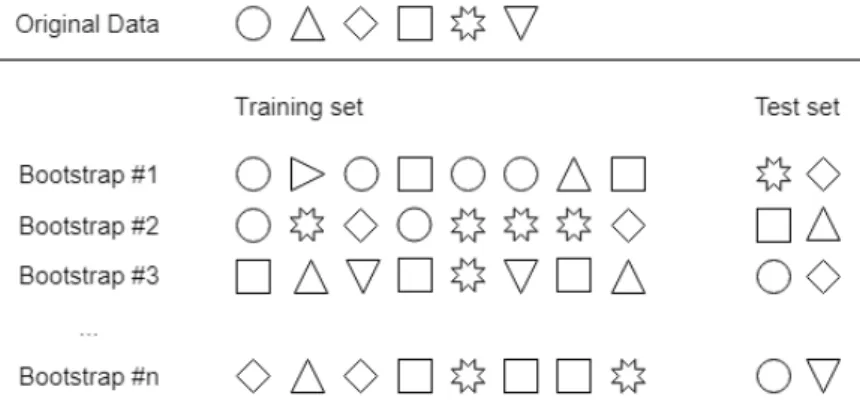
An alternative approach to fuzzy theories is the Bootstrapping Procedure (BP), which is the most well-known artificial sample generation method within resampling mechanisms [Abdul Lateh et al., 2017]. The main difference to the previously presented techniques is that BP creates new training sets by randomly resampling instances from the measured data with replacement [Efron and Tibshirani, 1993]. It allows the algorithms to use the same sample more than one time to gradually revise the identified patterns in order to improve predictive accuracy. Even though it can double the number of observations in a training set, Bootstrapping tends to cause over-fitting when applied to small data because it repetitively uses the same information. Also, since the amount of information provided by small data is minimal, any missing observation in the new, bootstrapped training set is a loss of valuable information (see Figure 4). As a result, Bootstrap can not be seen as an ideal solution to the small dataset problem, as it increases the number of training samples rather than the amount of (artificially generated) information [Tsai and Li, 2015], [Li et al., 2018]. However, [Iv˘anescu et al., 2006] applied BP in batch process industries where it was shown that it may help mitigate the small data problem.

Figure 4: Example of bootstrapping sets, where six samples are represented as symbols and are allocated to n possible subsets. The size of the subsets are increased using multiple instances of the original data. The data points which are not selected by the BP are used as a test set [Kuhn and Johnson, 2013].

In further studies of [Tsai and Li, 2008] and [Chao et al., 2011], the BP algorithm was applied to actually generate virtual samples in order to fill the information gaps. Instead of resampling observations, they execute the BP once for each input factor which results in a newly shuffled training set. After generating new instances, they are combined with the original dataset to train a neural network. The results show that this method significantly decreases the prediction error rate in modeling manufacturing systems as well as the prediction on radiotherapy of bladder cancer cells.

2.3 Oversampling Techniques

A different approach to fill information gaps is synthetic oversampling of the training set. Oversampling is an artificial data generation strategy originally developed in the context of machine learning to deal with the imbalanced learning problem. Therefore, its origin comes from a different research community than the fuzzy and resampling strategies presented above. Although fuzzy theories, resampling mechanisms and oversampling techniques are aiming to solve a similar problem, literature research shows that their proposed solutions had very few connections in the past.

(12)

In Imbalanced Learning, the classes of a given dataset are significantly skewed i.e. the dataset has a large number of observations in one class (majority class) and a very small number of observations in the other class (minority class). This constitutes a problem for the learning phase of the algorithm and results in low prediction accuracy for the minority class. In practice, the imbalanced dataset problem is a very common issue in supervised learning. Especially in the fields of fraud detection, product categorization and disease diagnosis, an imbalanced dataset is the norm rather than the exception [He and Ma, 2013].

2.3.1 SMOTE

There are several methods presented in the literature that tackle the imbalanced data problem. The most popular approach is the Synthetic Minority Oversampling Technique (SMOTE). SMOTE is based on the idea of k-nearest neighbors and linear interpolation as a data generation mechanism. More specifically, SMOTE proposes to form a line segment between neighboring minority class instances and to generate synthetic data between them [v. Chawla et al., 2002]. The algorithm is very popular due to its simplicity as well as its robustness. Numerous variations have been proposed based on SMOTE, increasing its status as the staple idea in oversampling for imbalanced learning problems [Fernandez et al., 2018]. However, SMOTE has some significant limitations when it comes to the sample generation process. In practice, the separation between majority and minority class areas is often not clearly definable. Thus, noisy samples may be generated when a minority sample lies in the region of the majority classes. Figure 5 presents a scenario where a minority instance is generated within the majority region (noisy sample).

Figure 5: Generation of noisy examples [Douzas and Bacao, 2019]

Furthermore, redundant instances may be generated within dense minority regions which results in not adding any relevant information to the classifier and may lead to over-fitting. Figure 6 demonstrates an example where a minority class instance is generated in a dense minority class. This new observation belongs to the same dense cluster as the original and is therefore less useful.

(13)

Figure 6: Generation of redundant examples [Douzas and Bacao, 2019]

Although SMOTE is recognized as an oversampling technique for imbalanced datasets, it can also be used for solving the small dataset problem. [Li et al., 2018] showed that SMOTE is able to fill the information gaps with synthetic samples. However, given its limitations, SMOTE does not achieve the best results within their study.

2.3.2 G-SMOTE

The novel data generation procedure Geometric SMOTE (G-SMOTE) has been presented with the objective to improve the above mentioned limitations of the SMOTE algorithm [Douzas and Bacao, 2019]. G-SMOTE can be seen as a substitute of SMOTE, enhanced by geometric properties. The main difference to SMOTE is that it expands the data generation area and prevents the creation of noise. Instead of connecting the minority sample and one of its nearest neighbors with a line segment (hypersphere), the instances are generated in a geometrical region (hyper-spheroid) around the minority sample. Furthermore, G-SMOTE is designed to avoid the generation of noisy samples by introducing the hyper-parameter selection strategy. Figure 7 demonstrates the distribution of artificially created samples by SMOTE versus G-SMOTE. With an increasing number of k-nearest neighbors, SMOTE tends to generate noisy samples, whereas G-SMOTE avoids this scenario.

Figure 7: Comparison of generated samples by SMOTE versus G-SMOTE when generating synthetic data based on three positive class instances [Douzas, 2019].

(14)

The study of [Douzas and Bacao, 2019] has performed an extensive comparison between G-SMOTE and SMOTE using 69 imbalanced datasets and several classifiers. The results show that G-SMOTE outper-forms SMOTE, Random Oversampling and the case of no oversampling across all datasets, classifiers and performance metrics.

(15)

3 Proposed Method

In the following section, G-SMOTE is presented as a novel data generation procedure for small datasets in the case of binary classification. Originally developed for the imbalanced learning problem, the algorithm is adapted in a way to not only resample the minority class, but the entire dataset independent on the class distribution.

3.1 G-SMOTE for the small dataset problem

As mentioned above, the G-SMOTE algorithm randomly generates artificial data within a geometrical region of the input space. The size of this area is derived from the distance of the selected sample to one of its nearest neighbors, whereas the shape is determined by the hyper-parameters called truncation factor and deformation factor. Additionally, the hyper-parameter selection strategy of G-SMOTE modifies the standard SMOTE selection process and also affects the size of the geometric region. Although the main concept can be adapted from the original method to the small dataset problem, the selection strategy requires some minor adjustments which will be described hereafter.

The hyper-parameter selection strategy αsel defines the radius of the surface point. This mechanism allows the positive or negative class area to expand into a direction where it prevents the algorithm from creating noisy samples. In G-SMOTE for small data, both classes are selected in two individual runs to introduce new observations. In the first run, a random sample called xsurf ace is selected which belongs to the positive class. Similarly, xsurf ace is assigned to the negative class samples in the second run. Both runs are based on the defined selection strategy where αsel can have three different values: positive class selection Spos, negative class selection Snegand combined selection Scom. In the first run of the algorithm, a positive sample is selected and the data generation process is started. After increasing the instances in the positive class, a second run is initiated to randomly choose a negative class example and repeat the data generation process inversely.

The class selection strategies are described in regard to the first run, where a positive sample is randomly selected.

(a) Positive class selection

With the hyper-parameter selection strategy = ’positive’, a second positive class sample is selected as one of the k-nearest neighbors. This indicates that the selection strategy is based only on the positive class and works like the selection strategy of SMOTE. As SMOTE may lead to the generation of data penetrating the opposite class area, this drawback also applies on the selection strategy here.

(16)

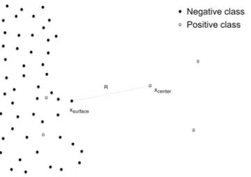
Figure 8: Example of positive class selection strategy: A positive class instance is defined as the center and one of its k = 4 positive class nearest neighbors is selected as the surface point. The radius R is equal to the distance of these instances [Douzas and Bacao, 2019].

(b) Negative class selection

When selection strategy = ’negative’, a negative sample is selected as the nearest class neighbor. This scenario prevents the algorithm from creating noisy samples. More specifically, as the radius is drawn from the selected positive class instance to the nearest neighbor of the negative class, it does not allow the data generation mechanism to penetrate the opposite area.

Figure 9: Example of negative class selection strategy: A positive class instance is defined as the center and its closest negative class neighbor is selected as the surface point. The radius R is defined to be equal to the distance of these instances [Douzas and Bacao, 2019].

(c) Combined selection

The combined selection strategy initially applies the positive and negative selection strategies. Once xpos and xneg are identified, the point with the minimum distance to the center xcenter is defined as the surface point xsurf ace. Figure 10 presents an example when xsurf ace is identified as a negative class instance.

(17)

Figure 10: The closest point xneg to the center positive class sample xcenter is identified as the surface point xsurf acesince it is closer to the center than the selected instance xpos from the k nearest positive class neighbors of the center [Douzas and Bacao, 2019].

3.2 Adapted G-SMOTE algorithm

The inputs of the G-SMOTE algorithm are the positive Spos and negative class samples Sneg, the trunca-tion factor, deformatrunca-tion factor and selectrunca-tion strategy as well as the number of generated samples for the positive class Npos and for the negative class Nneg. The number of generated samples preserves the class distribution in the re-sampled dataset. The adapted G-SMOTE algorithm can be generally described in the following steps:

1. An empty set Sgen is initialized. Sgen will be populated with artificial data from both classes. 2. The Spos elements are shuffled and the process described below is repeated Npos times until Npos

artificial points have been generated.

2.1. A positive class instance xcenter is selected randomly as the center of the geometric region. 2.2. Depending on the values of αsel (positive, negative or combined), this step results in a

ran-domly selected sample xsurf ace which belongs to either Spos or Sneg

2.3. A random point xgenis generated inside the hyper-spheroid centred at xcenter. The major axis of the hyper-spheroid is defined by xsurf ace- xcenterwhile the permissible data generation area and the rest of geometric characteristics are determined by the hyper-parameters truncation factor and deformation factor.

(a) The truncation factor αtrunc defines the degree of truncation that is applied to the ge-ometric area and can be specified between zero and one, where truncation factor = 0.0 corresponds to a circle and truncation factor = 1.0 becomes a half-hypersphere around the selected sample.

(b) The formation of the area is defined by the so-called deformation factor. If the parameter of the deformation factor is equal to 0, the data generation area obtains a circle. On the opposite, if the parameter is set to 1, the area deforms to a line segment.

(18)

3. Step 2 is repeated using the substitution pos ↔ neg until Nnegartificial points have been generated. The above description of the algorithm excludes mathematical formulas and details which can be found in [Douzas and Bacao, 2019].

(19)

4 Research Methodology

The main objective of this work is to compare G-SMOTE with other oversampling techniques when it comes to the small dataset problem. Therefore, a variety of datasets, evaluation measures and classifiers is used to evaluate the performance. A description of this set-up, the experimental procedure as well as the software implementation is provided in this section.

4.1 Experimental Data

The performance of G-SMOTE is tested with ten different datasets, which are retrieved from UCI Machine Learning Repository [Dua and Graff, 2019]. The focus on the selection of the data lies on binary classification problems with a balanced distribution of the two classes. The type of data is numerical. In order to assure generalizability of the results, the datasets include different topics such as health care, finance, business and physics as well as different sample sizes. Details of the datasets are presented in the following table:

Dataset Number of samples Number of attributes Area

Arcene 900 10.000 Health Care

Audit 776 18 Business

Banknote Authentication 1.372 5 Finance

Spambase 4.610 57 Business

Breast Cancer 699 10 Health Care

Indian Liver Patient 583 10 Health Care

Ionosphere 351 34 Physics

MAGIC Gamma Telescope 19.020 11 Physics

Musk 6.598 168 Physics

Parkinsons 197 23 Health Care

Table 1: Description of the datasets

4.2 Evaluation Measures

To evaluate the performance of G-SMOTE, the experiment includes two different measures: accuracy and geometric mean.

Accuracy is used as one of the most common metrics for evaluating classification models [Hossin and Sulaiman, 2015]. Accuracy measures the ratio of correct predictions over the total number of instances evaluated. The accuracy metric can be stated mathematically as

Accuracy = T P + T N T P + T N + F P + F N

where T P/T N denote the number of correctly classified positive and negative instances, while F P/F N denote the number of misclassified negative and positive instances, respectively. The accuracy metric might be negligible for datasets with a significant disparity between the number of positive and negative labels. As pointed out by many studies, accuracy has limitations in the discrimination process, since rare classes have a small impact on the measure compared to majority classes.

(20)

mean score (G-Mean) is included as a second measure. G-Mean measures the trade-off between sensitivity (true positive rate) and specificity (true negative rate) by the following:

G − M ean =psensitivity × specif icity = r

T P T P + F N ×

T N T N + F P

The objective of both measures is to be maximized since a classifier is performing well if it provides high classification accuracy and a high ratio of positive and negative accuracy [Han et al., 2012].

4.3 Machine Learning Algorithms

The experiment is conducted using several classifiers to make sure the results are not dependent on the machine learning algorithm. The following four classifiers are applied: Logistic Regression (LR) [McCullagh and Nelder, 2019], K-Nearest Neighbors (KNN) [Cover and Hart, 1967], Decision Tree (DT) [Salzberg, 1994] and Gradient Boosting (GB) [Friedman, 2001].

4.4 Experimental Procedure

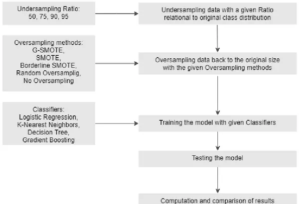
The main concept of the experimental procedure is to randomly undersample the datasets presented in Table 1, increase them artificially with different oversampling methods and compare the results with the original dataset which is considered to be the benchmark. This method enables a direct comparison between the quality of the artificial generated sample set and the observed data. In order to evaluate if the proposed method can improve artificial data generation, the study compares G-SMOTE with Random Oversampling, SMOTE and Borderline SMOTE. To undersample the data, a ratio of 50, 75, 90 and 95 percent of the original dataset is used. For example, with an undersampling ratio of 95 percent, only five percent of the original data are assigned as a base to apply the oversampling mechanism. This approach aims to provide an understanding of the classification performance as the size of the dataset diminishes.

(21)

Figure 11: High-level experimental procedure

A k-fold cross-validation is used as a technique for assessing the performance of the models for each combination of oversampling method and classifiers. The dataset D is randomly split into k subsets (folds) D1, D2, . . . Dkof approximately equal size. Each fold is used as a validation set and the remaining folds are used to train the model with k iterations. This procedure is repeated until each k have been used as a validation set [Han et al., 2012]. Based on this technique, the experiment is conducted in the following steps within one iteration:

1. Splitting dataset into k-fold cross-validation sets

2. The k − 1 folds are under-sampled using an undersampling ratio 50, 75, 90 and 95, corresponding to the percentage of the dataset that is removed.

3. Over-sampling is applied to the under-sampled data of the previous steps that increases their size and class distribution back to the initial.

4. The re-sampled data of the previous step are used to train the classifiers. 5. The classifiers are evaluated on the remaining fold of step 1.

This procedure is repeated three times and the on average highest cross validation score for each com-bination of dataset, classifier, oversampler and evaluation metric is reported.

In order to confirm the statistical significance of the experimental results, the Friedman test [Sheldon et al., 1996] as well as the Holm test [Demsar, 2006] are applied. The Friedman test is a non-parametric procedure to test hypothesis on ordinal scaled variables. Additionally, it can also be applied with interval data when normality and homogeneity assumption does not hold. The Friedman test is used to evaluate the data generation algorithms on each dataset separately. Ranking scores are assigned to each oversampling method with scores of 1 to 5 for the best and worst performing methods, respectively. The procedure compares the average ranks of the algorithms under the null hypothesis, which states that

(22)

the independent variable has no effect on the dependent variable. In this experimental set-up, the null hypothesis assumes that all five algorithms show identical performance independent of the oversampling method and evaluation metric used. If the null-hypothesis is rejected to our favour, we proceed with the Holm test.

The Holm test acts as a post-hoc test for the Friedman test for controlling the family-wise error rate when all algorithms are compared to a control method and not between themselves. This non-parametric test is very powerful in situations where one wants to evaluate whether a newly proposed method is better than existing ones. The control method in this set-up is the proposed G-SMOTE method and is tested under the null hypothesis whether G-SMOTE yields an improved performance over other oversampling methods.

4.5 Software Implementation

The implementation of the experimental procedure is based on Python programming language using the Scikit-Learn library [Pedregosa et al., 2011]. All functions, algorithms, experiments and results reported are provided at the GitHub repository of the project. They can be adjusted and implemented in comparative studies as the procedure is fully integrated with the Scikit-Learn ecosystem.

(23)

5 Results and Discussion

In this section the performance of the different oversampling methods and the results of the statistical tests are presented.

5.1 Comparative Presentation

The mean cross validation scores and the standard error per classifier across all datasets are shown in Table 2. The scores are presented for each undersampling ratio to evaluate the performance of the methods as the dataset size diminishes. We also include the benchmark method that represents the original dataset without applying undersampling before training the algorithm. This sample set is expected to obtain the best results by design.

Ratio Classifier Metric NONE RANDOM SMOTE B-SMOTE G-SMOTE BENCHMARK

50 LR ACCURACY 0.91 ± 0.03 0.91 ± 0.03 0.91 ± 0.02 0.91 ± 0.03 0.92 ± 0.02 0.92 ± 0.02 50 LR G-MEAN 0.88 ± 0.04 0.88 ± 0.04 0.89 ± 0.04 0.89 ± 0.04 0.89 ± 0.04 0.90 ± 0.04 50 KNN ACCURACY 0.88 ± 0.03 0.88 ± 0.03 0.89 ± 0.03 0.88 ± 0.03 0.89 ± 0.03 0.90 ± 0.03 50 KNN G-MEAN 0.84 ± 0.04 0.85 ± 0.04 0.86 ± 0.04 0.85 ± 0.04 0.86 ± 0.04 0.87 ± 0.04 50 DT ACCURACY 0.88 ± 0.04 0.88 ± 0.04 0.88 ± 0.04 0.88 ± 0.04 0.90 ± 0.03 0.90 ± 0.03 50 DT G-MEAN 0.86 ± 0.05 0.86 ± 0.05 0.87 ± 0.05 0.87 ± 0.05 0.89 ± 0.04 0.89 ± 0.03 50 GBC ACCURACY 0.91 ± 0.04 0.92 ± 0.03 0.92 ± 0.03 0.91 ± 0.04 0.93 ± 0.03 0.94 ± 0.02 50 GBC G-MEAN 0.90 ± 0.04 0.90 ± 0.04 0.91 ± 0.03 0.90 ± 0.04 0.92 ± 0.03 0.93 ± 0.03 75 LR ACCURACY 0.90 ± 0.03 0.89 ± 0.03 0.89 ± 0.03 0.89 ± 0.03 0.90 ± 0.03 0.92 ± 0.02 75 LR G-MEAN 0.86 ± 0.05 0.86 ± 0.05 0.87 ± 0.04 0.87 ± 0.04 0.87 ± 0.04 0.90 ± 0.04 75 KNN ACCURACY 0.86 ± 0.04 0.86 ± 0.04 0.87 ± 0.04 0.85 ± 0.04 0.87 ± 0.04 0.90 ± 0.03 75 KNN G-MEAN 0.80 ± 0.06 0.82 ± 0.05 0.84 ± 0.04 0.83 ± 0.05 0.84 ± 0.04 0.87 ± 0.04 75 DT ACCURACY 0.86 ± 0.05 0.86 ± 0.05 0.86 ± 0.05 0.85 ± 0.06 0.89 ± 0.04 0.90 ± 0.03 75 DT G-MEAN 0.83 ± 0.06 0.84 ± 0.05 0.84 ± 0.06 0.83 ± 0.06 0.86 ± 0.05 0.89 ± 0.03 75 GBC ACCURACY 0.87 ± 0.05 0.88 ± 0.05 0.88 ± 0.05 0.88 ± 0.05 0.90 ± 0.04 0.94 ± 0.02 75 GBC G-MEAN 0.85 ± 0.06 0.85 ± 0.06 0.86 ± 0.05 0.85 ± 0.06 0.89 ± 0.04 0.93 ± 0.03 90 LR ACCURACY 0.86 ± 0.04 0.86 ± 0.04 0.86 ± 0.04 0.85 ± 0.04 0.87 ± 0.04 0.92 ± 0.02 90 LR G-MEAN 0.81 ± 0.06 0.82 ± 0.06 0.82 ± 0.06 0.82 ± 0.05 0.83 ± 0.06 0.90 ± 0.04 90 KNN ACCURACY 0.81 ± 0.05 0.82 ± 0.05 0.82 ± 0.05 0.81 ± 0.05 0.83 ± 0.05 0.90 ± 0.03 90 KNN G-MEAN 0.69 ± 0.10 0.76 ± 0.07 0.78 ± 0.06 0.74 ± 0.09 0.78 ± 0.06 0.87 ± 0.04 90 DT ACCURACY 0.84 ± 0.05 0.83 ± 0.05 0.83 ± 0.06 0.83 ± 0.05 0.87 ± 0.04 0.90 ± 0.03 90 DT G-MEAN 0.81 ± 0.06 0.81 ± 0.06 0.80 ± 0.06 0.80 ± 0.06 0.84 ± 0.05 0.89 ± 0.03 90 GBC ACCURACY 0.84 ± 0.06 0.84 ± 0.06 0.84 ± 0.06 0.84 ± 0.05 0.88 ± 0.04 0.94 ± 0.02 90 GBC G-MEAN 0.82 ± 0.06 0.81 ± 0.06 0.81 ± 0.07 0.81 ± 0.06 0.86 ± 0.05 0.93 ± 0.03 95 LR ACCURACY 0.83 ± 0.05 0.83 ± 0.05 0.83 ± 0.05 0.83 ± 0.04 0.84 ± 0.05 0.92 ± 0.02 95 LR G-MEAN 0.75 ± 0.08 0.76 ± 0.07 0.76 ± 0.07 0.77 ± 0.07 0.76 ± 0.08 0.90 ± 0.04 95 KNN ACCURACY 0.79 ± 0.05 0.79 ± 0.05 0.81 ± 0.05 0.79 ± 0.05 0.81 ± 0.05 0.90 ± 0.03 95 KNN G-MEAN 0.60 ± 0.13 0.69 ± 0.09 0.71 ± 0.09 0.74 ± 0.06 0.73 ± 0.07 0.87 ± 0.04 95 DT ACCURACY 0.81 ± 0.05 0.81 ± 0.05 0.82 ± 0.05 0.81 ± 0.05 0.85 ± 0.05 0.90 ± 0.03 95 DT G-MEAN 0.77 ± 0.06 0.78 ± 0.06 0.78 ± 0.06 0.78 ± 0.06 0.81 ± 0.06 0.89 ± 0.03 95 GBC ACCURACY 0.82 ± 0.05 0.83 ± 0.05 0.83 ± 0.05 0.82 ± 0.05 0.85 ± 0.05 0.94 ± 0.02 95 GBC G-MEAN 0.77 ± 0.07 0.78 ± 0.07 0.78 ± 0.07 0.78 ± 0.07 0.81 ± 0.07 0.93 ± 0.03

Table 2: Results for mean cross validation scores of oversamplers (NONE corresponds to No Oversam-pling, RANDOM to Random Oversampling and B-SMOTE to Borderline SMOTE)

The above table shows that G-SMOTE outperforms almost all oversampling methods used for both, accuracy and g-mean metrics, on all classifiers. The highest score in the experiment is achieved by G-SMOTE with Gradient Boosting classifier and an average accuracy of 93%. The undersampling ratio in this case is 50% of the entire dataset. Throughout the scores we can observe that all oversampling

(24)

methods have a better performance as the datasets increase their size i.e. the undersampling ratio gets smaller.

The scores of G-SMOTE are very similar to the ones of the Benchmark method which implies that the proposed method is able to artificially establish a representative dataset. Of all oversampling methods, the artificial data created by G-SMOTE is the one closest to the observed data of the benchmark method.

Table 3 presents the mean and standard error of percentage difference between G-SMOTE and SMOTE. It shows that G-SMOTE performs better on average than SMOTE in almost every combination of ratio, classifier and metric.

Ratio Classifier Metric Difference

50 LR ACCURACY 0.27 ± 0.11 50 LR G-MEAN -0.52 ± 0.56 50 KNN ACCURACY 0.35 ± 0.24 50 KNN G-MEAN 0.51 ± 0.51 50 DT ACCURACY 2.56 ± 1.15 50 DT G-MEAN 2.73 ± 1.26 50 GBC ACCURACY 1.72 ± 0.93 50 GBC G-MEAN 1.57 ± 0.82 75 LR ACCURACY 0.58 ± 0.29 75 LR G-MEAN 0.35 ± 0.18 75 KNN ACCURACY 0.64 ± 0.60 75 KNN G-MEAN 0.62 ± 0.93 75 DT ACCURACY 4.23 ± 2.28 75 DT G-MEAN 4.24 ± 2.27 75 GBC ACCURACY 3.06 ± 2.02 75 GBC G-MEAN 3.44 ± 2.39 90 LR ACCURACY 1.19 ± 0.44 90 LR G-MEAN 1.10 ± 0.45 90 KNN ACCURACY 1.06 ± 1.31 90 KNN G-MEAN 0.53 ± 1.31 90 DT ACCURACY 5.78 ± 2.64 90 DT G-MEAN 5.45 ± 2.69 90 GBC ACCURACY 5.18 ± 2.53 90 GBC G-MEAN 7.46 ± 2.95 95 LR ACCURACY 1.20 ± 0.47 95 LR G-MEAN -0.80 ± 2.78 95 KNN ACCURACY 0.05 ± 0.26 95 KNN G-MEAN 6.75 ± 6.95 95 DT ACCURACY 3.51 ± 1.38 95 DT G-MEAN 4.09 ± 1.65 95 GBC ACCURACY 3.67 ± 2.16 95 GBC G-MEAN 4.15 ± 2.28

Table 3: Results for percentage difference between G-SMOTE and SMOTE

As explained in section 4, a ranking score in the range 1 to 5 is assigned to each oversampling method. The mean ranking of all oversampling methods across the datasets is presented in the following figure:

(25)

Figure 12: Mean ranking per classifier (Accuracy)

G-SMOTE is ranked on the top place when comparing with SMOTE, Borderline SMOTE, Random Oversampling and No Oversampling. Additionally, G-SMOTE slightly outperforms the Benchmark method using the classifiers Logistic Regression and Decision Tree in the mean ranking.

5.2 Statistical Analysis

To confirm the significance of the above presented results we apply the Friedman test as well as the Holm Test on the results. The application of the Friedman test is presented below:

Classifier Metric p-value Significance

LR ACCURACY 1.2e-11 True

LR G-MEAN 6.9e-08 True

KNN ACCURACY 2.7e-12 True

KNN G-MEAN 3.5e-13 True

DT ACCURACY 2.9e-12 True

DT G-MEAN 6.7e-11 True

GBC ACCURACY 4.9e-11 True

GBC G-MEAN 1.7e-09 True

Table 4: Results for Friedman test

(26)

the oversamplers do not perform similarly in the mean rankings across all classifiers and evaluation metrics.

The Holm’s method is applied to adjust the p-values of the paired difference test with G-SMOTE algorithm as the control method. The results are shown in table 5:

Classifier Metric NONE RANDOM SMOTE B-SMOTE

LR ACCURACY 2.9e-04 7.6e-05 2.9e-04 5.4e-05

LR G-MEAN 2.1e-01 2.1e-01 1.0e+00 1.0e+00

KNN ACCURACY 2.7e-05 7.8e-08 1.4e-01 1.8e-04

KNN G-MEAN 1.1e-02 3.3e-04 2.9e-01 2.9e-01

DT ACCURACY 1.5e-05 1.5e-05 4.8e-05 3.3e-05

DT G-MEAN 1.3e-05 4.4e-05 4.4e-05 4.4e-05

GBC ACCURACY 2.2e-04 2.9e-04 5.8e-04 1.8e-04

GBC G-MEAN 1.8e-04 3.9e-04 7.3e-04 7.3e-04

Table 5: Adjusted p-values using Holm test (B-SMOTE corresponds to Borderline SMOTE)

At a significance level of a = 0.05 the null hypothesis of the Holm’s test is rejected for a high number of combinations, indicating that the proposed method outperforms other methods in most cases.

(27)

6 Conclusions

The final chapter concludes this work with a summary and points out limitations as well as future research.

6.1 Summary

This research illustrates an effective solution to mitigate the small dataset problem in binary classification tasks. The oversampling algorithm G-SMOTE has the ability to represent the underlying population of a small sample very well and generates high quality artificial samples which improves prediction accuracy of the classifiers used in the experiment. This improvement in the forecasting performance of G-SMOTE relates to its capability of increasing the diversity of generated instances while generating artificial samples in safe areas of the input space. The successful implementation of this oversampling method in imbalance data problems can be translated into small dataset problems, which shows a lot of potential for possible linkage of these research areas in the future. The G-SMOTE implementation is available on GitHub and as an open source project.

6.2 Limitations and future research

The experiments are carried out on simple binary classification problems. Nevertheless, the application of the adapted G-SMOTE for multi-class classification tasks is an option. Future work can include the case of multi-class based on the binarization of the problem through the one-vs-all approach to evaluate the performance of G-SMOTE on small data with more than two classes. Additionally, the application of the adapted G-SMOTE on regression tasks can be performed. However, this is a topic for future research as the G-SMOTE algorithm requires an extensive modification in order to be applied to regression tasks.

A restriction of this work is the selection of balanced datasets only. Although it allows the work to be more generally applicable, it would be interesting to evaluate on how the G-SMOTE for small data performs on more imbalanced datasets. The adapted G-SMOTE can be executed on the original, imbalanced dataset or an alternative is to study the effect of first, balancing the dataset and then increasing the entire sample set with G-SMOTE for small data.

Furthermore, the experiment was tested on four commonly used classifiers: Logistic Regression (LR), K-Nearest Neighbors (KNN), Decision Tree (DT) and Gradient Boosting (GB). In order to enhance the validity of the results, other methods can be included such as Neural Networks (NN), Support Vector Machines (SVM) or Naive Bayes (NB).

(28)

References

[Abdul Lateh et al., 2017] Abdul Lateh, M., Kamilah Muda, A., Izzah Mohd Yusof, Z., Azilah Muda, N., and Sanusi Azmi, M. (2017). Handling a small dataset problem in prediction model by employ artificial data generation approach: A review. Journal of Physics: Conference Series, 892:012016. [Chao et al., 2011] Chao, G.-Y., Tsai, T.-I., Lu, T.-J., Hsu, H.-C., Bao, B.-Y., Wu, W.-Y., Lin, M.-T.,

and Lu, T.-L. (2011). A new approach to prediction of radiotherapy of bladder cancer cells in small dataset analysis. Expert Systems with Applications, 38(7):7963–7969.

[Cover and Hart, 1967] Cover, T. and Hart, P. (1967). Nearest neighbor pattern classification. IEEE Transactions on Information Theory, 13(1):21–27.

[Demsar, 2006] Demsar, J. (2006). Statistical comparisons of classifiers over multiple data sets. Journal of Machine Learning Research, 7:1–30.

[Domingos, 2012] Domingos, P. (2012). A few useful things to know about machine learning. Commu-nications of the ACM, 55(10):78.

[Douzas, 2019] Douzas, G. (2019). Data generation mechanism: Avoid-ing the generation of noisy samples: Available at https://geometric-smote.readthedocs.io/en/latest/auto examples/plot data generation mechanism.html#sphx-glr-auto-examples-plot-data-generation-mechanism-py. last checked on nov 30, 2019.

[Douzas and Bacao, 2019] Douzas, G. and Bacao, F. (2019). Geometric smote a geometrically enhanced drop-in replacement for smote. Information Sciences, 501:118–135.

[Dua and Graff, 2019] Dua, D. and Graff, C. (2019). Uci machine learning repository: Available at http://archive.ics.uci.edu/ml. last checked on nov 30, 2019.

[Efron and Tibshirani, 1993] Efron, B. and Tibshirani, R. (1993). An introduction to the bootstrap, volume 57 of Monographs on statistics and applied probability. Chapman & Hall, New York.

[European Commission, 2019] European Commission (2019). Data protection under gdpr: Available at https://europa.eu/youreurope/business/dealing-with-customers/data-protection/data-protection-gdpr/index en.htm. last checked on nov 30, 2019.

[Fernandez et al., 2018] Fernandez, A., Garcia, S., Herrera, F., and v. Chawla, N. (2018). Smote for learning from imbalanced data: Progress and challenges, marking the 15-year anniversary. Journal of Artificial Intelligence Research, 61:863–905.

[Friedman, 2001] Friedman, J. H. (2001). Greedy function approximation: A gradient boosting machine. The Annals of Statistics, 29(5):1189–1232.

[Han et al., 2012] Han, J., Kamber, M., and Pei, J. (2012). Data mining: Concepts and techniques. Morgan Kaufmann and Elsevier Science, Waltham, MA, 3rd ed. edition.

[He and Ma, 2013] He, H. and Ma, Y., editors (2013). Imbalanced learning: Foundations, algorithms, and applications. IEEE Press, Wiley, Hoboken, NJ.

[Hossin and Sulaiman, 2015] Hossin, M. and Sulaiman, M. N. (2015). A review on evaluation metrics for data classification evaluations. International Journal of Data Mining & Knowledge Management Process, 5(2):01–11.

(29)

[Huang, 1997] Huang, C. (1997). Principle of information diffusion. Fuzzy Sets and Systems, 91(1):69–90. [Huang and Moraga, 2004] Huang, C. and Moraga, C. (2004). A diffusion-neural-network for learning

from small samples. International Journal of Approximate Reasoning, 35(2):137–161.

[Iv˘anescu et al., 2006] Iv˘anescu, V. C., Bertrand, J. W. M., Fransoo, J. C., and Kleijnen, J. P. C. (2006). Bootstrapping to solve the limited data problem in production control: an application in batch process industries. Journal of the Operational Research Society, 57(1):2–9.

[Kuhn and Johnson, 2013] Kuhn, M. and Johnson, K. (2013). Applied predictive modeling. Springer, New York.

[Li et al., 2003] Li, D.-C., Chen, L.-S., and Lin, Y.-S. (2003). Using functional virtual population as as-sistance to learn scheduling knowledge in dynamic manufacturing environments. International Journal of Production Research, 41(17):4011–4024.

[Li et al., 2018] Li, D.-C., Lin, W.-K., Chen, C.-C., Chen, H.-Y., and Lin, L.-S. (2018). Rebuilding sample distributions for small dataset learning. Decision Support Systems, 105:66–76.

[Li and Lin, 2006] Li, D.-C. and Lin, Y.-S. (2006). Using virtual sample generation to build up man-agement knowledge in the early manufacturing stages. European Journal of Operational Research, 175(1):413–434.

[Li and Wen, 2014] Li, D.-C. and Wen, I.-H. (2014). A genetic algorithm-based virtual sample generation technique to improve small data set learning. Neurocomputing, 143:222–230.

[Li et al., 2006] Li, D.-C., Wu, C.-S., Tsai, T.-I., and Chang, F. M. (2006). Using mega-fuzzification and data trend estimation in small data set learning for early fms scheduling knowledge. Computers & Operations Research, 33(6):1857–1869.

[Li et al., 2007] Li, D.-C., Wu, C.-S., Tsai, T.-I., and Lina, Y.-S. (2007). Using mega-trend-diffusion and artificial samples in small data set learning for early flexible manufacturing system scheduling knowledge. Computers & Operations Research, 34(4):966–982.

[Lin et al., 2018] Lin, L.-S., Li, D.-C., Chen, H.-Y., and Chiang, Y.-C. (2018). An attribute extending method to improve learning performance for small datasets. Neurocomputing, 286:75–87.

[McCullagh and Nelder, 2019] McCullagh, P. and Nelder, J. A. (2019). Generalized Linear Models. Routledge.

[Niyogi et al., 1998] Niyogi, P., Girosi, F., and Poggio, T. (1998). Incorporating prior information in machine learning by creating virtual examples. Proceedings of the IEEE, 86(11):2196–2209.

[Pedregosa et al., 2011] Pedregosa, F., Varoquaux, G., Gramfort, A., Michel, V., Thirion, B., Grisel, O., Blondel, M., Prettenhofer, P., Weiss, R., Dubourg, V., Vanderplas, J., Passos, A., Cournapeau, D., Brucher, M., Perrot, M., and Duchesnay, E. (2011). Scikit-learn: Machine learning in python. Journal of Machine Learning Research 12 (2011) 2825-2830, 12.

[Salzberg, 1994] Salzberg, S. L. (1994). C4.5: Programs for machine learning by j. ross quinlan. morgan kaufmann publishers, inc., 1993. Machine Learning, 16(3):235–240.

(30)

pro-ducing synthetic samples by fuzzy c-means for limited number of data in prediction models. Applied Soft Computing, 24:126–134.

[Sheldon et al., 1996] Sheldon, M. R., Fillyaw, M. J., and Thompson, W. D. (1996). The use and interpretation of the friedman test in the analysis of ordinal-scale data in repeated measures designs. Physiotherapy Research International, 1(4):221–228.

[Tsai and Li, 2015] Tsai, C.-H. and Li, D.-C., editors (2015). Improving Knowledge Acquisition Capa-bility of M5’ Model Tree on Small Datasets. IEEE.

[Tsai and Li, 2008] Tsai, T.-I. and Li, D.-C. (2008). Utilize bootstrap in small data set learning for pilot run modeling of manufacturing systems. Expert Systems with Applications, 35(3):1293–1300.

[v. Chawla et al., 2002] v. Chawla, N., Bowyer, K. W., Hall, L. O., and Kegelmeyer, W. P. (2002). Smote: Synthetic minority over-sampling technique. Journal of Artificial Intelligence Research, 16:321–357.

[Vapnik, 2008] Vapnik, V. N. (2008). The nature of statistical learning theory. Statistics for engineering and information science. Springer, New York, 2. ed., 6. print edition.

[Zimmermann, 2010] Zimmermann, H.-J. (2010). Fuzzy set theory. Wiley Interdisciplinary Reviews: Computational Statistics, 2(3):317–332.

(31)