Model Predictive Control of an Experimental Water Canal

(1)

Model Predictive Control of an Experimental Water Canal

Pedro Silva

†

, Miguel Ayala Botto

†

, Jo˜ao Figueiredo

‡

and Manuel Rijo

‡

Abstract— This paper presents the first experimental results of a model predictive controller designed to control the water levels of a modern automated water canal, located at the University of ´Evora, Portugal. The controller is able to correctly handle known-in-advance water offtakes, while considering the most relevant physical constraints of the experimental setup. The dynamic model used is based on discretized Saint-Venant equations linearized for the steady-state regime taking into account the hydraulic structures present, such as gates and water offtake valves. The controller is implemented on a PLC (Programmable Logic Controller) network supervised by a SCADA (Supervisory Control And Data Acquisition) system. The experimental results demonstrate the reliability and effectiveness of the proposed control scheme in real-life typical situations, including gate malfunctioning and extreme water offtake conditions.

Keywords: model predictive control, canal water level control, Saint-Venant equations, fault-tolerant control.

I. INTRODUCTION

It is estimated that only 0.3% of the world water resources are available for agricultural, residential, manufacturing, community, and personal needs. In respect to Portugal, 81.8% of this percentage is used for irrigation purposes [1], while at a global level this percentage is estimated to be around 70%. As UNESCO has predicted in 2003, two out of three individuals will be affected by the lack of fresh water resources by the year 2025. Water-usage efficiency problems are therefore becoming one of the major concerns for future generations.

Most of the currently available water distribution networks in the world are still manually operated, causing a severe waste and lack of efficiency. Designing a control strategy that is able to handle flexible water delivery schedules, while simultaneously dealing with the overall water canal physical constraints, is of key importance in order to reduce inefficiency and, consequently, water waste. Last decades advances in modern computational technology opened the possibility to design and implement low cost controllers for water canals. Nowadays, most of the automated water canals are controlled with PI-type decentralized controllers. Despite the resulting improvement in comparison with manual canal operation, such decentralized control is usually difficult to tune and can hardly cope with physical constraints. A huge collection of this type of controllers, as well as heuristic ones, can be found in the literature [2], [3], [4], [5], [6]. Examples of optimal linear controllers for water canals control can also

†_{Pedro Silva and Miguel Ayala Botto are with the Department of} Mechanical Engineering, IDMEC, Instituto Superior T´ecnico, Technical University of Lisbon, [email protected]

‡_{Jo˜ao Figueiredo and Manuel Rijo are with the CEM-IDMEC, University} of ´Evora, [email protected]

be found in [7], [8], [9]. However, most of these controllers propose decentralized solutions that neither consider the multivariable nature of the problem nor the natural and phys-ical constraints of the system. Besides, they often disregard known in advance water offtakes, and only focusing at the downstream water level controls in each pool. An alternative could be the design of a MPC (Model Predictive Control) [10], [11]. MPC is an optimization based control strategy that uses a process model, called the prediction model, to foretell future process behavior for a given prediction horizon. Besides, MPC is particularly suited to deal with variable (process and physical) constraints. The design of MPC for water canals control is not a new subject [12], [13], [14], [15]. However, most of the proposed solutions rely on very simple and inaccurate univariable prediction models.

In this paper, a detailed and accurate multivariable mathe-matical model description based, on discretized Saint-Venant equations linearized for the steady-state regime, is used to model the dynamic characteristics of a complete water canal. This dynamic model takes into account the presence of hydraulic structures, such as gates, offtake valves and water levels constraints, as well as other physical constraints of the particular experimental canal. The Saint-Venant hydraulic equations are known to hydraulic engineers as being mostly accurate [16]. Since these equations are hyperbolic partial derivatives, whose solution in real geometry is generally not known, a finite differences scheme is normally used, typically the Preissmann scheme [17]. The integration of this multivariable prediction model into the MPC scheme will enable the design of a realistic controller that is able to consider known in advance water offtakes, while guar-anteeing the overall physical constraints satisfaction. The MPC controller was successfully tested in a real experimental

water canal setup located at the University of ´Evora, a region

of Portugal where the problem of water distribution has long deserved special attention from local authorities. The comparison of the MPC performance with classical water canal control solutions, namely the DMPIC (Downstream water level Monovariable PI Controller) and the UMPIC (Upstream water level Monovariable PI Controller) clearly shows the effectiveness of the proposed control method. The canal prototype used is a modern facility with several sections monitored by electromagnetic level discharge sen-sors, and servo-actuated discharge gates. Each canal pool has its own PLC (Programmable Logic Controller) and the entire facility is designed to be controlled and supervised by a SCADA (Supervisory Control And Data Acquisition) system that communicates with the overall Master/Slave PLC network.

(2)

Fig. 1. Evora experimental water canal.´ x ! " ! " , , v x t Q x t * #

! "

* sin I$ # ! , " y x t ! , " B x t ! ," A x t m:1 (H:V)

Fig. 2. Cross section of the water canal pool.

This paper has the following structure: Section II

intro-duces the experimental water canal setup as well as the PLC

network and the SCADA supervisory system. In SectionIII

the mathematical model of the water canal is developed based on the discretization of Saint-Venant equations, considering the hydraulic structures presented in the experimental canal.

SectionIVdescribes the design of the predictive controller,

whereas the experimental results are given in Section V.

Finally, in SectionVIsome conclusions are drawn.

II. EXPERIMENTAL WATER CANAL SETUP

The experimental automated water canal located at the

University of ´Evora, shown in fig.1, consist of four pools a

total width of 145.9 meters. Each pool has a trapezoidal cross

section of 900 mm height, 150 mm base width andm = 0.15

(cf. fig. 2) with characteristics shown in table I. The water

canal nominal capacity provides a flow of 0.030m3

/s for a

uniform water level of 0.6 m.

Three sluice gates separate the pools from each other, while at the end of the canal there is an overshot gate. All these gates are electro-actuated and instrumented with position sensors. The offtake valves located upstream of each sluice gate are equipped with a flow-meter and an electro-valve for the flow control. Along the canal

counterweight-TABLE I

GEOMETRIC CHARACTERISTICS OF THE WATER CANAL

Total length (m) Slope

Pool 1 40.7 0.0016 Pool 2 35 0.0014 Pool 3 35 0.0019 Pool 4 35.2 0.0004 SCADA-PC Workstation SCADA-PC Workstation

…

SCADA-PC Server (R S 23 2 ) R es ea rc h b u il d in g MODBUS (RS 485) Level sensor information; Gates aperture measurements; Water inflow measurement; Water offtakes measurements. Gates aperture commands; Water inflow commands.

O n f ie ld PLC 1 Slave PLC 2 Slave PLC 5 Slave PLC 4 Slave PLC 3 Slave PLC Master Matlab S1T1 S2T1 S3T1 S1T2 S2T2 S3T2 S1T3 S2T3 S3T3 S1T4 S2T4 S3T4 G1 G2 G3 G4

Fig. 3. PLC network and SCADA interconnection for the experimental canal.

float level sensors are distributed and at its head an electro-valve controls the canal inflow extracted from a reservoir. All electro-actuators and sensors in the canal are connected to local PLCs (Programmable Logic Controllers) which are responsible for the sensor data acquisition and for the control actions sent to the actuators. The 5 slave PLCs are connected through a MODBUS network (RS 485) to the master PLC supervised by a SCADA system. The PLC network and the SCADA supervisory system setup used for control the

automated experimental water canal is depicted in fig.3.

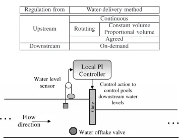
The main goal in canal control for agricultural purposes is to minimize the water waste when supplying water to farmers. Since the offtakes are, in most cases, gravity fed, the requirement of being able to supply water has traditionally been translated into setpoint regulation of water levels [9].

(3)

TABLE II

WATER DISTRIBUTION METHODS(ADAPTED FROM[1])

Regulation from Water-delivery method

Upstream

Continuous Rotating Constant volume

Proportional volume Agreed

Downstream On-demand

Water offtake valve

Control action to control pools downstream water levels Water level sensor Flow direction G at e

…

_…

Local PI Controller

Fig. 4. Local PI controller for downstream water level control (DMPIC).

Further, minimizing the energy consumption to operate the water canal gates should also be a major concern when designing the controller.

There are several methods describing water distribution

in water canals (see Table II). The on-demand method can

be considered truly flexible since in all other cases water offtakes must be known in advance to some extent. Amongst the rigid methods the most flexible one is the agreed method, and for this method the water offtakes are typically fixed with the farmers 24 hr to 48 hr in advance [1]. The number of irrigation canals working with on-demand water delivery methods is however considerably lower compared to rigid methods.

Most of the few automated water canals use DMPIC (Downstream water level Monovariable PI Controller) to

control the pools downstream water levels (see fig. 4).

Similarly, UMPIC (Upstream water level Monovariable PI Controller) is frequently used to control the pools upstream water levels. The main difference between DMPIC and UMPIC relies on the sensor information used to actuate the gates: DMPIC is based on pools downstream water levels, while UMPIC on pools upstream water levels. Since both DMPIC and UMPIC are monovariable, a local single controller is usually applied to each gate. Besides, since there is no information interchanged between each local controller, this type of control configuration is not able to handle disturbance rejection in an efficient way. Interested readers can consult [18] for experimental results of DMPIC and UMPIC on the same experimental irrigation water canal that is considered in this paper.

III. MATHEMATICAL MODEL A. Saint-Venant Equations

The mathematical model of the water canal is based on first principles physical relations. The formulation adopted

in this paper can be easily extended to other canals with similar characteristics. The dynamic behavior of hydraulic systems can be obtained from Reynolds transport theorem and the resulting set of equations are known as Saint-Venant

equations. Equation (1) is called as the continuity equation

and (2) the dynamic equation:

∂Q ∂x + B ∂y ∂t = 0 (1) ∂Q ∂t + ∂ ∂x ! Q2 A " + gA (J − I) + gA∂y ∂x = 0 (2)

where Q is the discharge, y the water level, B the water

surface width, A the water cross-section area, g the gravity

acceleration,x the longitudinal abscissa in the flow direction,

t the time instant, I the bottom slope and J the energy gradient slope that can be accurately approximated by the Gauckler-Manning-Strickler empirical formula [19]:

J = P

4/3

K2_A10/3Q |Q| (3)

whereK is the Gauckler-Manning-Strickler coefficient

(de-termined experimentally) and P is the wetted perimeter.

These equations are nonlinear with unknown analytical so-lution. Thus, the need for linearization and the use of a discretization scheme.

B. Linearization and Discretization: the Preissmann scheme The previously derived Saint-Venant equations are simul-taneously space and time dependent. For their discretization the Preissmann scheme is adopted. Considering the lineariza-tion methodology applied to a point, near to the system steady-state,

Q (x, t) = Qr(x) + δQ (x, t) (4)

y (x, t) = yr(x) + δy (x, t) (5)

where the subscript r stands for steady-state regime and δ

for small increments to this regime. Applying the Preissmann

scheme to the Saint-Venant equations (1)–(2), respectively,

and considering a single pool, results:

a11δQk+1i + a12δyk+1i + a13δQk+1j + a14δyjk+1= = b11δQki + b12δyki + b13δQkj + b14δyjk (6) a21δQk+1_i + a22δyk+1_i + a23δQk+1_j + a24δy_jk+1= = b21δQki + b22δyki + b23δQkj + b24δyjk (7) where: a11= − θ ∆xi a12= # ¯_Bk+1 i $ r 2∆t b11= 1 − θ ∆xi a21= 1 2∆t− 2θ# ¯V_ik+1$_r ∆xi +g # ¯_Ak+1 i φi$_r 4 a22= % V2_Bk+1 i & rθ ∆xi −g # ¯_Ak+1 i $ rθ ∆xi +g # ¯_Ak+1 i ϕi$_r 4 a23= 1 2∆t+ 2θ# ¯Vik+1 $ r ∆xi +g # ¯_Ak+1 i φj$_r 4 a24= % V2_Bk+1 i & rθ ∆xi −g # ¯_Ak+1 i $ rθ ∆xi +g # ¯_Ak+1 i ϕj $ r 4

(4)

b21= 1 2∆t+ 2 (1 − θ)# ¯V_ik+1$_r ∆xi +g # ¯_Ak+1 i φi$_r 4 b22= − % V2_Bk+1 i & r(1 − θ) ∆xi +g # ¯_Ak+1 i $ r(1 − θ) ∆xi +g # ¯_Ak+1 i ϕi$_r 4 b23= 1 2∆t− 2 (1 − θ)# ¯Vik+1 $ r ∆xi +g # ¯_Ak+1 i φj$_r 4 b24= % V2_Bk+1 i & r(1 − θ) ∆xi −g # ¯_Ak+1 i $ r(1 − θ) ∆xi +g # ¯_Ak+1 i ϕj $ r 4 φi= ! ∂J ∂Q " i = 2 P 4/3 K2 sA10/3 |Q| ϕi= ! ∂J ∂y " i =2 3Ji ! 2 P ∂P ∂y − 5 · B A " and a13 = −a11, a14 = a12, b12 = a12, b13 = −b21,

b14 = b12. The indexesi and j refer to contiguous sections

within a pool, whereask refers to time instants; θ ∈ [0; 1] is

the space discretization coefficient. A bar on top of a generic

variable, e.g.s, stands for s (x, t)_ik+1∼= 12

# sk

i + skj

$ , and is related to the time discretization according to the Preissmann scheme.

The linearization and discretization of the water offtakes valves and gates dynamic relations follow a similar

pro-cedure. For offtakes valves considering sections h and j

immediately before and after it, respectively, and assuming

that the approximation δyh= δyj holds, one obtains:

   a11 a21 a12 a22 a13 a23 a14 a24    T    ∂Qk+1_h ∂y_hk+1 ∂Qk+1j ∂y_jk+1    =    a11 a21 a12 a22 a13 a23 a14 a24    T    ∂Qk h ∂yhk ∂Qkj ∂yjk     + -−b11 a11 b21 a21 . -Qkofftake Qk+1_offtake . / 01 2 udisturbance (8)

Notice that in udisturbance the knowledge of Qk+1_offtake is

required. Two situations can occur: either the water offtakes are known in advance or they aren’t, in which case the

approximation Qk+1offtake = Qkofftake is assumed. Finally, the

linearization and discretization of the gates dynamic relations yields:      0 −%∂Qj ∂yi & r 1 −%∂Qj ∂yi & r      T     ∂Qk+1h ∂y_hk+1 ∂Qk+1j ∂y_jk+1    =      0 −%∂Qj ∂yi & r 1 −%∂Qj ∂yi & r      T     ∂Qkh ∂yhk ∂Qk j ∂yjk     + ! ∂f ∂ai " r · ucontrol (9)

where variable a represents the gates aperture. Notice

that the partial derivatives depend on the considered gate characteristics and type, which can be normally written

as Q = f (yi, yj, a), with Q being the flow crossing the

gate section, yi andyj the water levels immediately before

and after the gate, respectively. For sluice gates, Q =

cv #

B0a + ma2

$ 3

2g (yi− yj), while for overshot gates,

Q = cvl√2g (yi− a)3/2 whereB0 is the pool base width,l

M P C

…

_…

QP Optimization C an al

Water level data;

Water offtake data. Gates aperture; Water inflow.

Internal model

! Cost function ! Constraints

Fig. 5. MPC of a water canal.

is the gate top width andcv is a correctional experimentally

determined coefficient.

The mathematical model description in a state space format is finally obtained by gathering all the previous linearized and discretized hydraulic equations [20]:

xk+1= Adxk+ Bdudk+ Bcuck (10a)

yk = Cxk (10b)

where uc and ud contain all the manipulated variables

ucontrol and udisturbance, respectively. The final number of

states will depend on the number of sections considered in the discretization.

IV. MODEL PREDICTIVE CONTROLLER The application of MPC to hydraulic systems has great po-tential. Besides being an optimization-based controller where physical constraints can be easily integrated, it can cope with both known and unknown in advance water offtakes,

while handling the multivariable nature of the model. Fig.5

presents a schematic configuration of the MPC applied to a water canal.

Implicit to any predictive control algorithm is the opti-mization of a cost function, normally subjected to constraints.

In this paper the selected cost function,J, takes the following

form: J(k) = Hp 4 i=Ha 5 5 5ˆyk+i|k− ry k+i55 5 2 Qi+ Hc−1 4 i=0 5 5 5ˆuck+i|k− r k+i uc 5 5 5 2 Wi + Hc−1 4 i=0 5 5 5∆ˆuck+i|k 5 5 5 2 Ri (11)

where ˆyk+i|k are the predicted outputs for instant k + i

calculated at time instant k, and ryk+i their correspondent

references; ˆuck+i|k are the optimal control inputs for instant

k+i calculated at time instant k, and rk+iuc their correspondent

references; ∆ˆuck+i|k are the control inputs changes. Hp is

the prediction horizon and Hc is the control horizon. The

parameterHa is specially useful when dealing with systems

with time delay (in this case,Ha= 1). The first term of the

cost function weights the tracking error, the second term the deviations of the control action from the desired reference

(5)

TABLE III

STEADY-STATE WATER LEVELS

Pool/Section Upstream Middle Downstream Pool 1 544 (mm) 572 (mm) 600 (mm) Pool 2 559 (mm) 579 (mm) 600 (mm) Pool 3 541 (mm) 57 (mm) 600 (mm) Pool 4 595 (mm) 597 (mm) 600 (mm)

whereas the third term weights the “energetic cost” of the

control input.Qi,Wi andRi are positive-definite weighting

matrices.

Several types of constraints must be taken into considera-tion when dealing with water canals. These are due, in most cases, to water level and actuators constraints. The dynamic relations of water level constraints can be obtained from the canal cross section height and the water level at steady-state regime in each section. By taking the Saint-Venant dynamic

equation (2) assuming constant nominal flow and water level,

one obtains: ∂yr ∂x = I − J 1 −Vr2Br gAr (12)

where Vr ≡ Q_Ar_r. This non-linear first order differential

equation is known as the backwater curve. Its linearization and discretization, for the experimental water canal assuming

a steady-state regime (Qr = 30L/s) and considering the

boundary conditions (y = 600 mm) downstream of each pool, gives the steady-state water level distribution in all

sections, presented in table III. The water level constraints

can be easily obtained from the height of the canal pools and the fact that water levels cannot take negative values.

Constraints related to the input changes and additional, more restrictive constraints on the water level can also be considered.

V. EXPERIMENTAL RESULTS

The experimental results obtained with MPC are com-pared with the DMPIC and UMPIC (also implemented). The control algorithms were developed using Matlab, and an interface between Matlab and the supervising SCADA system makes use of a proprietary software package designed specifically for the communication between both systems. This software is based on the DDE protocol and enables the development of any type of controller in Matlab without any previous knowledge of the SCADA or the PLC network responsible for the local canal control. It can also be used to exactly reproduce water offtakes schedules without any human intervention.

The active sets QP optimization algorithm was adopted for the implementation of the predictive controller using the Model Predictive Toolbox from Matlab [21]. To evaluate the controllers performance several performance indicators are available [22]. In this paper the following well known performance indicators are used:

• Integrated absolute error: IAE =6 |y − ry|;

• Maximum absolute error: MAE =max |y − ry|;

• Integrated gate movement: IAW =6 |∆a|;

• Maximum gate aperture: MAW =max |a − ra|;

where ra is the gate nominal aperture. The first two

indi-cators refer to water levels, while the last two refer to the gate movements. High water level deviations and great gate movements should be avoided in any water canal [23]. To this view, the following performance index is also monitored:

β = n 4 i=1 7 T 0 - |yi− ryi| 16.5 + |∆ai| . dt = IAE 16.5 + IAW (13)

where T is the total test time, yi is the controlled water

level in pool i with reference ryi,∆ai is the gate aperture

variation in pooli, and n is the total number of pools. The

value16.5 is used to balance both terms in the index. This

index is particularly useful since it gives a general evaluation of each of the controllers performance.

A. Upstream water level control

The performance of MPC and the UMPIC are compared when controlling the pools upstream water levels. The results

obtained for a water offtake of 10L_/_s _{extracted from the}

3rd offtake valve of the canal during the time intervalt =

[200 s; 400 s] are presented in fig. 6 and in table IV (The

notation S#T# indicates sensor S# in pool T#, thus S1T2 refers to the upstream water level measured by sensor 1 in pool 2. Likewise, the notation G# is used to indicate gate number #). 0 200 400 600 800 −30 −25 −20 −15 −10 −5 0 5 10 15 Time (s) D ev ia ti o n (mm )

Water Level Deviation in Section S1T2

0 200 400 600 800 −30 −25 −20 −15 −10 −5 0 5 10 15 Time (s) D ev ia ti o n (mm )

0 200 400 600 800 −15 −10 −5 0 5 10 15 20 25 30 Time (s) D ev ia ti o n (mm )

0 200 400 600 800 −15 −10 −5 0 5 10 15 Time (s) D ev ia ti o n (mm )

Fig. 6. Pools upstream water level control results (First column: MPC; second column: UMPIC; Rows: upstream water levels in pools 2, 3, and 4, respectively).

(6)

TABLE IV

UPSTREAM WATER LEVEL CONTROL—PERFORMANCE INDICATORS

IAE (mm) MAE (mm) S1T2 MPC 2590 14 UMPIC 7172 26 S1T3 MPC 2361 14 UMPIC 5733 26 S1T4 MPC 1948 8 UMPIC 3563 14 IAW (mm) MAW (mm) G1 _UMPICMPC 545₃₇₂ 206₇₀ G2 _UMPICMPC 268₁₈₁ 84₅₃ G3 _UMPICMPC 176₈₀ 32₂₃ β MPC 1408 UMPIC 1632

The high oscillation of the water level deviations captured by the sensors is caused by the fact that these sensors are located near the gates. The water that flows under the gates produces disturbance waves that are captured by these sensors. Comparing the evolutions it can be concluded that MPC has a better performance leading to smaller water level deviations than the UMPIC controller (cf. performance

indicator IAE in table IV). Furthermore, the performance

index,β, is smaller for the MPC than it is for the UMPIC

controller which is a clear indication that MPC outperforms the UMPIC.

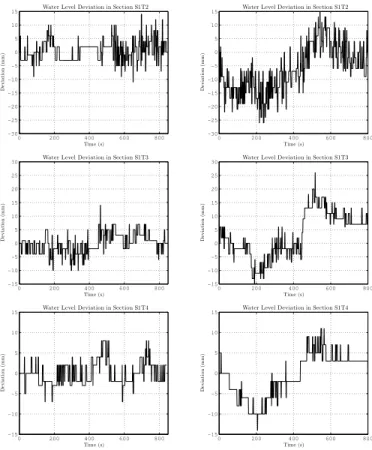
B. Gate malfunctioning

The performance of MPC and of the DMPIC is compared under the scenario of a gate malfunctioning. This experiment is also useful to show the advantage of considering a multi-variable controller instead of a monomulti-variable one. Whereas monovariable controllers divide the system into distinct parts without regarding its interconnections, multivariable controllers make use of cross information along the canal sensors to produce the best control action. This experiment was conducted considering the 3rd gate fixed at its nominal

position, with a water offtake of 10L_/_s_{in the 3rd offtake valve}

between time instants t = 150 s and t = 415 s. The results

obtained with both controllers are presented in figure7 and

tableV.

Both controllers experienced difficulties in minimizing the water level deviations. However MPC produces better results than the DMPIC. For instance, notice how MPC is able to take the water level deviation in section S3T3 to zero during the water offtake even with the gate G3 fixed. The MPC is able to keep the water level deviations smaller while making approximately the same use of the gates as the DMPIC

controller (see indicators IAE and IAW from tableV).

C. Severe water offtakes

The performance of MPC is compared with the DMPIC when severe water offtakes are considered. In this experi-ment, rapidly varying water offtakes that reach up to 83% of the nominal flow were extracted from the canal offtakes

0 100 200 300 400 500 600 −15 −10 −5 0 5 10 15 Time (s) D ev ia ti o n (mm )

0 100 200 300 400 500 600 −10 −5 0 5 10 15 Time (s) D ev ia ti o n (mm )

Fig. 7. Gate malfunctioning results (First column: MPC; second column: DMPIC; Rows: upstream water levels in pools 1, 2, and 3, respectively).

TABLE V

GATE MALFUNCTIONING—PERFORMANCE INDICATORS

IAE (mm) MAE (mm) S3T1 MPC 3134 11 DMPIC 4076 14 S3T2 MPC 2469 9 DMPIC 3826 15 S3T3 MPC 4745 16 DMPIC 8978 28 IAW (mm) MAW (mm) G1 _DMPICMPC 163₁₅₀ 60₇₃ G2 _DMPICMPC 157₁₃₉ 69₇₆ G3 _DMPICMPC 0₀ 0₀ β MPC 948 DMPIC 1313

valves following the profile given in fig. 8. The results

obtained with MPC and with the DMPIC are depicted in

fig. 9 and the corresponding performance indicators are

presented in tableVI.

The MPC is able to keep the water level deviations in a smaller range than the DMPIC (cf. performance indicator MAE), at the expense of a slight increase in gate usage (cf. performance indicator IAW). Even though the difference in gate usage between DMPIC and MPC is small, this has a negative effect on the overall performance of the DMPIC. A maximum water level deviation of 28mm was measured

(7)

0 500 1000 1500 0 2 4 6 8 10 12 Time (s) L / s Water Offtakes

Offtake 1 Offtake 2 Offtake 3

Fig. 8. Water offtakes profile.

0 500 1000 1500 −20 −15 −10 −5 0 5 10 15 20 25 Time (s) D ev ia ti o n (mm )

Water level Deviation in Section S3T1

0 500 1000 1500 −30 −20 −10 0 10 20 30 Time (s) D ev ia ti o n (mm )

Fig. 9. Severe water offtakes results (First column: MPC; second column: DMPIC; Rows: upstream water levels in pools 1, 2, and 3, respectively).

for DMPIC, compared to 12mm that was registered for the MPC.

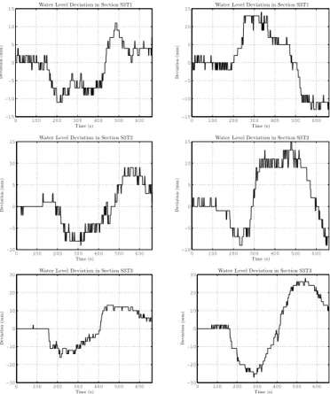
D. Water level setpoint tracking

The problem of water level setpoint tracking change through time is here analyzed. This type of disturbance is more likely to occur on rigid water distribution methods than on flexible ones. For example the water levels setpoint can change to higher values during Summer time, due to the increase in water usage, while it can be reduced to lower values during Winter season. The simulation of this real situation is made considering a staircase-like change on the reference of the 3rd downstream water level. The

TABLE VI

SEVERE WATER OFFTAKES—PERFORMANCE INDICATORS

IAE (mm) MAE (mm) S3T1 MPC 6612 13 DMPIC 11147 22 S3T2 MPC 5067 13 DMPIC 14691 23 S3T3 MPC 5636 12 DMPIC 16032 28 IAW (mm) MAW (mm) G1 _DMPICMPC 868₅₀₆ 87₉₇ G2 _DMPICMPC 767₆₁₅ 66₉₄ G3 _DMPICMPC 1170₇₁₅ 170₁₈₁ β MPC 3855 DMPIC 4374 0 50 100 150 200 250 300 350 −10 0 10 20 30 40 50 60 Time (s) D ev ia ti o n (mm )

Water level measured Water level reference

Fig. 10. Water level setpoint traking

experimental results for the MPC are shown in fig. 10.

The performance indicators for the MPC as well as for the

DMPIC are presented in tableVII. This test clearly shows

that MPC is better than the DMPIC since it is able to closely follow the water level reference. Notably the MPC is able to make slightly less use of the system gates (smaller IAW) while keeping water levels deviations (IAE) smaller than the DMPIC.

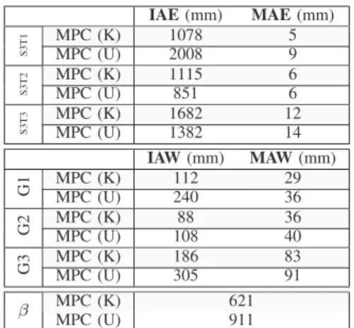
E. known in advance water offtakes

The MPC performance is tested in the situation when

water offtakes are available in advance. TableVIIIpresents

the performance indicators for this case study. These indi-cators clearly show that when the water offtakes are known

TABLE VII

WATER LEVEL SETPOINT TRACKING—PERFORMANCE INDICATORS

IAE (mm) MAE (mm) S3T3 MPC 930 9 DMPIC 3591 21 IAW (mm) MAW (mm) G3 _DMPICMPC 246₂₅₆ 125₈₈ β MPC 1303 DMPIC 1991

(8)

TABLE VIII

WATER OFFTKES KNOWN(K)AND UNKNWON(U)IN ADVANCE—

PERFORMANCE INDICATORS IAE (mm) MAE (mm) S3T1 MPC (K) 1078 5 MPC (U) 2008 9 S3T2 MPC (K) 1115 6 MPC (U) 851 6 S3T3 MPC (K) 1682 12 MPC (U) 1382 14 IAW (mm) MAW (mm) G1 MPC (K)_{MPC (U)} 112₂₄₀ 29₃₆ G2 MPC (K)_{MPC (U)} ₁₀₈88 36₄₀ G3 MPC (K)_{MPC (U)} 186₃₀₅ 83₉₁ β MPC (K) 621 MPC (U) 911

in advance the MPC is able to benefit from this additional knowledge improving its performance. Notice that although the IAE indicator is approximately the same, the IAW (related to the gates movements) is much smaller when the water offtakes are known in advance. This is mainly due to the preventive response of the MPC: previously to a water offtake it starts closing the gates thus increasing the resident volume of water to better face the future water offtake.

VI. CONCLUSIONS

This paper presented the first experimental results of a MPC applied to the water canal located at the University of

´

Evora, Portugal. A wide range of real-life typical situations were covered in the experiments showing the effectiveness of the control approach over other classical water canal control strategies, namely two monovariable PI controllers. The MPC was able to handle water offtakes (whether known or not known in advance), water level reference tracking and process failure, while obeying the canal constraints.

The dynamic model of the water canal was obtained based on the Saint-Venant equations, which proved to be suitable for being integrated in the predictive controller. Besides, authors believe that this control setup can be extended to other similar water distribution networks since the model used is mostly based on canal geometric characteristics.

ACKNOWLEDGMENTS

This work is partially supported by projects

POCI/EME/59522/2004, PTDC/EME-CRO/69117/2006,

and co-sponsored by FEDER, Programa Operacional

Ciência e Inovação 2010, FCT, Portugal. REFERENCES

[1] J. R. Raposo,A Rega: dos primitivos regadios às modernas técnicas de rega, 1st ed. Fundação Calouste Gulbenkian, Nov. 1996.

[2] J.-P. Baume, P.-O. Malaterre, and J. Sau, “Tuning of PI controllers for an irrigation canal using optimization tools,” inProceedings of the USCID Workshop, A. C. . S. Anderson, Ed., Phoenix, USA, 1999, pp. 483–500.

[3] I. Guenova, X. Litrico, , and D. Georges, “Modelling and robust PID control of an irrigation canal pool,” inProceedings, Modelling, Identification and Control, Spain, 2004.

[4] X. Litrico, V. Fromion, J. Baume, and M. Rijo, “Modelling and PI controller design for an irrigation canal,” in European Control Conference, Cambridge, UK, 2003.

[5] C. Seatzu, “Robust PI decentralized control law for open channel hydraulics systems,” in Proceedings European Control Conference, Karlsruhe, Germany, 1999.

[6] D. C. Rogers, D. G. Ehler, H. T. Falvey, E. A. Serfozo, P. Voorheis, R. P. Johansen, R. M. Arrington, and L. J. Rossi, Canal Systems Automation Manual, Bureau of Reclamation, Denver, Colorado, USA, 1995.

[7] P. O. Malaterre, “Pilote: Linear quadratic optimal controller for irrigation canals,”ASCE Journal of Irrigation and Drainage, vol. 124, no. 4, pp. 187–194, 1998.

[8] A. Garcia and J. J. DeVries, “Open channel transient flow control by discrete time LQR methods,”Automatica, vol. 28, no. 2, pp. 255–264, 1992.

[9] E. Weyer, “LQ control of an irrigation channel,” inProceedings of the 42nd IEEE Conference on Decision and Control, Maui, Hawaii, USA, Dez. 2003, pp. 750–755.

[10] C. Garcia, D. M. Prett, and M. Morari, “Model predictive control: theory and practice — a survey,”Automatica, vol. 25, no. 3, pp. 335– 348, May 1989.

[11] J. M. Maciejowski, Predictive Control with Constraints, 2nd ed. Prentice-Hall, May 2001.

[12] J. C. Pag`es, J. M. Compas, and J. Sau, “MIMO predictive control with constraints by using embedded model-based systems,” IEEE International Conference on Systems, Man, and Cybernetics, vol. 4, pp. 3902–3907, 1998.

[13] V. M. Rutz, C. Ruiz, and L. Ramirez, “Predictive control in irrigation canal operation,”IEEE International Conference on Systems, Man, and Cybernetics, vol. 4, pp. 3897–3901, 1998.

[14] J. Rodellar, M. Gomes, and L. Bonet, “Control method for on-demand operation of open-channel flow,”Journal of Irrigation and Drainage Engineering, vol. 119, no. 2, pp. 225–241, 1993.

[15] P.-O. Malaterre and J.-P. Baume, “Modeling and regulation of irri-gation canals: existing applications and ongoing researches,” IEEE International Conference on Systems, Man, and Cybernetics, vol. 124, no. 4, pp. 3850–3855, Oct. 1998.

[16] A. J. C. B. Saint-Venant, “Théorie du mouvement non-permanent des eaux, avec application aux crues des rivières et à l’introduction des marées dans leur lit,”Acadmie Scientific Paris, vol. 73, pp. 148–154, 237–240, 1871.

[17] J. A. Mantec´on, M. G´omez, and J. Rodellar, “A simulation-based scheme for simulation of irrigation canal control systems,”Simulation, The Society for Modeling and Simulation International, vol. 78, no. 8, pp. 485–493, Aug. 2002.

[18] M. Rijo, “Local automatic control modes in an experimental irrigation canal,”Irrigation and Drainage Systems, vol. 17, no. 3, pp. 179–193, Aug. 2003.

[19] A. de Carvalho Quintela, Hidráulica, 9th ed. Fundação Calouste Gulbenkian, May 2005.

[20] O. S. Balogun, M. Hubbard, and J. J. DeVries, “Automatic control of canal flow using linear quadratic regulator theory,” Journal of Hydraulic Engineering, vol. 114, no. 1, pp. 75–102, Jan. 1988.

[21] A. Bemporad, M. Morari, and N. L. Ricker,Model Predictive Control Toolbox for use with MATLAB, 2nd ed., The MathWorks, Mar. 2005.

[22] M. Bos, “Performance indicators for irrigation and drainage,” Irriga-tion and Drainage Systems, vol. 11, no. 2, pp. 119–137, 1997.

[23] M. Rijo, J. Honrado, C. Arranja, and M. Almeida, “Controlo de um canal de rega. parte ii: Calibração hidráulica,” 2006.