UNIVERSIDADE DE ÉVORA
DEPARTAMENTO DE ECONOMIA
DOCUMENTO DE TRABALHO Nº 2006/07
March
On the Demand of Environmental Goods with Intertemporally Dependent
Preferences
José Manuel Madeira Belbute*
Universidade de Évora, Departamento de Economia
Paulo Brito**
Technical University of Lisbon – Instituto Superior de Economia e Gestão
*
Associtate Professor -University of Évora, Department of Economics ([email protected]) **Technical University of Lisbon – Instituto Superior de Economia e Gestão ([email protected])
UNIVERSIDADE DE ÉVORA
DEPARTAMENTO DE ECONOMIA
Largo dos Colegiais, 2 – 7000-803 Évora – Portugal Tel.: +351 266 740 894 Fax: +351 266 742 494
Resumo/Abstract:
In this paper, we use a simple framework to analyze two issues relating the canonical model of environmental economics. The first is related with the consistency between the intertemporal and the instantaneous structure of the utility function. The second is related with to the specific stability and dynamic properties of the model and to its response to relative price and income exogenous changes. We find that, if there is bounded adjacent complementarity in demand for environmental goods, intertemporal independence in the demand for the other goods and if the utility function displays goods separability, then there will be short-run complementarity between the stock of tastes and the financial wealth. Increases in income will rise the long-run demand for environmental good while increases in the relative price will decrease it.
Palavras-chave/Keyword:
Classificação JEL/JEL Classification: Consumer behavior, intertemporal dependent preferences, environmental economics
1. Introduction
One of the most used assumption in intertemporal allocation problems is intertemporal independence. When one use an objective function as
∫
∞U e−δtdt0 (.) we are explicitly
assuming the altruistic component of the problem but also that that preferences are intertemporal independent. In other words, the rate at which consumer will substitute consumption in time t for consumption in time t+1 is, at the margin, independent from the amount he/she has consumed in t-1 and/or of the amount he expects to consume in
t+2.
Environmental goods and services (or “environmental quality” as it is often used) have specific attributes which differentiate them from other private or conventional public goods and services. Whether it is a “bad” (pollution) or a positive good, environmental goods and services are public goods that are endowed by individuals rather then purchased (they are said to be non-rival and non-excludable). And although national parks, beautiful landscapes, clean air, sea level, species diversity, the effect of ozone layer, etc, do not have a market in which one can observe behaviors that are related to environmental quality, it is often possible to measure people’s willingness to pay to secure a benefit (or the willingness to accept compensation to forgo the same benefit) from environmental goods by using data from those markets.
Two main features should be emphasized as regard to the demand of these goods. First, given the present civilizational and cultural pattern of preferences, consumers have to endure a learning-by-consuming (or an habit-formation) process to full enjoy (and use) them and to undertake a "green- economic behavior". This “learning-by consuming” process is assumed to be equivalent to “adjacent complementarity” (see Ryder and Heal (1973 and also Becker and Murphy (1988)) and, differently to what is commonly assumed in the literature of habit formation3, the “stock of environmental quality” is
assumed to be a beneficial addiction; it has a positive value for the consumer.
The second feature is that the environmental goods and services may be assumed to be pure consumer goods. The most exclusive outcome from their “consumption” is an increase in utility, related to various form of aesthetic fruition. Our hypothesis is that utility enhancement motive is dominant and the consumers do not expect any future increase in income by devoting time and resources to environmental fruition.
Of course, the stock of environmental assets could be seen as an instantaneous source of present income and, if so, the process of cultivation of taste could be seen as an equivalent to any other educational activity. In this context, the dynamic model for environmental demand would be a mere extension of the simplest model of endogenous growth literature of Lucas (1988) or Uzawa (1965). Consider
Though one could easily find relations between the two perspectives, our assumption considers that the utility enhancement motive is dominant and therefore the consumers do not expect any future increase in income by devoting time and resources to environmental fruition. In this sense, the stock of environmental taste is distinct from human capital and the canonical model of environmental economics is different from one in the endogenous growth literature.
In order to address the effects of changes in relative prices, we will need to consider an economy with two composite goods; environmental and non-environmental goods. At the best of our knowledge, the literature on the demand for environmental quality has
addressed the issue of intertemporally dependent preferences even in the presence of one-good economy.
Habit-formation models for two-good economies have already been used within a international macroeconomic framework (see Mansoorian (1993) and Mansoorian (1998)) but the focus of these approaches were not the structure of the intertemporal preferences. Moreover, the usual assumption about distant complementarity used in these studies contradicts the correspondence between adjacent complementarity and learning-by-consuming as well as the specificity of environmental goods.
To summarize, this paper addresses two major issues of the demand of environmental quality that need further investigation as well empiric validity: the determination of a coherent set of assumptions, regarding the structure of preferences, and the study of the stability and comparative dynamics of the equilibrium. Given the well known technical complexity involved, we will use the simplest framework to fix ideas: we consider a two-good economy where environmental two-good is subject to a cultivation of taste process and a non-environmental good whose demand displays both own and crossed intertemporal independence. Income is assumed to be an exogenously given endowment. We abstract from economic growth and from distortions induced by public authorities. Agents are assumed to be homogenous.
The paper is organized as follows: section 2 presents the model, section 3 extends Ryder & Heal (1973)'s definitions of adjacent and distant complementarity for a two-goods economy, section 4 studies the dynamics, section 5 presents the dynamic response of the demand for both environmental and non-environmental goods after a non-anticipated and permanent increases in exogenous income and in the relative price of environmental good and section 6 concludes the paper.
2. The model
The model we are going to develop involve both an extension and a specialization of the standard habit- formation model. The extension involves a two-good framework and it is needed in order to analyze changes in relative prices. Additionally we assume that preferences relating non-environmental good are not intertemporally dependent in order to emphasize only the distinct features of environmental goods.
Formally, we assume that the representative household derives utility not only from current consumption from all sort of goods but also he enjoys being "environmentally educated ". His problem is to optimally choose the trajectory of consumption of environmental and non-environmental goods, a(t) and c(t), by maximizing the inter temporal utility function
[
]
∫
∞ −0 uc(t),a(t),k(t)e dt t
δ (1)
where δ > 0 is the time rate preference and k(t) being the stock of environmental taste at moment t, which is given by
∫
− − − + =k e t t a e t d t k 0 ) ( 0 ( ) ) ( ρ ρ τ ρ τ τ (2) were we assume that the rate of learning-by-consuming is equal to the rate of depreciation of the stock of tastes, ρ. Instantaneous utility u(c,a,k) exhibits the following properties; uc >0, ua >0, uk >0 which contrasts with Ryder & Heal (1973) assumptionthat uk <0. Finally, the remaining assumptions are related to both the intertemporal and intratemporal curvature and separability properties of utility. Namely, it is assumed that learning-by-consuming is equivalent to own adjacent complementary as in Ryder & Heal (1973). The consumption of non-environmental goods displays both own and crossed intertemporal independence. At last, we assume that instantaneous utility is concave in (c, a, k ) and, to simplify the model, that is separable4.
Finally, the consumer is constrained by the financial budget constrain
[
]
( )∫
− − − + =bert t w c a ert d t b 0 0 ( ) ( ) ) ( τ π τ τ τ (3) where w is the exogenous income and π is the relative price of the environmental good as regard to non-environmental goods.3. The structure of intertemporal preferences
This section extends Ryder & Heal (1973)'s definitions of adjacent and distant complementarity for a two-goods economy by defining own and crossed complementarities. Next, we will formally state the assumptions characterizing the canonical environmental-economics model and we will prove that only environmental/non-environmental separability is compatible with the sufficient conditions for an optimum.
3.1 Intertemporal complementarities
Take t as the initial time. Then, equation (1) defines a value funtional 0
( )
∫
∞ − −∫
− − − + = 0 0 0) ( ) ( 0 0 t ( ), ( ), ( ) t t t t t t a e d e dt e k t a t c u t V ρ ρ τ ρ τ τ δ . (4) Let{ }
c(t)+∞t0 and{ }
a(t)t+∞0 be given trajectories for the consumption of non-environmental and environmental goods, respectivelly. The first-order Volterra derivative measures the marginal change in the value of the functional after an unit instantaneous increase in the value of one trajectory at t=t1>t0[]
∫
∞ −( + )[]
− + = 1 1 1 . . ) (1 t k t t a t a t e u e e u dt V δ ρ ρ ρ δ (5)[]
. ) ( 1 1 t c ct e u V = −δ (6) and the marginal rates of substitution between trajectories displaying changes at t and 11 2 2:t t t > are = ) ( ) ( ) , ( 2 1 2 1 t VV tt t R a a a and = ) ( ) ( ) , ( 2 1 2 1 t VV tt t R c c
c for the consumption of
environmental and non-environmental goods, respectively.
Intertemporal dependency is measured by change in the marginal rates of substitution between the trajectories of consumption changing at t and 1 t for shifts in the 2
trajectories at t3:t3 >t2 >t1,
4 However, though it may be separable across stock/flow or non-environmental/environmental dimensions, the latter is consistent with the other assumptions.
[
]
2 2 3 2 1 3 1 2 3 2 1 ) ( ) , ( ) ( ) , ( ) ( ) ; , ( t V t t V t V t t V t V t t t R i ij i ij i ij − = (7) Its signs are interpreted as follows: if Rij(.)< 0 we say that there is own (crossed) adjacent complementarity, if i=j(i≠ j); if Rij(.)= 0 we say that there is own (crossed) intertemporal independence, if i= j(i≠ j); and, finally, if Rij(.)> 0 we say that there is own (crossed) distant complementarity, if i= j(i≠ j).To specify those definitions further we need to determine the second-order Volterra derivatives which give the change in the first-order Volterra derivative of i at t when 1
there is a unit change in j at t . Let 2 Vij(t1,t2), for i,j=a,c, denotes that derivatives.
Then ( + ) +
(
)
( + )∫
∞ −( + )(
)
− + = 2 2 1 1 2 ( ,... ( ),... ( ) ) , ( 2 2 2 2 1 t t ka t t t t kk aa t t e u at e e u ct kt dt V ρ δ ρ ρ ρ ρ δ ρ (8) ( )(
( ),...)
) , (t1 t2 e 2 1 u ct2 Vac = −ρ+δt +ρt ρ kc (9) 0 ) , ( ) , (t1 t2 =V t1 t2 = Vca cc (10) If we locally evaluate the derivatives of the marginal rates of substitution along a constant path such that a(t) = k(t) for all t, then we get ∆ + + + + = k a kk ka aa u u u u t t t R δ ρ ρ δ ρ ρ ρ 2 ) ; , (1 2 3 , ∆ + + = k a kc ac u u u t t t R δ ρ ρ ρ ) ; , (1 2 3 and Rca(t1,t2;t3)=Rcc(t1,t2;t3)=0 where (t2 t1) (
[
e )(t1 t3) e( )(t21 t3)]
e − + − − + − =∆ δ ρ δ ρ δ < 0 as t3 >t2>t1, if we ignore tha argumentas in the
derivatives o u(.).
Now we can supply an intuition for the signs of R . Ther is own adjacente (distant) ij
complementarity in consumption of the environmental good if Raa(.) is negative
(positive). This means that if there is a unit increase in a(t3) the marginal rate of substitution Ra(.) reduces (increases). That is, consumption shifts from a(t1) to a(t2). There is crossed adjacente (distant) complementarity between a unit change in c(t3) and the trajectory of consumption of environmental good if Rac(.) is negative (positive). This means that if tere is a unit increase in c(t3) the the marginal rate of substitution Ra(.) reduces (increases) and consumption sifts from a(t1) to a(t2). As Rcj(.)= 0, for
c a
j= , , then the rate of marginal substitution of the non-environmental good is independent from future changes in both goods and, equivalently, preferences are intertemporally additive as far as c is concerned.
Formally, we assume the following:
Assumption 1: Beneficial properties: ua >0, uc >0 and uk>0
Assumption 2 :Bounded own adjacent complementarity in consumption of the environmental
0<uka +2ρρ+δ ukk<−2ρρ+δ uaa
Assumption 3: Crossed intertemporal independence in the consumption of the environmental
good as regard the non-environmental good: ukc =0 Assumption 4: u(.) is concave in (a,c,k).
3.2 Intertemporal complementarities and intratemporal
separabilities
Next, we would like to simplify the problem by introducing weak separability in the instantaneous utility function. However, we would like to do it in such a way that the following holds:
Assumption 5: u(c,a,k) is consistently instantaneously separable.
There are two obvious candidates. First, there is stock-flow separability if u=u
[
µ( )
a,c,k]
, where µ(.) and k are weakly separable, that is =0 ∂ ∂ ∂ ∂ ∂ ∂ c u a u k . Additionally, assume
that (.)µ is strictly increasing, linearly homogeneous and strictly quasi-concave in both arguments. This assumption is typically done in macro models involving habit-formation because it allows for both a simplification of the problem and a simpler treatment of the relative prices. As the function µ(.) is a static indirect utility function, standard duality results imply that u(.) would be a function of an index of total consumption and the stock of habits. In this case, a static true cost of living index could be built and total consumption expenditure would separate between total price and quantity indices.
Second, there is environmental versus non-environmental separability if u=u
[
η( )
a,k,c]
, where η(.) and c are weakly separable, that is =0 ∂ ∂ ∂ ∂ ∂ ∂ k u a u
c . Assume also that η(.) is
strictly increasing in both arguments, not linearly homogeneous (it could be additively separable) and concave.
Lemma 1: Let assumptions1 to 5 holds. Then u(c,a,k) is weakly separable into
environmental/non-environmental goods, i. e. u=u
[
η( )
a,k,c]
.Proof. Let there be stock-flow (weak) separability, that is u=u
[
µ( )
a,c,k]
. Thena a u u = µµ , uc=uµµc, uaa =uµµµa2+uµµaa, uac =uca =uµµµaµc+uµµac, ucc =uµµµc2+uµµcc, a k ka ak u u u = = µ µ and uck =ukc=uµkµc.
As uck =ukc =0 then uµk =0 because µa>0. This also implies that uak =uka =0 and that there will only exist own adjacent complementarity if u(.) is convex as regard to k, that is ukk>0. From the concavity of u(.) as regard µ (uµµ <0), the strictly quasi-concave property of µ(.) (that is = 2 + 2 −2 <0 ac c a aa c cc a U µ µ µ µ µ µµ ) and as u( )a,c =uµuµµU and ( ) u u u U
ua,c,k = µ µµ kk , then we have sign u ( )a ,c = −sign u µµ= −sign u u
(
µµ kk)
=sign u (a ,c ,k) .Therefore, the Hamiltonian is not concave as regards to (a,c,k) and the Mangasarian sufficient conditions for a maximum does not hold (see Kamien and Schwartz (1991), p. 221).
Now, consider the environmental/non-environmental weak separability, that is
( )
[
a k c]
u u= η , , . Then ua =uηηa, uk =uηηk, uaa =uηηηa2+uηηaa, uak =uka =uηηηaηk+uηηak, kk k kk u u u = ηηη2+ ηη , a c ca ac u uu = = ηη and uck=ukc =uηcηk. Intertemporal independence in
consumption of non-environmental goods holds if and only if uηc =0, as we have ηk >0. In this case, both own adjacent complementarity as regard the environmental good
( 0 2 2 2 > + + + + + = + + kk k a k ak kk ka u u u u η δ ρ ρ η η δ ρ ρ η η δ ρ ρ η
ηη ) and the concavity conditions
(uηη≤0,ηkk <0) will hold, if ηak is positive and sufficiently large in absolute value. If,
additionally, ηaa <0, ucc <0 and η(.) is both concave and quasi-concave, then sufficient conditions for a maximum, according to Mangasarian' theorem, also holds:
0 < aa u , ( )=
(
2+)
>0 aa a cc ac u u u u ηηη ηη and u( )ack =uηucc[
uηη(
ηa2ηkk−2ηkηaηka+ηk2ηaa) (
+uηηaaηkk−ηak2)
]
<0.Corollary 1: If there is stock-flow weak separability, then the second order derivatives of the
utility function verify: uaa <0, ucc <0, ukk<0, uak>0 and uac=ukc=0.
4. The dynamical properties of the model
The intertemporal optimization problem for the representative consumer defines the indirect utility function
[
]
∫
∞(
)
− = 0 , , , max ) 0 ( ), 0 ( k ua c ke dt b U t c a δ (11)where u(.) verifies assumptions 1 to 5, subject to the stock-flow relation for environmental goods in its differential form, k•=ρ
(
a−k)
, and to the instantaneous and intertemporal budget constrain, b• =w−c−πa+rb, for k(0) and b(0) given.From the maximum principle of Pontryiagin, the optimal levels for consumption,
( )
a )), cwill verify π ρ b k a a ck p p u ( , , )+ = (12) b c ac k p u ( , , )= (13) where p and k p are the co-state variables associated to the sock of taste and b
financial wealth, respectively. For each good, the consumer derives optimal strategies by equating the marginal benefits from consumption, (witch are equal to the direct marginal utility plus the value of the marginal update in taste for the case of environmental good) to marginal costs (measured by the value of the change in foregone savings:
(
p ,p ,k,π)
aa) = ) k b , a)pk >0, a)pb <0, a)k>0, a)π <0 and c) =c)
( )
pb with c)pb <0).The optimal level for the consumption of environmental goods is an increasing function of both the level and the dual value of taste and it is a decreasing function of the dual value of financial wealth and of the relative price. The first effect captures the inertial feature of the stock of taste over the current flow of consumption. The second and third effects involve intertemporal choices: there is (intertemporal) complementarity as regards choices between the flow and the stock of taste and substitutability between present and future consumption, for a given level of the resources. The last is an instantaneous income effect: the rise in one price decreases the real level of resources available for consumption. As far as the non-environmental good is concerned, there is
only a intertemporal effect related to the substitutability between present and future consumption, for a given level of the resources.
The optimal solution will involve through time according to the following system of non-linear canonical equations
(
)
p u(
ac k)
p•k= δ +ρ k− k ) ,,) ) (15)(
)
b b r p p• = δ − (16)(
a k)
k•=ρ )− (17) rb a c w b• = −)−π)+ (18) for k(0) and b(0) given and for bounded state variables. The first two equations can be interpreted as stating optimal arbitrage relations for the two stocks: (i) the marginal utility of the stock of taste plus the increase in its value should equal the sum of the rate of time preference (the price of postponing consumption) with the rate of depreciation of tastes; (ii) The total income extracted from holding financial assets (interests plus capital gains) should equal the rate of time preference.The intertemporal budget constraint is equivalent to assuming that financial wealth is bounded and that the representative household is kept as a small economic unit. This implies that the stady-state of time preference rate should be equal to the real interest rate,
δ = r (19)
and that the stady-state
(
pk,pb,a,c,k,b)
exists, through it is not unique. It is caracterized by the fllowing equations: first, the marginal utility of taste is equal to its capitalized value(
)
(
)
kka c k p
u , , = δ +ρ (20) Second, the consumption of environmental goods is equal to the stock of taste
k
a = (21) and, finally, the sum of wage and capital income is totally spent
a c rb
w+ = +π (22) Taking into account the static first order conditions, then equation (20) is equivalent to
c k a u u u π δ ρ ρ = +
+ . This means that, in the steady state, both present value of utility from environmental and non-environmental goods consumption should be equal. If we divide equation (22) by r, we can interpret it as stating a long-run solvability condition: the present value of total consumption must be financed by financial and human wealth, which is measured as the present value of the flow of incomes. Those two assets are independent.
Next, before providing a geometrical characterization of the steady-state, we will address the local stability properties of the model.
Proposition 1: Let assumptions 1 to 5 hold. Then there will be local saddle-point stability and
the stable manifold is 1-dimensisonal. The eigenvalues are −ρ<λ1s<0, λs2 =0, δ <λ1u<δ +ρ and λ =u δ
2
Proof. The jacobian for the dynamic system, evaluated at the steady-sate values, is
(
)
− − + − − + − − + + = ∂ ∂ = • • • • δ π π π ρ ρ π ρ ρ π ρ δ aa ak aa cc aa aa ak aa aa aa ak kk aa ak aa ak b k b k u u u u u u u u u u u u u u u u b k p p b k p p J 2 2 2 1 0 1 0 0 0 0 0 1 , , , , , , (23)Using the results in Brito (1997), the local dynamics can be characterized from the coefficients of a reduced second-order polynomial,
0 ) ( 0 =DetJ = K (24)
(
)
(
)
aa ak kk u u u M K =δ2− 2=−ρ ρ+δ − ρ + 2ρ+δ 1 (25)where M2 is the sum of principal minors of order two. From assumptions 3 and 4, the K1
< 0 and the local stable and center manifolds are 1-dimensional and the local unstable manifold is 2-dimensional, as the eigenvalues associated to the jacobian are
0 2 2 2 1 1 2 1 < − − = K s δ δ λ (26) 0 2= s λ (27) δ δ δ λ > − + = 2 1 1 2 1u 2 2 K (28) δ λ =u 2 (29)
It is easy to see that the following relations hold: λs+λu =δ
1 1 and λ1sλ1u =K1. Also, ρ λ >− > s 1 0 and δ <λu<δ +ρ
1 , and, from, the expressions of K1,
(
)
0 2 2 2 2 2 1 2 1 2 1 2 1 = + + − + > + − + = +λ ρ δ δ ρ δ δ ρ ρ δ ρ s KTherefore, the local stable trajectory, in the neighborhood of an equilibrium point, is a line in a 4-dimensional space. Next, we will characterize both the geometry of the steady-state and of the stable manifold.
Proposition 2: (Geometry of the steady-state manifold)
Let assumptions 1 to 5 hold and let δ = r. Then the steady-state is a 1-dimensional manifold
defined by equations (21) and
( )
k,π c c= : >0 ∂ ∂ k c , >0 ∂ ∂ π c (30)(
k w)
b b = ,π, : >0 ∂ ∂ k b , >0 ∂ ∂ π b , <0 ∂ ∂ w b (31)Proof. Equations (19) and (22) define the steady-state. If K1 ≠ 0 then these
equations define a 1-dimensional manifold5. In other words, as we have three
independent equations and four endogenous variables, then we may take one of them as independent. Let k be the chosen. By the implicit function theorem, that representation is valid and the local derivatives give the slopes of the projections of the tangent space to the steady-state manifold. Equation (21) is already in the desired form. Therefore, after differentiating equations (20) and (22), and using equations (12) and (13), from the implicit function theorem we get the partial derivatives in equations (30) and (31), as
(
)
cc aa u u K k c δ ρ ρπ + − = ∂ ∂ 1 (32) cc c u u c π π =− ∂ ∂ (33) and ∂ ∂ + = ∂ ∂ k c k b π δ 1 (34) ∂ ∂ + = ∂ ∂ π δ π c k b 1 (35) δ 1 − = ∂ ∂ w b (36)As the jacobian is singular, then the steady-state is indeterminate. The steady-state manifold represents the infinite number of combinations of the state and co-state variables such that an equilibrium point exists.
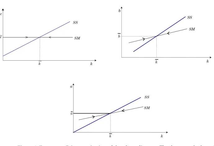
[Insert fig. 1 here]
The geometrical meaning of the former proposition is that the equilibrium points draw a line in a 4-dimensional space. Its local 2-dimensional projections, having k in the abscisses, are all positvely sloped. In particular, it is coincidente with the bisectrix in the (a,k) space. Intuitively, the stock os tastes is positively correlated with the flows of both environmental and non-environmental goods and with financial wealth.
If there is a permanent increase in the relative price of the environmental good, the local projections for c and a will shift up. This means that if there is an increase in π, then there will be some substitution favoring the non-environmental good and the increase in the steady-state expenditure of environmental good should be financed by higher interest income. Alternatively, if there is a permanente increase in labor income then the local projetions for c will remain invariant and the local projection for b will shift down. This means that the increase in labor income will merely substitute interests as a source of financing an invariant level of consumption expendidtures. The symmetry between a and k in the steady-state manifold is not perturbed by any change in the parameters. The slopes of the local projections of the tangent space to the stable manifold are diferent from the local projections of the steady-state manifold.
Proposition 3: (Geometry of the stable manifold)
The local 2-dimensional projections of the stable mainfold are positively sloped in the (a,k) - and (b,k)- spaces and is infinitely sloped in the (c,k) space,
( )
0,1 ) ( ~( ) ~ 1∈ + = ∂ ∂ ρ λ ρ s t k t a (37) 0 ) ( ~( ) ~ = ∂ ∂ t k t c (38)(
)
0 ) ( ~( ) ~ 1 1 > + = ∂ ∂ u s t k t b ρλ λ ρ π (39) Also, while the intercept is invariant for b, it may change for a and c. This is related to the continuity property of the state variables when t tends to zero.To have a complete geometrical analog to the phase diagram, we need to know the relative slopes of the local projections for the stock of financial wealth and the flow-conumption of environmental goods.
Proposition 4: (Realtive slopes of the steady-state and stable manifolds)
The slopes of the local projections of the stable manifold in the (a,k) and (b,k) spaces are flater than the slops of the local projections of the steady-state manifold.
Proof. We get, from equations (21) and (37), 1 0
) ( ~( ) ~ 1 1 − = < + = ∂ ∂ − ∂ ∂ ρ λ ρ λ ρ s s k a t k t a , and from equations (34) and (39), 1
(
(
)
)
0) ( ~( ) ~ 1 1 1 2 1 < + + + = ∂ ∂ − ∂ ∂ cc u aa u cc s u u K u k b t k t b λ δ ρ π λ δ ρ π λ δρ
Obviously the local projections of the steady-sate manifold is steeper than the local projections of the stable maanaifold in (c,k) as the last is horizontal. This means that the consumption of non-environmental goods will display a small degree of inertia, by jumping discontinuously to the new steady-state level after any shock and will be independent from the short-run adjustment of the stock of taste.
The local (a,k) projection of the stable manifold cuts from above the local projection of the steady-state manifold, which is the bisectrix. This means that, near the steady-state, the terminal speed of adjustment for the stock of consumption of environmental goods is larger than that of its flow. The intuition for this is the following. If the flow of consumption of environmental goods changes discontinuously at any moment, then the stock of tastes will also move. If stability prevails, then the stock of taste will (subsequently) continuously vary at a decreasing rate, with the flow of tastes changing at an instantaneously smaller growth rate than the stock. This is a consequence of the assumption of bounded addition: the marginal decrease in the utility flow, more than compensates the inertial effect induced by adjacent complementarity, related to learning-by-consuming, over the stock of tastes.
The intuition on the inconsistency between stock-flow separability and optimality is now straightforward. Consider the opposite: in this case, the dynamics for the consumption of non-environmental goods will be similar to that of the consumption flow of environmental goods. As the model does not have any other dampening effects, then stability would not exist and the objective function could not discriminate between
alternative candidate trajectories for optimality. When there is goods' separability, then the stable trajectory for non-environmental goods is analogous to a model with additive preferences, and it is independent from the short-run dynamics of the environmental good.
5. Applications: Permanent income and relative price
shocks
This section studies the dynamic response of the demand for both environmental and non-environmental goods after a non-anticipated and permanent increases in exogenous income and in the relative price of environmental good.
Proposition 5: (Income shocks)
Let there be a permanent exogenous increase in income. Then:
(1) there will be an initial discontinuously increase in the consumption flow of environmental goods followed by an upward adjustment towards a higher steady-state level. The stock of tastes will change continuously, though at a higher rate of growth. The asymptotic long-run increase in both the consumption flow and the stock of taste will be the same; (2) there will also be an initial increase in non-environmental goods consumption which will remain invariant afterwards; and (3) the stock of non-human wealth will also continuously increase.
Proof. When t = 0 and t = +∞ we get the following expressions for the saddle path
0 ) ( ) 0 ( ~ 1 > + = ∂ ∂ M u K w a π ρ δ cc , ~( ) ( )=− 1( + ) >0 ∂ ∞ ∂ = ∂ ∞ ∂ M u w k w a πρλu ρ δ cc , ~(0) ~( )= 1 1 >0 ∂ ∞ ∂ = ∂ ∂ M u K w c w c λu aa and 0 ) )( ( ) ( ~ 1 2 > + + − = ∂ ∞ ∂ M u w b π ρ δ ρ λs cc , where cc s aa uK u u M 2 2 1 1 1 λπ (ρ δ) λ + + = . The comparative
dynamics expressions for any t are
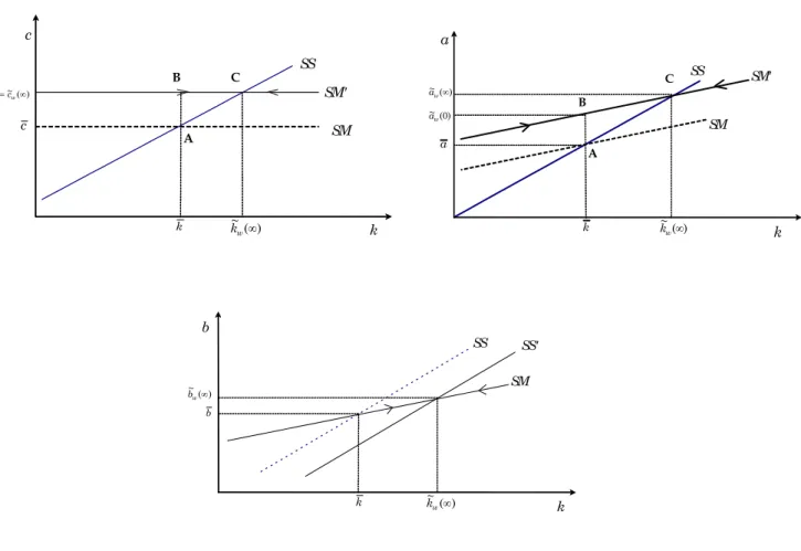
[Insert fig. 2 here]
Figure 2 illustrates the 2-dimensional projections of the perturbed phase diagram. If consumers have a surprise increase in their exogenous income, and if they evaluate it as permanent, then their optimal decisions will be separated as follows. First, they decide on the allocation between steady-state savings and total consumption. Next, they decide how to allocate the total consumption increase between environmental and non-environmental goods. However, as the consumption of non-environmental goods involves a learning-by-consuming process, then consumers have to endure a sluggish increase in the consumption of environmental goods in order to built up their new long-run optimal stock of taste. As far as the non-environmental goods are concerned, they may immediately attain their desired long-run level of consumption.
Proposition 6: (Relative price shocks)
Let there be a permanent exogenous increase in relative price of the environmental goods. Then: (1) there will be an initial discontinuously decrease in the consumption flow of environmental goods followed by a downward adjustment towards a lower steady-state level. The stock of tastes will continuously decay at a higher rate. The asymptotic long-run fall in both the consumption flow and the stock of taste will be the same; (2) if the instantaneously substitution (income) effect dominates then there will be an initial increase (decrease) in non-environmental goods consumption which will
remain invariant afterwards; and (3) the stock of non-human wealth will continuously decrease.
Proof. Now we get ~( ) ( ) =− 1( + )( − ) <0
∂ ∞ ∂ = ∂ ∞ ∂ aa aa b u Mu u p a k a ρλ ρ δ π π π , 0 ) ( ~ ) 0 ( ~ 1 1 < ∂ ∞ ∂ − = ∂ ∂ π ρ λ π k K a u ,
(
)
cc cc u s Mu u a c c 2 2 1 1~( ) ( ) ( ~ ) 0 ( ~ λ λ π ρ δ π π + + − = ∂ ∞ ∂ = ∂ ∂ and(
)
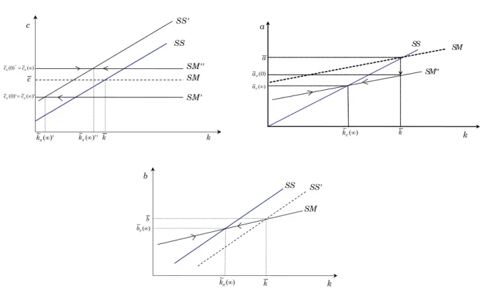
0 ) ( ~ ) ( ~ 1 < ∂ ∞ ∂ + − = ∂ ∞ ∂ π ρ λ ρ λ π π k b u .[Insert fig. 3 here]
A permanent increase in the relative prices of environmental goods will imply a long-run reduction in real income. Therefore, in their two-stage decision process, the representative consumer will both reduce its long-run consumption and savings. However, the consumption reallocation between environmental/non-environmental goods will involve both substitution and income effects. While income effect reduces both consumption's, the substitution effect shifts demand from environmental to non-environmental goods. Then, non-non-environmental goods consumption will increase or decrease depending upon which effect (income or substitution) dominates: if income effect dominates then there will be a decrease in the consumption of non-environmental goods, but if the substitution effect dominates then there could be an increase in non-environmental goods consumption.
Additionally, environmental goods consumption will unambiguously fall because of both income and substitution effects. However, we may infer from figure 3 that if income effect dominates we would expect a much larger reduction in the steady-state consumption of environmental goods. The short-run dynamics will be symmetric as regards an increase in exogenous income.
6. Conclusions
In this paper we offer a thorough examination of the canonical model of environmental economics. Two main contributions should be stressed. First, we prove that the learning-by-consuming process will only be consistent with a preference structure involving environmental/non-environmental intratemporal separability, for an optimal solution to exist. Second, under the assumptions of bounded adjacent complementarity, we explicitly derived the geometrical characteristics of the steady-state, stable manifolds and their deformations for permanent and non-anticipated changes in both income and relative price of environmental goods.
The following main conclusions should be emphasized. First, there is instantaneous complementarity between the stock of tastes and financial wealth. Second, an increase in real income will lead to an increase in the stock of taste and, therefore, to an increase in the flow-demand for environmental goods. Third, the demand for environmental goods will be reduced through both income and substitution effects, if the relative price increases.
References
Becker, G. S. and Murphy, K. M. (1988); A Theory of Rational Addition, Journal of Political Economy, 96, 675-700.
Braden, J. B. and Kolstad, C. D, Ed. (1991); Measuring the demand for environmental quality, North-Holland.
Brito, P. (1997); Local dynamics for planar optimal control problems: a complete characterization, Working paper 7/97, Department of Economics, ISEG, Technical University of Lisbon.
Kamien, M and Schwartz, N (1991); Dynamic Optimization, 2nd ed., North-Holland.
Krisntöm B. and Riera, P (1996); Is the income elasticity of environmental improvements less
than one?, Environmental & Resources Economics, 7(1), 45-55.
Lucas, R. (1988); On the Mechanics of Economic Development, Journal of Monetary Economics, 22(1), 3-42.
Mccain, R. (1995); Cultivation of taste and bounded rationality: some computer simulations, Journal of Cultural Economics, 19(1), 1-15.
Mansoorian, (1993); Habit Persistence and the Hargerber-Laursen-Metzler Effect in an Infinite
Horizon Model, Journal of International Economics, 34, pp. 153-166
Mansoorian, (1998); Habits and Durability in Consumption, and Dynamics of the Current
Account, Journal of International Economics, 44, pp 69-82.
Ryder, H. E. and Heal, G. M. (1973); Optimum growth with intertemporally dependent
preferences, Review of Economics Studies, 40, 1-33.
Stigler, G. and Becker, G. (1977); De gustibus non est disputandum, American Economics Review, 67(1), 76-90.
Figure 1: Exogenous Prices: projection of the phase diagram. The three panels show the two-dimensional projections of the Steady-State Manifold (SS) and of the Stable Manifold (SM),in the neighborhood of an equilibrium point (c ,b ,k , a). It does not contain the representations of the projections of all the nullclines. As the dynamics in the neighborhood of the steady state is equivalent to that of a linear model, the figure only represent the linear approximations.
k a SS SM k a k c c SS SM k k b SS SM k b
Figure 2: Exogenous prices: effects of a permanent shock in income, w. A non-anticipated permanent increase in exogenous income, will cause an immediate rightward shift in local two-dimensional projection of the steady-state manifold in the (a,k)-axis, leaving the other two unchanged. However, the local projections of the stable manifold will shift upwards in (c,k) and the (b,k)-axis.
k c SS SM SM' c k k~ ∞w( ) ) ( ~ ) 0 ( ~ = ∞ w w c c A B C k a SS SM SM' ) ( ~ ∞w a ) 0 ( ~ w a a k k~ ∞w( ) A B C k b SS SM ) ( ~ ∞w b b k k~ ∞w( ) SS'
Figure 3: Permanent shock in the relative price k c SS SM' SM c k SS' SM'' '' '' ~( ) ) 0 ( ~π =cπ∞ c )' ( ~ )' 0 ( ~π =cπ∞ c )' ( ~ ∞π k k~ ∞π( )'' k a SS SM SM'' a k ) 0 ( ~ π a ) ( ~ ∞π a ) ( ~ ∞π k k b SS SM b k SS' ) ( ~ ∞π b ) ( ~ ∞π k