Parallel local search for the Costas Array Problem
Daniel Diaz∗, Florian Richoux†, Yves Caniou‡, Philippe Codognet†, Salvador Abreu§
∗ Universit´e de Paris 1-Sorbonne, France
Daniel.Diaz@univ-paris1.fr
† JFLI, CNRS / UPMC / University of Tokyo, Japan
{richoux, codognet}@is.s.u-tokyo.ac.jp
‡ JFLI, CNRS / NII, Japan
Yves.Caniou@ens-lyon.fr
§ Universidade de ´Evora and CENTRIA FCT/UNL, Portugal
spa@di.uevora.pt
Abstract—The Costas Array Problem is a highly combina-torial problem linked to radar applications. We present in this paper its detailed modeling and solving by Adaptive Search, a constraint-based local search method. Experiments have been done on both sequential and parallel hardware up to several hundreds of cores. Performance evaluation of the sequential version shows results outperforming previous implementations, while the parallel version shows nearly linear speedups up to 8,192 cores.
I. INTRODUCTION
During the last decade, the family of Local Search meth-ods and Metaheuristics has been quite successful in solving large real-life problems [22], [23], [24]. Applying Local Search to Constraint Satisfaction Problems (CSP) has also been attracting some interest [9], [18], [23], [25] as it can tackle CSPs instances far beyond the reach of classical propagation-based solvers.
A generic domain-independent Local Search method named Adaptive Search was proposed in [9], [10]. It is a metaheuristic that takes advantage of the structure of the problem to guide the search and that can be applied to a large class of constraints (e.g., linear and non-linear arithmetic constraints and symbolic constraints). Moreover, it intrinsically copes with over-constrained problems.
We will describe in this paper how the Costas Array Prob-lem can be modeled easily in the Adaptive Search framework and how this model can be refined progressively in order to achieve very good performances on sequential machines. The Costas Arrays Problem (CAP) has been introduced to the constraint programming community in [25]. It is an abstract problem that was motivated by a sonar application in the 1960’s but still has practical interest in radar and software-defined radio applications [3]. A whole community is active around the CAP (http://www.costasarrays.org) as several problems are not yet solved, e.g., no constructive algorithm exists for larger values of n and the question of the existence of a Costas array of size n for n = 32 is still open. From a constraint programming point of view, it is an interesting problem because CAP is conceptually related
to three well-known CSPs: the perennial N queens problem, the All-Interval Series problem (prob007 of CSPLib [19]), and the Golomb rulers problem (prob006 of CSPLib), but it is much more difficult to solve, mainly because of a tricky, bi-dimensional alldifferent constraint.
When attacking a highly combinatorial problem, an inter-esting approach is also to consider parallel implementations in order to boost performance. In the last decade, with desktop computers turning into parallel machines with 2, 4 or even 8 core CPUs, designing and implementing efficient parallel constraint solvers has become an increasingly devel-oping research field. However, only a few efficient parallel implementations of constraint solvers have been reported, e.g.,the seminal work of [34], [35] on quad-core machine and the Comet system [23] which has been parallelized for small clusters of PCs, both for its local search solver [28] and its propagation-based constraint solver [29]. Recent experiments have been done up to 12 processors [30], and speedups tend to level off after 10 processors. It has to be noted that it is not obvious how to scale such implemen-tations up to a few hundreds of processors, either because of the shared-memory nature of the solver or because of the intrinsic sequentiality of the solving method or of the problem itself.
In [13], [7], [6], a parallel version of a constraint solver based on local search is defined with a multi-start approach requiring no communication between processes (also known as Pleasantly Parallel). On classical CSP benchmarks from CSPLib, this simple parallelization scheme gives good re-sults, with a factor 50-70 speedup for 256 cores, but this is far from ideal speedup (e.g., factor 256 speedup for 256 processors), even for large problem instances. It is thus an open question to know whether this is due to the classical (structured) CSP benchmarks used or if this is a limitation of the method. In this paper we address the problem of modeling a very combinatorial problem, with a low density of solutions (the CAP) in the sequential version and we further investigate if it scales up to a large number of processors and exhibits better speedups. For this we
used three platforms: (1) the HA8000 machine, an Hitachi supercomputer with 15,232 cores installed at University of Tokyo, (2) the GRID’5000 infrastructure, the French national Grid for the research, which contains a total of 8,596 cores deployed on 9 sites distributed in France and (3) the IBM Blue Gene/P machine JUGENE with 294,912 cores at the J¨ulich Supercomputing Center in Germany. Experiments on both HA8000 and GRID’5000 show nearly linear speedups w.r.t. the sequential version, for instance 120 for 128 cores and 230 for 256 cores. On the Blue Gene/P, we obtained linear speed-ups up to 8,192 cores.
The rest of this paper is organized as follows. Section II presents the Costas Array Problem and Section III the Adaptive Search method. Section IV presents the mod-eling of the Costas Array Problem within the Adaptive Search formalism, and the performance of the sequential implementation. Section V details the experiments on three different parallel hardware: the HA8000 supercomputer, the GRID’5000 platform and the Blue Gene/P supercomputer. Section VI concludes the paper and briefly discusses about future work.
II. THECOSTASARRAYPROBLEM
A Costas array is an n × n grid containing n marks such that there is exactly one mark per row and per column and the n(n − 1)/2 vectors joining the marks are all different. We give here an example of Costas array of size 5. It is convenient to see the Costas Array Problem (CAP) as a permutation problem by considering an array of n variables (V1, . . . , Vn) which forms a permutation of
{1, 2, . . . , n}. The Costas array above can thus be repre-sented by the array [3, 4, 2, 1, 5].
Historically, these arrays have been developed in the 1960’s to compute a set of sonar and radar frequencies avoiding noise [11]. A very complete survey on Costas arrays can be found in [14]. The problem to find a Costas array of size n is very complex since the required time grows exponentially with n. In the 1980’s, several algorithms have been proposed to build a Costas array given n, such as the Welch construction [20] and the Golomb construction [21], but these methods cannot built Costas arrays of size 32 and some higher non-prime sizes. Nowadays, after many decades of research, it remains unknown if there exist any Costas arrays of size 32 or 33. Another difficult problem is to enumerate all Costas arrays for a given size. Using the Golomb and Welch constructions, Drakakis et. al present in [16] all Costas arrays for n = 29. They show that among the 29! permutations, there are only 164 Costas arrays, and 23 unique Costas arrays up to rotation and reflection. There are constructive methods known to produce Costas arrays of order 24 to 29 [4], [38], [15], [16].
The Costas Array Problem has been proposed as a chal-lenging combinatorial problem by Kadioglu and Sellmann in
[25]. They propose a local search metaheuristic, Dialectic Search, for constraint satisfaction and optimization, and show its performance for several problems. Clearly this problem is too difficult for propagation-based solvers, even for medium size instances (i.e., with n around 18 − 20). Let us finally note that we do not pretend that using local search is better than constructive methods in order to solve the CAP. We rather consider the CAP as a very good benchmark for testing local search and constraint-based systems and to investigate how they scale up for large instances and parallel execution.
In [37], Rickard and Healy studied a stochastic search method for CAP and concluded that such methods are unlikely to succeed for n > 26. Although their conclusion is true for their stochastic method, it cannot be extended to all stochastic searches: their method uses a restart policy which is too simple and they also used an approximation of the Hamming distance between configurations in order to guide the search which they recognized themselves not be be a very good indicator. However, they studied in this paper the distribution of solutions in the search space and have shown that clusters of solutions tend to spread out from n > 17, which justify our multi-walk approach presented in Section V to reach linear speedup for high values of n.
III. THEADAPTIVESEARCHMETHOD
Adaptive Search (AS) was proposed in [9], [10] as a generic, domain-independent constraint-based local search method. This metaheuristic takes advantage of the structure of the problem in terms of constraints and variables and can guide the search more precisely than a single global cost function to optimize, such as for instance the number of violated constraints. The algorithm also uses a short-term adaptive memory in the spirit of Tabu Search in order to prevent stagnation in local minima and loops.
A. Algorithm
The input of the method is a problem in CSP format: a set of variables with their (finite) domains of possible values and a set of constraints over these variables. For each constraint, an error function needs to be defined: it gives, for each tuple of variable values, an indication of how much the constraint is violated. Consider an n-ary constraint c(X1, · · · Xn) and
associated domains D1, · · · , Dn for each variable. An error
function fc associated to the constraint c is a real-valued
function from D1× · · · × Dn such that fc(X1, · · · Xn) has
value zero iff c(X1, · · · Xn) is satisfied. The error function
will in fact be used as a heuristic to represent the degree of satisfaction of a constraint and will thus give an indication on how much the constraint is violated. This idea has also been proposed independently by [18], where it is called ”penalty functions”, and then reused in the Comet system [23], where it is called ”violations”. For example, the error function associated with an arithmetic constraint |X − Y | < c, for
a given constant c ≥ 0, can be max(0, |X − Y | − c). AS relies on iterative repair, based on variable and constraint error information, seeking to reduce the error on the worst variable so far. The basic idea is to compute the error function for each constraint, then combine for each variable the errors of all constraints in which it appears, thereby projecting constraint errors onto the relevant variables. This combination of errors is problem-dependent, see [9] for details and examples, and represents the heuristic distance to a solution. It is usually a simple sum of absolute values, i.e.,Manhattan distance, although it might also be any other distance or maybe a weighted sum if constraints are given different priorities. Finally, the variable with the highest error is designated as the “culprit” and its value is modified. In this second step, the well known min-conflict heuristic [31] is used to select the value in the variable domain which is the most promising, that is, the value for which the total error in the next configuration is minimal. In order to prevent being trapped in local minima, the AS method also includes a short-term memory mechanism to store configurations to avoid. More precisely, variables can be marked Tabu and “frozen” for a given number of iterations. It also integrates reset transitions to escape stagnation around local minima, see Section III-B. As in every local search method, it is also possible to restart from scratch when the number of iterations becomes too large. The AS base algorithm is described in Figure 1.
Adaptive Search is a simple algorithm but it turns out to be quite efficient in practice. As a simple comparison, [6] provides timings between AS and the Comet 2.1.1 system on a few classical benchmarks. AS is about 40 times faster than Comet on the N-queen problem (for N =10000 to 50000) and 100 to 500 times faster than Comet for the Magic Square problem (prob019 in CSPLib), for N =30 to 50. Of course, it should be noted that Comet is a complete and very versatile system while AS is just a C-based library. In [25] a new metaheuristics named Dialectic Search is compared with the 2001 version of AS [9], showing that both methods have similar results for the Magic Square problem (instances from N =20 to 50). However when compared with the 2003 version of AS [10], AS is about 15 to 40 times faster than Dialectic Search (depending on the instances), on the same reference machine. Obviously, performance comparisons are always tricky, but one or two orders of magnitude can be considered as significant, especially as speedups increase with problem size. The basic code for permutation problems and examples are available as free software at the URL: http://cri-dist.univ-paris1.fr/diaz/adaptive/
B. Tuning Adaptive Search
1) Plateaux: In [10], a simple but very effective improve-ment of the original algorithm was proposed. In AS, when a variable is selected and all alternative values for this variable give a global cost worse than the current one, this variable is
tagged as ”Tabu” for a given number of iterations. However, what should be done when there is no improvement, but only equal-valued moves? In that case, a ”plateau” is found in the global cost function landscape, and the question is to either follow this plateau or not. A simple idea is to introduce a probability p for this. With a good tuning (e.g., probability of 90% to 95% of following a plateau) this boosts the performance of the algorithm by an order of magnitude on some problems such as Magic Square. Indeed the current sequential AS version of Magic Square problem can solve instances as big as 400x400 (i.e., 160,000 variables with domains of size 160,000) in about one hour on average.
2) Reset: When too many variables become Tabu, there is a risk of ”freezing” the configuration and of getting trapped around a local minimum. The AS method thus needs a diversification operator to avoid such cases. This is done by performing a (partial) reset, i.e., by assigning fresh values to a given percentage of the problem variables (parameter RP of the algorithm). A reset is triggered by the total number of variables being marked Tabu at a given iteration (parameter RL of the algorithm). This is the generic default reset mechanism of AS, but the reset procedure can also be customized if needed to become dedicated to a given problem. We use this ability for solving efficiently the CAP. 3) Random: Using a reliable pseudo-random number generator is essential for local search algorithms. For se-quential methods, using generic random functions provided by standard libraries is often good enough. However, the need for better random functions (i.e., more uniform) already appeared in stochastic optimization methods such as Particle Swarm Optimization (PSO) [40]. Therefore, when designing a massively parallel method with several hundreds or thou-sands of stochastic processes running at the same time, one has to choose carefully their random seed and to be assured of the correctness of the distribution. At this point, using a generic random function can turn out to be insufficient.
To ensure equity, we choose to generate the seed used by each process via a pseudo-random number generator based on a linear chaotic map. This method shows robust properties of distribution and has been implemented for cryptographic systems, like Trident [32].
IV. SOLVING THECAPWITHADAPTIVESEARCH
A. Basic Model
The CAP can be modeled as a permutation prob-lem by considering an array of n variables (V1, . . . , Vn)
which forms a permutation of {1, 2, . . . , n} (i.e., implicit alldifferent constraint on variables Vi). Vi = j iff
there is a mark at column i and row j. To take into account constraints on vectors between marks (which must be different) it is convenient to use the so-called difference triangle.
This triangle contains n−1 rows, each row corresponding to a distance d. The dth row of the triangle contains the
Figure 1. Adaptive Search Base Algorithm
differences Vi+d− Vi for all i = 1, . . . , n − d (i.e., the
difference of values at a distance d). Ensuring all vectors are different comes down to ensure the triangle contains no repeated values on any given row (i.e., alldifferent constraint on each row). Here is the difference triangle for the Costas array given as example in Section II.
3 4 2 1 5
d = 1 1 -2 -1 4
d = 2 -1 -3 3
d = 3 -2 1
d = 4 2
In AS, the way to define a constraint is done via error
functions. At each new configuration, the difference triangle is checked to compute the global cost and the cost of each variable Vi. Each row d of the triangle is checked one by
one. Inside a row d, if a pair (Vi, Vi+d) presents a difference
which has been already encountered in the row, the error is reported as follows: increment the global cost and the cost of both variables Viand Vi+dby ERR(d) (a strictly positive
function). For a basic model we can use ERR(d) = 1 (to simply count the number of errors). Obviously a solution is found when the global cost equals 0. Otherwise AS selects the most erroneous1 variable and will try to improve it.
B. Optimization
In the basic model, the function ERR(d) can be a constant (e.g., ERR(d) = 1) but a better function is ERR(d) = n2−d2which “penalizes” more errors occurring
in the first rows (those containing more differences). The use of this function instead of ERR(d) = 1 improves the computation time (around 17 %).
Moreover, a remark from Chang [8] makes it possible to focus only on distances d ≤ b(n − 1)/2c. In our example, it is only necessary to check the 2 first rows of the triangle (i.e., d = 1 and d = 2). This represents a further gain in computation time (around 30 %).
Another source of optimization concerns the reset phase. Recall that AS maintains a Tabu list to avoid to be trapped in local minima and, when too many variables become Tabu, the current configuration is perturbed to escape the current local minimum. By default AS resets a certain percentage of variables (see parameters RL and RP in the previous algorithm). We found good results with RL = 1 and RP = 5% (as soon as 1 variable is marked Tabu, reset 5% of the variables). Whereas this default behavior of AS is general enough to escape any local minimum, it sometimes “breaks” some important parts of the current configuration (but conversely, if we want to preserve too many variables, we can be trapped in the local minimum). AS allows the user to define his own reset procedure: when a reset is needed this procedure is called to propose a pertinent alternative configuration. Our customized reset procedure tries 3 different perturbations from the current configuration: 1) Select the most erroneous variable Vm. Consider each
sub-array starting or ending by Vmand shift it
(circu-larly) from 1 cell to the left and to the right.
2) Add a constant “circularly” (i.e., modulo n to maintain the permutation) to each variable. The current imple-mentation tries the following 4 constants: 1, 2, n − 2, n − 3 (but middle values n/2, n/2 − 1, n/2 + 1 are also pertinent).
3) Left-shift from 1 cell the sub-array from the beginning to a (randomly chosen) erroneous variable different from Vm. In the current implementation we test at
most 3 erroneous variables.
As soon as the global cost of a perturbation is strictly inferior to the entry global cost the local minimum is considered as escaped and AS continues with this (perturbed) con-figuration. This works, on average, in 32% of the cases (independently from n). Otherwise, all perturbations are tested exhaustively and the best (i.e., whose global cost is minimal) is selected. This dedicated reset procedure provides a speedup factor of about 3.7 and is thus very effective. C. Evaluation of the sequential implementation
In this section we study the performances of the sequential AS implementation. Since AS is a stochastic method and
uses randomness for initial configurations and during its execution, each benchmark has been executed 100 times. Classically, there are three interesting ways for aggregating those results: considering the best case, the worst case and the average case (i.e., minimum, maximum and average of 100 execution times). The experiments were run on a Dell Precision T7500 (Intel Xeon W5580, 3.20 GHz and 24 GB of 1333MHz SDRAM) running Linux (the AS code is compiled using GCC 4.4.5, with the -O3 flag).
Size Time Iterations Local min ratio 16 avg 0.08 12665 6853 min 0.00 212 117 60 max 0.45 69894 37904 17 avg 0.59 73430 38982 min 0.02 2591 1361 30 max 2.39 294580 156154 18 avg 3.49 395838 207067 min 0.03 2789 1538 116 max 19.81 2254001 1178875 19 avg 29.46 2694319 1372671 min 0.31 28911 14798 95 max 127.78 11619940 5922204 20 avg 250.68 20536809 10278723 min 3.89 319368 159127 66 max 1097.06 89791761 44945485 Table I
EVALUATION OF THE SEQUENTIAL IMPLEMENTATION(TIMES IN SEC.)
Table I presents the results of the evaluation. For each in-stance it details the execution time (in seconds), the number of iterations, the number of local minima encountered and the ratio between the average time and the minimum time (when the minimum time is zero we used the numbers of iterations). For n = 18 and above, an exponential behavior seems to appear: the computation time for solving instance n is an order of magnitude greater than n − 1. More interestingly, for all instances, the best case is much faster than the average case (see last column of Table I). This important property convinced us to experiment on parallel machines as we will see later.
In [25], Kadioglu and Sellmann propose a novel and in-teresting local search meta-heuristic called Dialectic Search (DS). The authors show how DS performs well on the CAP and compare DS with a tabu search algorithm using the quadratic neighborhood implemented in Comet. The comparison was done for instances 13 to 18 and revealed that DS is between 2 and 3 times faster than Comet on CAP. It is thus very interesting to compare our AS implementation with DS. The comparison was however difficult because Kadioglu and Sellmann used an outdated machine and no rigorous scaling information is available to compare their Pentium-III 733 MHz with modern processors. Fortunately we managed to find an exactly identical machine. The following table presents the comparison with DS considering for both systems the average of 100 executions. Times are given in seconds measured on a Pentium-III 733 MHz for AS and taken from [25] for DS.
Size DS AS DS / AS 13 0.05 0.01 5.00 14 0.26 0.05 5.20 15 1.31 0.24 5.46 16 7.74 0.97 7.98 17 53.40 7.58 7.04 18 370.00 44.49 8.32 Table II ASSPEED-UPS W.R.TDS
Unfortunately, the paper about DS does not give other data than time executions, therefore we are not in measure to compare the number of iterations, local minima, etc. This table clearly shows that AS outperforms DS on the CAP: for small instances AS is five times faster but the speedup seems to grow with the size of the problem, reaching a factor 8.3 for n = 18.
CAP has also been used as a benchmark in the Constraint Programming community and we can compare with a CP Comet program made by Laurent Michel and based on the modeling in MiniZinc by Barry O’Sullivan2. As could be expected, CP is much less efficient than local search, and this Comet program is about 400 times slower than Adaptive Search for CAP19.
V. PARALLELIMPLEMENTATION ANDPERFORMANCE
ANALYSIS
Parallel implementation of local search metaheuristics have been studied since the early 90’s, when multiprocessor machines started to become widely available, see [39] for a general survey and concepts, or [33] for basic parallel versions of Tabu search, simulated annealing, GRASP and genetic algorithms. With the availability of clusters in the early 2000’s, this domain became active again [12], [2]. Apart from domain-decomposition methods and population-based method (such as genetic algorithms), one usually distinguishes between single-walk and multiple-walk meth-ods for Local Search. Single-walk methmeth-ods consist in us-ing parallelism inside a sus-ingle search process, e.g., for parallelizing the exploration of the neighborhood, see for instance [26] for such a method making use of GPUs for the parallel phase. Multiple-walk methods (also called multi-start methods) consist in developing concurrent explorations of the search space, either independently or cooperatively with some communication between concurrent processes. A key point is that independent multiple-walk methods are the easiest to implement on parallel computers and can lead to linear speed-up if solutions are uniformly distributed in the search space and if the method is able to diversify correctly [39]. However, previous experiments [6] showed that on structured problems such as (non-random) CSPs, independent multiple-walk parallelization does not achieve
2http://www.g12.cs.mu.oz.au/mzn/costas array/CostasArray.mzn
ideal speedups, reaching only a factor 50-70 speedup for 256 cores. It might be because solutions are not uniformly dis-tributed in the search space, and are for instance regrouped in ”clusters”, as was shown for solutions of SAT problems near the phase transition in [27]. Therefore some sequential computation is needed to get to the vicinity of such clusters. A. Motivation and Implementation
As remarked in Section IV-C, it can be seen than in 100 sequential runs of the algorithm starting from different (random) initial configurations, the minimal one is much faster than the average (sometimes more than 100 times). Then if we can run in parallel many AS engines we can hope for a global execution time equal to the minimal one, and therefore a good speedup.
We implemented a parallel version of AS using Open-MPI, an implementation of the MPI standard [17]. Pre-liminary experiments and performance results on classical CSP benchmarks are described in [6]. The parallelization is straightforward and based on the idea of multi-start and independent multiple-walk: fork a sequential AS method on every available cores. But on the opposite of the classical fork-join paradigm, parallel AS shall terminate as soon as a solution is found, not wait until all the processes have finished (since some searches initialized with ”bad” initial configurations can take some time). Thus, some non-blocking tests are involved every c iterations to check if there is a message indicating that some other process has found a solution; in which case it terminates the execution properly. This results in a high number of independent work units, a high CPU to I/O ratio, and no inter-process communication for computation.
Four different testbeds were used on three platforms:
• HA8000, the Hitachi HA8000 supercomputer of the
University of Tokyo with a total number of 15,232 cores. This machine is composed of 952 nodes, each of which is composed of 4 AMD Opteron 8356 (Quad core, 2.3 GHz) with 32 GB of memory. Nodes are interconnected with a Myrinet-10G network attaining 5 GB/s in both directions. HA8000 can theoretically achieve a performance of 147 Tflops, but we only accessed to a subset of its nodes as users can only have a maximum of 64 nodes (1,024 cores) in normal service.
• GRID’5000 [5], the French national Grid for research, which consists of 8,596 cores deployed on 9 sites in France. We used two subsets of the computing re-sources of the Sophia-Antipolis node: Suno, composed of 45 Dell PowerEdge R410 with 8 cores each, thus a total of 360 cores, and Helios, composed of 56 Sun Fire X4100 with 4 cores each, thus a total of 224 cores.
• JUGENE, the IBM Blue Gene/P supercomputer at
the J¨ulich Supercomputing Center containing 294,912 cores. This machine is composed of 73,728 nodes, each
of which is composed of 4 Power PC 450 32-bits at 850Mhz with 2 GB of memory. The network is a 3-dimensional torus reaching a bandwidth of 5.1GB/s. The overall peak performance is 1 Pflops.
B. Experiments on parallel machines
Let us now present the result of the parallel experiments. The following tables show the execution times on HA8000 (Table III), JUGENE (Table IV) and GRID’5000 (Table V). Execution times do not include the deployment time, negli-gible on big benchmarks. Behaviors on both platforms are similar and exhibit good speedups. We give the timings in seconds for 50 executions of each benchmark with the average time, median time, minimal time and maximal time. We can see that with more cores, the maximal time decreases a lot and thus the difference between minimal and maximal times decreases. Moreover, in our case the median time is always below the average time, meaning we have more fast runs rather than slow ones. The median time presents here a speedup at least as good as the average time. For instance, for n = 20 and using 256 cores on HA8000, speedup obtained w.r.t sequential runs is a factor 170 concerning the average time and a factor 210 for the median time.
Size 1 core 32 cores 64 cores 128 cores 256 cores
18 avg 6.76 0.25 0.23 0.24 0.26 med 4.25 0.18 0.18 0.20 0.23 min 0.23 0.00 0.00 0.00 0.00 max 22.81 1.07 0.90 0.94 0.78 19 avg 54.54 1.84 1.00 0.72 0.55 med 43.74 1.45 0.76 0.57 0.44 min 0.51 0.0 0.03 0.02 0.01 max 212.96 6.62 5.24 3.48 2.22 20 avg 367.24 13.82 8.66 3.74 2.18 med 305.79 11.53 5.06 2.36 1.44 min 9.51 0.05 0.03 0.03 0.06 max 1807.78 54.26 36.98 23.87 9.21 21 avg - 160.42 81.72 38.56 16.01 med - 114.06 53.04 30.68 10.12 min - 1.63 2.13 1.49 0.73 max - 654.79 335.66 145.59 93.13 22 avg - 501.23 249.73 128.47 60.80 med - 450.45 178.85 99.62 55.90 min - 0.23 0.35 0.26 1.58 max - 1550.25 935.51 406.15 196.26 Table III
EXECUTION TIMES(IN SEC.)ONHA8000
For small instances (n = 18), since computation times of parallel executions on many cores are below 0.5 second, they are maybe not significant because of interactions with operating system operations.
For medium instances, we have for example a 226 times speedup w.r.t. sequential execution on Suno for n = 19 on 256 cores. Indeed, for different CAP instances, speedups w.r.t. sequential version are between 75 and 120 on 128 cores on HA8000, and between 100 and 170 on 256 cores on HA8000, between 120 and 137 on 128 cores on Suno, between 204 and 226 on 256 cores on Suno and between 120 and 130 on 128 cores on Helios.
Size 512 cores 1,024 cores 2,048 cores 4,096 cores 8,192 cores
21 avg 43.66 27.86 10.21 5.97 2.84 med 30.31 23.67 5.56 4.47 2.07 min 0.85 1.46 0.27 0.13 0.19 max 274.69 108.14 93.89 21.98 12.92 22 avg 265.12 148.80 76.24 36.12 20.00 med 166.47 79.63 63.24 28.00 13.41 min 1.34 1.95 0.81 0.60 0.30 max 1831.96 638.34 277.96 154.89 84.66 23 avg - - 633.09 354.69 170.38 med - - 522.68 213.22 124.67 min - - 2.41 9.32 4.94 max - - 3527.80 1873.07 748.29 Table IV
EXECUTION TIMES(IN SEC.)ONJUGENE
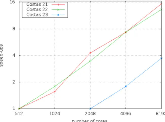
For bigger instances, such as n = 21 and 22, we do not have timings on HA8000 for the sequential version because a sequential problem resolution takes on average more than one hour, and the maximum resource utilization is currently limited to one hour because of power savings. For n = 21 on Suno we have a 218 times speedup on 256 cores w.r.t. sequential execution. Concerning n = 22, as sequential computation takes many hours, we limit our experiments on all machines to executions on 32 cores and above. Therefore in Figure 2, we will only give timings from 32 to 256 cores. On JUGENE, we ran our experiments starting from 512 cores. Indeed, despite HA8000 processors or Grid’5000 processors at 2.4Ghz, Blue Gene/P processors have a low frequency (850 Mhz), and are then significantly slower to solve a given problem. Moreover, JUGENE’s job scheduler forces a time-out of 30 minutes for any job using less than 1025 cores, which made difficult on few cores our experiments which require 50 runs each. This is why we started experiments on JUGENE from 512 cores for n = 21 and n = 22 and from 2,048 cores for n = 23. For these two instances, one can see we reach nearly linear speed-ups up to 8,192 cores : We have a speed-up of 15.33 for n=21 w.r.t executions over 512 cores (perfectly linear speed-up would be 16), and of 13.25 for n=22 w.r.t executions over 512 cores. Finally, we obtain a speed-up of 3.71 for n=23 w.r.t executions over 2,048 cores, very near to a perfect linear speed-up of 4. Details about speed-ups on the JUGENE machine are represented by Figure 3. We can see that on all platforms, execution times are halved when the number of cores is doubled, thus achieving ideal speed-up.
This is graphically depicted in the next figure on a log-log scale. As a final result, we note that we can now solve n = 22 in about one minute on average with 256 cores on HA8000. We can explain these linear speed-ups due to the good distribution of solution clusters over the search space for n > 17 as shown in [37]. Thus, parallel searches using a multi-start approach greatly increase its chance to start near from a solution.
Up to now, we focused on the average execution time in order to measure the performance of the method, but a
Suno Helios
Size 1 core 32 cores 64 cores 128 cores 256 cores 1 core 32 cores 64 cores 128 cores
18 avg 5.28 0.16 0.083 0.056 0.038 8.16 0.24 0.11 0.06 med 0.11 0.065 0.04 0.03 0.19 0.06 0.04 min 0.01 0.00 0.00 0.00 0.0 0.13 0.00 0.00 0.00 max 20.73 0.64 0.34 0.19 0.13 37.5 1.08 0.46 0.26 19 avg 49.5 1.37 0.59 0.41 0.219 52 2.3 0.87 0.40 med 1.09 0.38 0.33 0.155 1.27 0.60 0.25 min 0.67 0.02 0.01 0.00 0.02 0.72 0.05 0.0 0.01 max 279 9.41 2.74 1.82 1.12 234.45 10 4.14 2.11 20 avg 372 12.2 5.86 2.67 1.79 444 14.3 7.63 4.52 med 10.6 4.63 2.01 1.16 8.28 5.16 2.76 min 4.45 0.14 0.07 0.0 0.01 5.71 0.21 0.01 0.01 max 1456 50.6 26 19.2 8.5 2540 139 41.7 18.7 21 avg 3743 171 51.4 34.9 17.2 5391 153 101 36.7 med 108 38.5 21.8 10.8 111 68.6 24.1 min 265 5.56 0.24 0.27 1.05 96.6 2.18 0.45 0.29 max 10955 893 235 173 63.3 18863 657 560 161 22 avg - 731 381 200 103 - 1218 520 220 med - 428 286 135 69.5 - 819 276 133 min - 24.7 13.1 5.23 2.17 - 78.9 4.12 3.01 max - 6357 1482 656 451 - 4635 3184 1670 Table V
EXECUTION TIMES(IN SEC.)ONGRID’5000 (SUNO ANDHELIOS)
Figure 2. Speed-ups (HA8000 - Grid’5000) for CAP 22 w.r.t. 32 cores
more detailed analysis could be done. In [1], [36], a method is introduced to represent and compare execution times of stochastic optimization methods by using so-called time-to-target plots. Observe that, for the CAP, the time-to-target value to achieve is obviously zero, meaning that a solution is found. It is then easy to check if runtime distributions could be approximated by a (shifted) exponential distribution of the form: 1 − e−(x−µ)/λ. Then, according to [39], it is possible to achieve linear speed-ups by multiple independent walks if we have an exponential runtime distribution.
Figure 4 presents time-to-target plots for CAP 21 in order to compare runtime distributions over 32, 64, 128 and 256 cores.
Points represent execution times obtained over 200 runs and lines correspond to the best approximation by an expo-nential distribution. It can be seen that the actual runtime
Figure 3. Speed-ups on the JUGENE for CAP 21, 22 and 23
distributions are very close to exponential distributions. Time-to-target plots also give a clear visual comparison between instances of the same method running on a different number of cores. For instance it can be seen that we have around 50% chance to find a solution within 100 seconds using 32 cores, and around 75%, 95% and 100% chance respectively with 64, 128 and 256 cores.
VI. CONCLUSION AND FUTURE WORK
We detailed the modeling and solving of the CAP with the Adaptive Search method. The CAP is a hard combinatorial problem for medium and large instances, too difficult to solve with classical propagation-based solver and we thus used a constraint-based local search solver. We presented a simple modeling and have shown how to further tune the resolution within the Adaptive Search framework. Careful
Figure 4. Time-to-Target plots for CAP 21 over 32, 64, 128 and 256 cores
modeling and tuning, together with an efficient paralleliza-tion, achieved very good performance. We proposed a paral-lel version based on the idea of multi-start and independent multiple-walk which naturally provides Pleasantly Parallel computations and appears viable as it exhibits a nearly linear speed-up behavior. Indeed, we obtained speed-ups w.r.t. sequential implementation of 120 for 128 cores and 226 for 256 cores for medium instances, i.e., nearly linear. For the largest instances studied in this paper (CAP 22 and 23), execution times are halved when the number of cores is doubled from 32 cores onward for CAP 22 (from 512 cores on the Blue Gene/P), and linear speed-ups can be observed up to 8,192 cores. Experiments for CAP 23 was only possible on the Blue Gene/P starting from 2,048 cores, and scales also up to 8,192 cores. We are currently continuing our experiments by tackling larger instances and using more cores.
Future work will focus on more complex parallel ex-ecution methods with inter-processes communication, i.e., in the dependent multiple-walk scheme, in order to further improve performance. The communication mechanism will be designed with the goals of (1) minimizing data transfers as much as possible, as we aim at massively parallel ma-chines with no hierarchical memory, and (2) re-using some common computations and/or recording previous interesting crossroads in the resolution, from which a restart can be operated.
VII. ACKNOWLEDGMENTS
We acknowledge that some results in this paper have been achieved using the PRACE Research Infrastructure resource JUGENE based in Germany at the J¨ulich Supercomputing Center.
REFERENCES
[1] R. Aiex, M. Resende, and C. Ribeiro. Ttt plots: a perl program to create time-to-target plots. Optimization Letters, 1:355– 366, 2007.
[2] E. Alba. Special issue on new advances on parallel meta-heuristics for complex problems. Journal of Heuristics, 10(3):239–380, 2004.
[3] J. Beard, J. Russo, K. Erickson, M. Monteleone, and M. Wright. Combinatoric collaboration on costas arrays and radar applications. In Proceedings of the IEEE Radar Conference, pages 260–265, Philadelphia, USA, 2004. [4] J. Beard, J. Russo, K. Erickson, M. Monteleone, and
M. Wright. Costas array generation and search methodology. Aerospace and Electronic Systems, IEEE Transactions on, 43(2):522 –538, april 2007.
[5] R. Bolze and al. Grid’5000: A large scale and highly reconfigurable experimental grid testbed. Int. J. High Perform. Comput. Appl., 20(4):481–494, 2006.
[6] Y. Caniou, P. Codognet, D. Diaz, and S. Abreu. Experiments in parallel constraint-based local search. In EvoCOP’11, 11th European Conference on Evolutionary Computation in Com-binatorial Optimisation, Lecture Notes in Computer Science, Torino, Italy, 2011. Springer Verlag.
[7] Y. Caniou, P. Codognet, D. Diaz, and S. Abreu. Parallel constraint-based local search on the HA8000 supercomputer (abstract). In SAC’11, Proceedings of the 2011 ACM Sym-posium on Applied Computing, pages 920–921, Taichung, Taiwan, 2011. ACM Press.
[8] W. Chang. A remark on the definition of Costas arrays. Proceedings of the IEEE, 75(4):522–523, 1987.
[9] P. Codognet and D. Diaz. Yet another local search method for constraint solving. In proceedings of SAGA’01, pages 73–90. Springer Verlag, 2001.
[10] P. Codognet and D. Diaz. An efficient library for solving CSP with local search. In T. Ibaraki, editor, MIC’03, 5th International Conference on Metaheuristics, 2003.
[11] J. Costas. A study of detection waveforms having nearly ideal range-doppler ambiguity properties. Proceedings of the IEEE, 72(8):996–1009, 1984.
[12] T. Crainic and M. Toulouse. Special issue on parallel meta-heuristics. Journal of Heuristics, 8(3):247–388, 2002. [13] D. Diaz, S. Abreu, and P. Codognet. Parallel
constraint-based local search on the cell/be multicore architecture. In proceedings of IDC2010, Intelligent Distributed Computing IV. Springer Verlag, 2010.
[14] K. Drakakis. A review of costas arrays. Journal of Applied Mathematics, 2006:1–32, 2006.
[15] K. Drakakis, F. Iorio, and S. Rickard. The enumeration of costas arrays of order 28 and its consequences. Advances in Mathematics of Communications, 5(1):69–86, 2011.
[16] K. Drakakis, F. Iorio, S. Rickard, and J. Walsh. Results of the enumeration of costas arrays of order 29. Advances in Mathematics of Communications, 5(3):547–553, 2011. [17] E. Gabriel and al. Open MPI: Goals, concept, and design of
a next generation MPI implementation. In Proceedings, 11th European PVM/MPI Users’ Group Meeting, pages 97–104, Budapest, Hungary, 2004.
[18] P. Galinier and J.-K. Hao. A general approach for constraint solving by local search. In 2nd workshop CP-AI-OR’00, Paderborn, Germany, 2000.
[19] I. P. Gent and T. Walsh. CSPLIB: A benchmark library for constraints. In proceedings of CP’99, pages 480–481. Springer Verlag, 1999.
[20] S. Golomb. Algebraic constructions for Costas arrays. Journal Of Combinatorial Theory Series A, 37(1):13–21, 1984. [21] S. Golomb and H. Taylor. Constructions and properties of
Costas arrays. Proceedings of the IEEE, 72(9):1143–1163, 1984.
[22] T. Gonzalez, editor. Handbook of Approximation Algorithms and Metaheuristics. Chapman and Hall / CRC, 2007. [23] P. V. Hentenryck and L. Michel. Constraint-Based Local
Search. MIT Press, 2005.
[24] T. Ibaraki, K. Nonobe, and M. Yagiura, editors. Metaheuris-tics: Progress as Real Problem Solvers. Springer Verlag, 2005.
[25] S. Kadioglu and M. Sellmann. Dialectic search. In CP’09, Int. Conf. on Principles and Practice of Constraint Programming. Springer Verlag, 2009.
[26] T. V. Luong, N. Melad, and E.-G. Talbi. Parallel local search on GPU. Technical Report RR 6915, INRIA, Lille, France, 2009.
[27] E. Maneva and A. Sinclair. On the satisfiability threshold and clustering of solutions of random 3-sat formulas. Theoretical Computer Science, 407(1-3):359–369, 2008.
[28] L. Michel, A. See, and P. V. Hentenryck. Distributed constraint-based local search. In F. Benhamou, editor, pro-ceedings of CP’06, pages 344–358. Springer Verlag, 2006. [29] L. Michel, A. See, and P. Van Hentenryck. Parallelizing
constraint programs transparently. In C. Bessiere, editor, proceedings of CP’07, pages 514–528. Springer Verlag, 2007. [30] L. Michel, A. See, and P. Van Hentenryck. Parallel and distribited local search in comet. Computers and Operations Research, 36:2357–2375, 2009.
[31] S. Minton, M. D. Johnston, A. B. Philips, and P. Laird. Minimizing conflicts: A heuristic repair method for constraint satisfaction and scheduling problems. Artificial Intelligence, 58(1-3):161–205, 1992.
[32] A. B. Orue, G. ´Alvarez, A. Guerra, G. Pastor, M. Romera, and F. Montoya. Trident, a new pseudo random number generator based on coupled chaotic maps. CoRR, abs/1008.2345, 2010.
[33] P. M. Pardalos, L. S. Pitsoulis, T. D. Mavridou, and M. G. C. Resende. Parallel search for combinatorial optimization: Genetic algorithms, simulated annealing, tabu search and GRASP. In proceedings of IRREGULAR, pages 317–331, 1995.
[34] L. Perron. Search procedures and parallelism in constraint programming. In proceedings of CP’99, pages 346–360. Springer Verlag, 1999.
[35] L. Perron. Practical parallelism in constraint programming. In CPAIOR’02, 4th International Workshop on Integration of AI and OR techniques in Constraint Programming for Combinatorial Optimization Problems, Le Croisic, France, 2011.
[36] C. Ribeiro, I. Rosseti, and R. Vallejos. Exploiting run time distributions to compare sequential and parallel stochastic local search algorithms. Journal of Global Optimization, pages 1–25, published online 2011/08/17.
[37] S. Rickard and J. Healy. Stochastic search for costas arrays. In Proceedings of the 40th Annual Conference on Information Sciences and Systems, Princeton, NJ, USA, March 2006. [38] J. C. Russo, K. G. Erickson, and J. K. Beard. Costas array
search technique that maximizes backtrack and symmetry exploitation. In CISS, pages 1–8. IEEE, 2010.
[39] M. Verhoeven and E. Aarts. Parallel local search. Journal of Heuristics, 1(1):43–65, 1995.
[40] T. Xiang, X. Liao, and K. Wong. An improved particle swarm optimization algorithm combined with piecewise lin-ear chaotic map. Applied Mathematics and Computation, 190(2):1637–1645, 2007.