Spatio-temporal analysis of sex-based crimes in Chicago

Spatio-Temporal Analysis

of Sex-based crimes in

Chicago

Spatio-Temporal Analysis

of Sex-based crimes in Chicago

By

Raquel Martin-Pozuelo

martinpo@uji.es

Dissertation supervised by

Prof. Jorge Mateu

mateu@uji.es

Mathematic department, Universitat Jaume I, Castellón, Spain

Co-supervised by

M. Mehdi Moradi

moradi@uji.es

Institute of New Imaging Technologies (INIT), Universitat Jaume I, Castellón, Spain

and

Prof. Pedro Cabral

pcabral@novaims.unl.pt

NOVA Information Management School (NOVA IMS), Universidade Nova de Lisboa, Lisbon, Portugal.

I hereby declare that I am the sole author of this Master Thesis which is entitled Spatio-Temporal Analysis of Sex-based crimes in Chicago. I declare that this thesis is submitted in support of candidature for the Master of Science in Geospatial Technologies and that it has not been submitted for any other academic or non-academic institution.

Raquel Martin-Pozuelo Ojalbo

This thesis is dedicated to

my mother, father, sister, brother and specially to my husband and to my little b,

for giving me all the love, hope, support and patience that I needed during last months.

Acknowledgements

Thank you to Jorge Mateu to drag me into the dark side, the maths side. If I had not known him I would not be where I am now. He taught me everything from 0 but this did not take away the desire of spreading his knowledge and love for statistics. It was a really challenging area and topic for me but with his support, I could do it. He knew that my background was very different and even with this handicap he accepted to be my supervisor.

Thank Mohammed Mehdi as my co-supervisor because he helped me in my worst moments and his support and help were essential to do this thesis. Thanks for many hours of tutorship. He taught me that the desire of knowledge can trespass the barriers of distance, exactly 1774 km.

Thank Pedro Cabral, from Nova IMS, for his support, his help and his fast re-ply to my e-mails every time that I needed help or to solve some doubts.

I also would like to thank Jonatan Gonzalez Monsalve and to Francisco Javier Rodriguez Cortes to solve many doubts that I had and to reply all my e-mails and WhatsApp. Thank Carlos Ayyad for the help and his hope on this thesis. Many thanks to Pau Arago for helping me to solve many problems that I faced during this months and thanks him so much to be always there even in my worst moments.

Finally, I would like to thank my family and especially to my husband to be so supportive these months. They showed me that real love can hold big pressures without breaking.

Abstract

Abstract

The quality of life in a particular city might be affected by the rate of commit-ting crimes in which citizens always like to live in a safe neighborhood. One type of crime that can have a negative impact on the society and also victim’s personal life is sex-based crimes.

In this thesis, we aim at studying the spatial behavior of a sex-based crime dataset from Chicago (US). This dataset contains two types of sex-based crimes: 1) sexual assault, 2) sex offense. The dataset contains 11627 assaults and 9275 offenses in the period of [2007-2017]. Results show that Sexual Assault and Sex Offenses are distributed inhomogeneously on space, creating clusters in some zones of Chicago. Also, we noticed that there space where we found one event of Sexual Assault the probability of finding near one event of Sex Offense is really high. We also did a basic temporal analysis where we found that sex-based crimes have a higher rate during summer months and based on days of the week, sexual assault tend to be committed more during weekends.

Keywords: Crime, Sex-based Crimes, Sexual Assault, Sex Offense, Spatio-temporal, Offender

Resumen

La calidad de vida en una ciudad puede verse afectada por la tasa de delitos ya que lo ciudadanos prefieren vivir en barrios donde sientan cierta seguridad. Uno de los tipos delictivos que puede ser ms gravaso, no solo para la sociedad, sino para la vida personal de la vctima, son los delitos sexuales.

El propsito de esta tesis es estudiar el comportamiento espacial de los deli-tos sexuales cometidos en la ciudad de Chicago. La base de dadeli-tos contiene dos tipos delictivos: 1) Asalto sexual, 2) Ofensa sexual, existiendo un total de 11627 delitos para el asalto sexual y 9275 delitos de ofensa sexual recogidos durante un periodo de 10 aos; 2007-2017. El analisis realizado describe que los dos tipos de delitos analizados se distribuyen se forma no homognea en el espacio, creando clusters en ciertas zonas de Chicago. Tambin se encontr que all donde se encuentra un delito tipo 1, es muy frecuente encontrar un delito del tipo 2. Tambin se realiz un estudio temporal bsico donde se encontr que los delitos sexuales son comunmente ms cometidos en los meses de verano y que el asalto sexual tienda a ser producido ms durante los fines de semana.

Palabras Clave: Delito, Delitos Sexuales, Asalto sexual, Ofensa Sexual, Espacio-temporal, Agresor

Acronyms

• BW – Bandwidth

• CPS – Chicago Public Schools • CRS – Coordinate Reference System • CSR – Complete spatial randomness • EPSG – European Petroleum Survey Group • HPP – Homogeneous Poisson Process • IPP – Inhomogeneous Poisson Process • PPP – Planar Point Pattern

Contents

I

Research Introduction

1

1 Introduction 3

1.1 Background and Motivation . . . 3

1.2 Objective and Research Question . . . 4

1.3 Research Structure . . . 5

2 Study area & Data 6 2.1 Study Area . . . 6

2.2 Data . . . 7

2.3 Data Preparation . . . 9

II

Criminology Theories

13

3.1.1 Crime Pattern . . . 15

3.1.2 Rational Choice . . . 16

3.1.3 Routine Activity . . . 17

3.2 Spatio-Temporal Crime Distribution Researches . . . 17

III

Spatio-Temporal Analysis

20

4.1.2 Covariates . . . 23

4.2 Point Processes . . . 24

4.2.1 Window Sampling . . . 25

4.2.2 Stationarity and Isotropy . . . 25

4.2.3 Poisson process . . . 26

4.2.3.1 Homogeneous Poisson Process . . . 26

4.2.3.2 Inhomogeneous Poisson Process . . . 27

4.2.3.3 Envelopes . . . 27

4.3 First-order Intensity . . . 28

4.3.1 Quadrat counting . . . 30

4.3.2 Estimating inhomogeneous intensity . . . 31

4.4 Second-order summary characteristics . . . 33

4.4.1 K-function and Kcross function . . . 33

4.4.2 G-function . . . 38

4.5 Relative Risk . . . 40

4.6 Distance to Focus . . . 41

4.7 A first look at the Temporal Analysis . . . 45

IV

Conclusions

50

5.2 Limitations . . . 53

5.3 Futures Lines of research . . . 54

List of Figures

2.1 Observed Point Pattern Data in Chicago (US). (a) Sexual Assault. (b) Sex

Offense [2007-2017] . . . 10

2.2 Locations of interest (colors) and Crimes (black) . . . 11

3.1 Extracted from (Block and Block; 1995) . . . 18

4.1 Chicago boundary as Sampling Window . . . 25

4.2 Envelopes for sex-based crimes . . . 28

4.3 Sexual crimes around Chicago from 2007 to 2017 . . . 29

4.4 Quadrat counting . . . 31

4.5 First-order Intesities . . . 32

4.6 Histogram of nncross distance . . . 34

4.7 Kcross inhom Function [Assault] . . . 36

4.8 Kcross imhom Function [Offense] . . . 37

4.9 Gcross Function . . . 39

4.10 Crime relative risk estimations with respect to police offices. . . 41

4.11 Focus selected of four neighborhoods in Chicago . . . 42

4.12 Fitted functions per focus. . . 44

4.13 Chicago Sex-based Crimes distribution per year [2007-2017] . . . 46

4.14 Chicago Sex-based Crimes distribution per seasons [2007-2017] . . . 47

4.15 Chicago Sex-based Crimes distribution per month [2007-2017] . . . 48

Part I

Chapter 1

Introduction

1.1

Background and Motivation

In this research, we analyzed two types of sex-based crimes; sexual assault and sex offense, between 2007 and 2017 in Chicago, Il, US. Although patterns in some types of crimes are known, but it is not clear what spatio-temporal patterns exist on sexual assault and sex of-fenses right now and analyzing that, can be used to more accurately predict and prevent future incidents. Based on related researches, it is plausible that such spatio-temporal pat-terns do indeed exist, for example, in one research did on 2004 at Institute of Criminology Jill Dando in UK, realized that the burglary distribution in Merseyside, UK, was following a cluster distribution and once one crime happened, the probability that nearby and in a short period of time, another crime of the same type happens will increase, as we can see in Johnson and Bowers (2004). After that research, University College of London, UK, in 2007 analyzed two types of crimes, object subtraction from inside vehicle and car robbery, on Derbyshire and Dorset, UK, and they found that robbery of objects from inside vehicles are following a spatio-temporal clustering as study did in 2004 but this spatial pattern was not occurring for car thefts crimes (Summers et al.; 2007). The motivation of this study is analyzing if sexual assault and sex offenses crimes are distributing forming clusters and also to analyze if the probabilities when one of these types of crime has occurred increases the probability of a new one of the same type happens in a short term. Analyzing these two types of crime will help to understand how these crimes are distributing in the city, if there is some spatial distribution pattern which allows us to identify attractors and inhibitors

fo-cus. The result of the analysis could help police officers, criminologist and the government to create strategies to prevent and reduce futures crimes. Note that this research is focused more on the application of these spatial analysis on crime data rather than improving or creating new methodology within maths field.

1.2

Objective and Research Question

The aim of this research is to analyze a crime dataset from Chicago City during the years 2007 to 2017, specifically to perform a spatial analysis distribution of sexual assault and sex offenses crimes. We have three research questions:

1. Sex-based crimes have a spatially varying distribution?

2. For an individual data pattern, is there any interaction between events? 3. Is there any interaction between different types of crimes?

Therefore, the objectives to study that are: A. To describe the behavior:

- To analyze with R software, performing a process point pattern analysis, to see if the distribution of sex-based crimes data set is distributed as an aggregation, inhibition or randomness pattern.

- Finding hot spots by using intensity function.

- To analyze the interaction between the events using K-function and G-function. - To analyze the distance between points of the same type of crime.

B. To describe the clusters:

- Analyze without external causes, just observing crime points, if the probability to observe another one close increase.

- Analyze the space and time where crime is committing to obtain more information about these two types of crimes.

1.3

Research Structure

We structured the research into four parts. The first part, is an introduction were we can find a small brief of the motivation, objective and the research questions. Also, we included in the first part, a section entitled Data & Study area, where we can found relevant informa-tion about the data we used in our analysis, the area we selected and why we have chosen it, how we prepared and cleaned the data to start analyzing and which software do we used.

The second part is more specific, showing the principal criminology theories about sex-based crimes and literature about how these types of crimes are distributed on space in other cities.

The third part entitled ”Spatio-temporal Analysis” is more technical. Here is where we did all the analysis part. First of all, we started with an Exploratory Spatial Analysis, where we explained a bit of statistical theory, which kind of analysis we are going to use and we showed the results of these analysis. We also included a small part of temporal analysis section where we analyzed how sex-based crimes were distributed by years, by seasons, by months and by weekday for the last 10 years in Chicago. Note that our research focus is not to introduce new mathematical methodology but using the existing one to analyze crime data.

The part number four are the conclusions that we reach after analyzing all the data, limitations and futures lines of research.

Also, we can find in the Appendix, all the code in R used in this analysis to facilitate the reproducibility of the study.

Chapter 2

Study area & Data

2.1

Study Area

In this thesis, we are going analyze the crime dataset of Chicago. This city, located in Illinois state (U.S), has a Open data portal which publishes the collected crime data. It has a Data Portal where is easy to find and download open data in order to do analysis or to get more information about the city.

Chicago is also known as “the windy city”. It covers 60,000 hectares and it is the third largest city in the United States. Total population in this city is over 2.5 million of people, where approximately 48.5% are males and only 10.9% are senior citizens. The average of population age is 34 years old, so we can consider Chicago as a young city. About education, 35.6% of people hold a bachelor degree or higher. 22.3% of citizens are below

of poverty level1. We point out, in Chicago, July is the hottest month with averages varying

on temperatures from 26 Celsius degrees to 33 Celsius degrees2.

We selected 4 neighborhood of Chicago in order to perform “Distance to Focus” anal-ysis. More information will be found in chapter 4, section 4.6. The selected neighbor-hood were; “Chatham” (Focus 1), “Little Village” (Focus 2), “Austin” (Focus 3) and “West

Ridge” (Focus 4) (see Figure 4.11.)3.

1_{https://www.citytowninfo.com} 2_{https://www.choosechicago.com} 3_{https://www.neighborhoodscout.com/}

The population of Chantham is 12351 people. 13% of the civilians are working as managers or Administrative support. We can find here someone who works in a maths or computers fields 95% times more than other places of United States. This neighborhood has good schools and the educational level is one of the highest in the nation. Crime rate is lower than the average for the country.

Little Village is approximately 50% less expensive to live compared with the rest of

Chicago neighborhoods. 93% of the residents in this neighbor have Mexican ancestry. 94.8% speak Spanish. This neighborhood is very dense because 36,643 persons per square mile are living there. Most people here work in manufacturing. Only 5.3% of adults have a bachelor degree.

Austinis one of the most populated neighborhoods in Chicago and also is 51.5% more

expensive than other neighborhoods. People living here have African and Sub-Saharan African ancestry. The rate of childhood poverty is one of the highest of U.S, 36.6% of chil-dren here are below the poverty line. Most of the people here work on services or sales jobs.

West Ridge is 87.3% more expensive than other neighborhoods in Illinois. In West

Ridge, there are 22,845 persons per square meter, what means that it is also one of the most densely populated in the U.S. The ancestry of this neighborhood are from Iran and Asia. Here, 50.1% of children are below the federal line of poverty. People here work as executive and professional occupations.

2.2

Data

The data used for this study is open data and it can be easily found in the Chicago Data

Portal4. We downloaded different files of data to do the analysis, for example; crime data,

public schools locations, liquor shops, police stations, and parks.

We selected sexual assault and sex offense crimes because they are serious crimes and they have a big impact on the victim’s life as well on offender’s life. Usually, the victims will need psychological treatment to come back to the normal life. These types of crime also affect to offender’s life because once they commit one, they are registered in the

”Sex-ual Offender”5 database. That database is online and public and anyone can check it and

download the data. It contains the name and surname of the offender, sex, age, ethnic, and the block where they are living now so we can conclude that committing these types of crimes are going to generate a big impact in their life too. To know the requirements to be on the sex offenders list, we can check the ”730 ILCS 150 Sex Offender Registration Act.”

on the website of Illinois General Assembly6.

For the Sexual assault crimes, we are taking into account the different types and grades of sexual assault reflected on the penal code (720 ILCS 5/Sec. 11-1.20 et seq.) of Illinois

and also on the Illinois General Assembly website7; Aggravated, Non-Aggravated,

Preda-tory,etcetera. Sexual Assault or rape is a “serious crime with serious consequences. The

crime is committed when an individual commits a penetrative sexual act against another without their consent or ability to give consent. This includes sexual acts against victims who are underage, mentally disabled, or otherwise incapable of giving consent, in

addi-tion to rape through the use or threat of force”. 8. For the Sex Offense9crimes also were

recorded the different types existing as: Public Indecency, Indecent solicitation, Sexual Exploitation, etcetera.

It is important to say that we are not taking just crimes committed on street networks, instead of that, we are using all dataset where crimes were committed in different places as streets, parks, apartments, hotels among others. This is really important in order to choose the best analysis for our data.

The crime dataset are the reported incidents extracted from the Citizen Law Enforce-ment Analysis and Reporting (CLEAR), recorded by the Chicago Police DepartEnforce-ment.

5_{https://data.cityofchicago.org/Public-Safety/Police-Stations/z8bn-74gv/data} 6_{http://www.ilga.gov/legislation/ilcs/ilcs3.asp?ActID=2009&ChapterID=55} 7_{https://goo.gl/LSFTr9}

8_{http://statelaws.findlaw.com/illinois-law/illinois-sexual-assault-laws.html} 9_{http://www.ilga.gov/legislation/ilcs/ilcs3.asp?ActID=2009&ChapterID=55}

This dataset does not show the name or any type of personal data about the victims in order to protect their privacy, either data of offenders. This dataset contains the ID, Case Number, Date, Block, Primary Type, Description, Location Description and Latitude and Longitude among others. For the rest of the data (parks, schools, police offices and liquor shops) that we are using for this analysis, we have the location.

For the crime data, we applied two types of filters before downloading. The first one was for selecting the range of years that we wanted to download, and the second filter was to define the types of crimes. For this study we decided to select crimes from 9th January 2007 to 8th January 2017. After applying this, we selected one more filter to determine which type of crimes we are going to work with. We selected the types of crimes contain-ing “sex” word and we got two types of sex crimes; sexual assault and sex offense. Finally, after downloading and cleaning some data, the amount of inputs were 11645 points for sexual assault ; Figure 2.1 (a), and 9301 points for sex offenses; Figure 2.1 (b).

The inputs of the rest of the data were; 680 for schools; Figure 2.2 (a), 23 for police stations; Figure 2.2 (b), 567 for liquor shops; Figure 2.2 (c) and 583 for parks; Figure 2.2 (d). In particular, it is important to know that we are only taking into account the Chicago Public Schools (CPS) and not all the types of schools. Apart of CPS there are as

well private schools10 and home schools (in Chicago is allowed teaching at home or with

online resources). However, the majority of children in Chicago are in a CPS11.

For liquor stores, we download a shapefile with 571 inputs from “GeoDa Data and

Lab”12. This data are prepared by “The Center for Spatial Data Science”13. After cleaning

them we keep 567 points.

2.3

Data Preparation

Data preparation is very important before starting the analysis. Preparation consists of sev-eral steps and this first step is the longest part in the data analysis. For the crime dataset, it

10_{https://goo.gl/13JX1V} 11_{https://goo.gl/BK2v5g}

12_{https://geodacenter.github.io/data-and-lab//liq chicago/} 13_{https://spatial.uchicago.edu/}

(a) Sexual Assault

(a) Schools (b) Police Offices

(c) Liquor Stores (d) Parks

was necessary to extract extra information from the data. One important change on dataset was to duplicate the long-date and split it into several columns as “Day”, “Month”, “Year” and “Day of the week” to have the long-date (09/01/2007) and the same data split it into 4 extra columns required to do some summaries; “Month” (01), “Day” (09), “Year” (2007), “Day of the week” (Tuesday). As well in the crime dataset, we deleted some columns no needed for our analysis, as IUCR (The Illinois Uniform Crime Reporting code).

About the formats, the data in the Chicago Data Portal are available in different for-mats. For example Crime, Schools and Police Stations were downloaded as CSV (comma-separated values) format but Liquor shops and Parks only were available in SHP (Shape File). It is possible to work in R-Studio with different formats of data with any problem. About the features, data could be a point, a line or a polygon. In this case, Parks were poly-gons, therefore it was necessary to extract the centroid of each polygon in order to compute the distance analysis.

One really important thing is that data could overlap itself with other data. Sometimes that is not possible because they have different Coordinate Reference System or one of them are projected and the rest are not. The problem faced on that data was about the ESPG. The shapefiles (Liquor shops and Parks) were EPSG:3435 and others were EPS:4269. That is important to know in order to do a projection. The locations of some of the files were in degrees (latitude and longitude) and others were in feet (X,Y), what means that some file were already projected and others were not. Therefore we need to know the ESPG of both formats in order to select the same projection for both cases (projected ones and not projected). In this case, we projected and changed the CRS into EPSG:3435. Note that all the distances measured in this study are in feet.

Part II

Chapter 3

Opportunity and Distribution of Crime

3.1

Opportunity Theories

Bottoms and Wiles (1997) described Environmental Criminology as “the study of crime, criminality, and victimization as they relate, first, to particular places, and secondly, to the way that individuals and organizations shape their activities spatially, and in so doing are in turn influenced by place-based or spatial factors”. There are three important approaches in Environmental Criminology; Crime pattern theory, Rational Choice and the Routine Activity, that are within the “Opportunity Theory”. We are going to do a brief introduction to them in this section.

3.1.1

Crime Pattern

Brantingham and Brantingham (1993) explain that crimes are not distributed randomly and that the criminal behaviors are influenced by space. The knowledge of these patterns could offer us extra information about how physical environment and people interact with each other (Clarke and Felson; 1998).

They explain the crime as a part of our daily routine. Criminals also have routines and they commit crimes based on their daily routines. These daily routines allow offenders to perceive the distribution of space, persons and objects and this helps to create a cognitive map, knowing which surroundings are more appropriate to commit a crime. Some crime patterns could be produced by the location of schools, parks or stores, that creates some

The daily routine allows people to create a shape of known places and unknown places which permit to have this cognitive map. Usually, the places that are known to us are spaces that we recognize as places where we can be safe in. The most part of the time people who commit crime has a normal life (“time in non-criminal activities”), but once he or she wants to commit a crime, they think on the right victim and best place for that type of crime, that usually are routes or places known because their routine activities, instead of places outside these routines which could have an acknowledgment lack (Brantingham and Brantingham; 1993).

We need to take into account that demographic, major population and socio-economic factor can be related to the distribution of crimes. Just one single cause could not be at-tributable to the occurrence of crime, because crime is a complex event (Brantingham and Brantingham; 1993). In our study we had not demographic, socio-economic or population data available to use it.

Clarke and Felson (1998) explain three concepts in this paper; “Nodes”, “Paths” and “Edges”, where the nodes are places where people travel from and to. In our case of study the nodes could be parks or schools for example. These nodes are related to the personal nodes within daily routines. Between the nodes, we find the paths which link one node with another. Usually, the offenders search for a victim around these known nodes and paths because is where the offender does its personal daily activity. “Edges” refers to the boundaries of known places as areas where they work or live.

Johnson and Summers (2015) explain that the nodes are as the awareness spaces. These are the places known for offenders and where they build their cognitive map, and when their awareness spaces join with suitable opportunities for crime is more expected to find crimes. In a city, we could found some hotspots which “...it is where the awareness spaces of nu-merous offenders overlap with suitable opportunities...” (Johnson and Summers; 2015).

3.1.2

Rational Choice

Within Opportunity Theories, we can find the Rational Choice Theory. Cornish and Clarke (2008) believe on the commission of a crime after a rational choice. This theory explains

In this case, the person who is planning to commit a crime put in a balance the benefit against the risk of being trapped. These benefits could be not an economic benefit, here is included also psychological benefits.

3.1.3

Routine Activity

Cohen and Felson (1979) cite that “the probability that a violation will occur at any specific time and place might be taken as a function of the convergence of likely offenders and suitable targets in the absence of capable guardians”. Clarke and Felson (1998) assume that for one crime occur must exist at least, three elements, in that space and time; “a likely offender, a suitable target, and the absence of a capable guardian against crime”. When Felson say “guardian” he is not referring exactly to a police officer, a guardian could be anyone as a neighbor or any citizen.

3.2

Spatio-Temporal Crime Distribution Researches

Beauregard et al. (2005) made a literature review and found that even some sex offenders use to travel far away to commit their crimes, because they want to keep their anonymity (Amir; 1971), but in general, for rapes, they use to commit crimes near to their homes because their neighborhood is a familiar place for them (Beauregard et al.; 2007). Brant-ingham and BrantBrant-ingham (1984) explain that offenders use to look for their victims within their awareness space, and they select the place where committing crime based on the num-ber of the potential victim that they could find in that place (Bernasco and Nieuwbeerta; 2004). It is on weekends when offenders use to travel further to find a target (Warren et al.; 1998). The rape usually happens on hot months or weekends or time that people has holi-day or time to spent in leisure, and more in evenings and nights (Ceccato; 2014).

In our dataset of sex-based crimes, we found crimes that had occurred at home and others in the streets. Also, we found that victim was sometimes a child. Clarke and Felson (1998) explain that sometimes burglaries give the opportunities for another type of crime, as sexual offenses, which often are not planned and they just occur when the burglary starts. Also explains that when the victim is a child “likely to be abused by adults who have access

to them through everyday roles, and these adults need times and settings where guardians will not interfere with their crimes.”

Block and Block (1995) analyzed the relation of liquor stores distribution and homi-cides between 1988 and 1992 in Chicago. First of all, the author analyzed the location of tavern and liquor store and the police incidents from January to June in 1993. In the analysis, the authors concluded that not in that places where we could found a high-density liquor store locations, must exist as well a high density of crimes.

(a) Liquor License Locations 1993 (b) Liquor-Involved Homicides 1988-1992 Aggra-vated Battery, Robbery, Tavern Incidents January-June 1993

Figure 3.1: Extracted from (Block and Block; 1995)

If we focus on Figure 3.1 (a), we can observe that license locations on 1993 are located in the same area as nowadays in 2017 (Figure 4.5), in the northeast of Chicago. Also, in the Figure 3.1 (b) we can observe that the most part of incidents was not occurring where the higher density of liquor store where recorded. This distribution of incidents on Taverns; homicide, aggravated battery and robbery are so similar to the distribution of sexual assault

Wales show that we can find more disorders and violent crimes where alcohol licenses are existing, but in our case, as we will see later, it is not the case of sexual assault and sex offense because the intensity distribution of liquor stores, in this case, is not matching with the intensity of both types of crimes. Maybe we need to repeat the analysis adding bars and discos in order to get a more extended view.

Not many studies have focused on space context where rapes have committed. Ceccato (2014) explains that places with poor visibility from outdoor or areas with easy escape have higher risk of rape crimes. Newman (1972) developed theories about the architecture and social interaction, where events can be influenced by the urban planning of a place. Brant-ingham and BrantBrant-ingham (1995) suggest that “the urban settings that create crime (and fear) are human constructions. . . home, parks, factories, transport systems . . . the ways in which we assemble these large building blocks of routine activity into the urban cloth can have an enormous impact on our fear levels and on the quantities, types and timing of crimes we suffer”.

In our study we are going to try to analyze how sex-based crimes in Chicago are dis-tributing in space and time and the interaction between these crimes with some particular places as parks, schools, liquor stores and police offices. We had not access to other infor-mation about offenders as residence, age, race or distance done to commit their crimes and neither if crimes were their first crimes or followings. In this case, we only analyzed the distribution of events recorded by the police of Chicago.

Part III

Chapter 4

Exploratory Spatial Analysis

4.1

Introduction

In this section, we are going to explain in a general way, what a Point Pattern is. It is im-portant to explain the difference between Point Pattern and Point Process. A Point Process is a “stochastic process in which we observe the locations of some events of interest within a bounded region”. And as the result of a Point Process, we obtain a point pattern where the locations of events are generated (Bivand et al.; 2008).

The interest of using point pattern analysis is because of the interest in determining the sex-based crimes spatial distribution in Chicago. Two interesting things to focus are about the distribution of crimes in our window sample or area of interest and if there is an interaction between them or not (Bivand et al.; 2008). A “spatial point pattern” is a dataset that includes the locations of the events (crimes, car crashes, cancer lunge cases...) or the locations of the things (liquor stores, police offices, schools...). The most important is to analyze the data in order to find spatial trends (Baddeley et al.; 2015). To perform a spatial analysis about the distribution of crimes can contribute to obtain an important information such as inhibition or preference to commit crime in certain places, tendency for sex-based crimes to be found near certain sources, etcetera.

Be-a field to, for exBe-ample, meBe-asure soil Be-acidity. All these points dBe-atBe-a Be-are obtBe-ained Be-artificiBe-ally. In this case, with crime data, we are taking all the complete number of crimes recorded by police.

A point pattern points can show some type of dependence or independence based on the locations of the points. These points can represent “regularity” (avoidance), “inde-pendence” (CSR) or “cluster”(points closer to each other). The existence of correlations does not mean causality, so we cannot determine the cause why the points create clusters (Baddeley et al.; 2015).

One of the techniques to analyze correlation is the K-function. This function is ex-plained later in section 4.4.1.

4.1.1

Marks

Marks are all kind of attributes that can be recorded for each event in our dataset (Baddeley et al.; 2015). If the dataset has not marks, then is called “unmark”. If our dataset is marked, then we are talking about “marked point pattern”. These marks are auxiliary information attached. One example could be, in a dataset of a forest where each point data is a tree, the diameter of each tree. If we have more marks such length, is named “marked point pattern with multivariate marks”(Baddeley et al.; 2015).

A marked point pattern is defined as

y= {(x1, m1), (x2, m2)...., (xn, mn)}, x1εW, m1ε M (4.1)

where x1are the locations of the events and m1are the marks.

In this study, we used marks extracted after performing some spatial analysis. We added as marks for sexual assault crime, all the distances to sex offense crime, schools, police offices, liquor store and parks. We added marks as well for sex offenses.

4.1.2

Covariates

spatial function is defined as Z(u), where Z is the altitude at location u (Baddeley et al.; 2015).

4.2

Point Processes

A Point Process is a mechanism to produce a point pattern. These Point Patterns consist of a finite number of points distributed spatially, usually, in a two-dimensional space bounded region (Baddeley et al.; 2015). In these case, in a planar region, we are going to analyze a spatial point pattern (the locations of crimes) in Chicago, where the boundary of Chicago

city will be our bounded region {xi∈ A : i = 1, ..., n} where A is the planar region where the

points of the process are lying inside it. We started with a Univariate point process, where only the locations are taken into account of one type of event, and after some basic analysis, we added some marks (marked point process). These marks could give us extra information about each event in our point pattern. In our case, the marks are the distances (nearest-neighbor) to other factors as parks, liquor shops, schools, police offices and between the two types of crime.

A point process can be a spatial point process when it includes a location. The location of data is really interesting because it can answer many questions as if the events are dis-tributed creating clusters, if there is relation between two different point patterns (sexual assault and sex offenses), and about the density (Mateu; 2016).

It is necessary to convert our point pattern in an object of class planar point pattern, from now PPP, in order to perfom the analysis (Baddeley et al.; 2015). This is compulsory to enter a point pattern using spatstat package in R. The difference between a point pattern object and a PPP is that, as we have said before, the point pattern has attached maks, the window and the spatial coordinates and the PPP contain the required information to do analysis and calculations about point pattern. For example, in R, if we want to access to the columns from our dataset, we should do it from our point pattern (names(nameOfDataset)), by the way, if we use the same command after converting our dataset in a PPP object, we will obtain the information necessary to perform some analysis. We can know the “window” that we are using, the “n” (number of observations in our object), the “x” and “y” and the “markformat”.

4.2.1

Window Sampling

To analyze data we need to define a bounded region, or in other words; the “sampling window”. Taking into account that the point process X, which is the point pattern inside a region W, should have a finite point process on an infinite two-dimensional plane, we need to fix that bounded area which will be our study region where we will only analyze the points within our region W.

As long as we have several datasets or shapefiles with different point processes, we need to select a window in order to analyze and plot all of them in the same bounding area. In our analysis, we configured Chicago boundary as the sampling window, Figure 4.11.

Figure 4.1: Chicago boundary as Sampling Window

4.2.2

Stationarity and Isotropy

To focus on the interaction between point, it is used to assume that the spatial point pattern is stationary, but it is not always true,because if we say that our spatial point pattern is stationary that means that the intensity is constant (Baddeley et al.; 2015). In our study, as we will observe in next sections, the intensity is not constant. An easy way to explain what stationarity and isotropy is, it is basing the explanation on Baddeley et al. (2015) book. If we select a small region within our sampling window and we put over it a smaller window,

for example a circle, and we move that circle around the space inside window, and the dis-tribution is invariant to translation, then we can say that our point pattern is stationary.

If we select a small region within our window and we put over our circle, and we move that circle around the space inside sampling window, and the distribution is invariant to rotation, then we can say that our point pattern is isotropic.

4.2.3

Poisson process

We can differentiate between homogeneous and inhomogeneous Poisson Process. The difference between them is that the intensity function in the HPP is constant whereas in the IPP the intensity change depending on the space, but in both Poisson Process the events are distributed depending on the intensity and both of them assumes that events are occurring independently (Bivand et al.; 2008). We will see more about these two processes in next subsections.

4.2.3.1 Homogeneous Poisson Process

We can say that we have an HPP when the events are independently and uniformly dis-tributed in the area of study (Bivand et al.; 2008). That means that λ is constant and that there is not any region where events are appearing more than another region. As well the lo-cation of one point is not affecting to the probabilities of another point could appear closer (Bivand et al.; 2008). A point process is homogeneous Poisson Process of intensity λ if (Mateu; 2016):

1. the number, N(W), of events in any planar region W follows a Poisson distribution with mean λ |W|, where |W| denotes the area of W,

2. given N(W) = n, the n events in W form an independent random sample from the uniform distribution on W.

3. For any two disjoint regions W and G, the random variables N(W) and N(G) are inde-pendent.

The HPP is stationary - see section 5.2.2 - and isotropic - see section 5.2.3 (Bivand et al.; 2008).

4.2.3.2 Inhomogeneous Poisson Process

An inhomogeneous Poisson Process has a not constant intensity, it varies spatially. This is the simplest non-stationary point process model. Here, the events can appear more fre-quently in some areas than in others (Bivand et al.; 2008). A IPP of intensity λ has the next characteristics (Mateu; 2016):

1. the number, N(W), of events in any planar region W follows a Poisson distribution with

meanR

Wλ (x)dx, for some non-negative valued function λ (x).

2. given N(W) = n, the n events in W form an independent random sample from the uniform distribution on W with pdf proportional to λ (x).

3. For any two disjoint regions W and G, the random variables N(W) and N(G) are inde-pendent.

4.2.3.3 Envelopes

The envelopes are to compute n simulation envelopes of a summary function. In this case, we computed 99 simulations. After checking if our data is distributed creating clusters, randomly or uniformly, we can use the envelope function to see if it is statistically signifi-cant (Baddeley; 2010).

To see how sexual assault crime and sex offense are distributing on space we run in R the envelope function. See Figure 4.2.

The function of the envelope is to compare with a CSR, creating, in this case, 99 simu-lations Poisson with intensity

n

(a) Sexual Assault

(b) Sex Offense

Figure 4.2: Envelopes for sex-based crimes

where n is the number of points and W is the window. After that, it calculates the K-inhom for all the 99 simulations. Once the 99 simulations have done, it selects the higher and the smaller to create the envelope and calculate the K-inhom for Poisson. When every-thing is done, then it calculates the Kinhom for our PPP and if it is outside of the envelope means that our PPP is not CSR. Also, is important to know if it is above or below of the envelope. If our K-inhom is above means that the distribution is creating clusters, but if it is below, means repulsion. In these two PPP, that both are outside the envelope and above, what means that they are not following a CSR and they are creating clusters.

4.3

First-order Intensity

Bivand et al. (2008) explain that “the first-order characteristics measures the distribution of the events in the study region”. Usually, the first approximation for this analysis should be to estimate the density of our dataset. We can also measure the intensity λ (x) of the point process in order to measure the spatial distribution. The intensity could be proportional to

be higher on one of them depending on the number of observed events. Having higher intensity in which where more events are observed (Bivand et al.; 2008).

The intensity measures the frequency of points (events) per unit area (the average den-sity of points), and that intenden-sity can be classified as homogeneous; if points are spread uniformly or inhomogeneous; if they are non-uniformly distributed (the intensity vary on space)(Baddeley; 2010). Baddeley et al. (2015) explains that intensity is the most important part of data analysis. Inhomogeneous intensity can reflect risk, avoidance or preference, among others, on space.

In this case, we can talk about nonparametric intensity. We have nonparametric data when we are not taking into account any covariate to do the intensity analysis.

Figure 4.3: Sexual crimes around Chicago from 2007 to 2017

When we are working with several inputs from some years, in this case, 10 years range, is quite difficult to notice about the intensity, as we can observe in figure 5.1.

It is also important to know the interaction between points. If we find in our dataset several points closer to each other we would expect that the dependency between these points are stronger (Baddeley; 2010).

The interaction between points is a second-order moment where we can use the K-function, as we will see later, for distances. K-function is the known tool to measure the dependence measuring the spatial correlation. It is possible to measure the spaces (function G) or the shortest distances between the points in the spatial point pattern within a window. One of this shortest distances is the “nearest neighbor” distance (function G). This is assuming that the process is stationary. A stationary process means that the process has an homogeneous intensity or what is the same, if we select a set E and we shift this set within our window, the number of points that are falling inside will be unaffected. This is really important to take into account because in our case, our process is inhomogeneous so we cannot use K-function because it is used for homogeneous processes. Instead of that, we should use K-inhom. function. Same case with G function(Baddeley et al.; 2015).

This event can happen with points of the same type, for example between sexual assault points or between sex offenses points, but this also can happen between point of different types, as for example between sexual assault and sex offense or between sexual assault and the location of parks or schools.

4.3.1

Quadrat counting

If we suspect that intensity is inhomogeneous, we can check it using quadrat counting. The observation window is divided into squares same size or subregions named quadrats. If the process is homogeneous, the different subregions or quadrats, which have the same area (same size and shape), should contain an equal number (on average) of points falling inside(4.3). As we can see in Figure (4.4) the numbers are different for each quadrat.

nj= n(x\B_j) for j = 1, ...., m. (4.3)

where Bj are the subregions within the window and nj are the number of points falling in each quadrat.

(a) Quadratcounting Assault (b) Quadratcounting Offense

Figure 4.4: Quadrat counting

Quadrat counting can be used to estimate the intensity function non-parametrically. We can do that if we suspect that the intensity is inhomogeneous.

4.3.2

Estimating inhomogeneous intensity

The intensity in an inhomogeneous distribution, generally, vary depending on the location (Baddeley; 2010). We can say that intensity, in a region of an area, are the expected density points, falling inside, per unit area. Intensity is really important if our goal is the prevention of some events Baddeley et al. (2015), in our case; sex-based crimes. There is homogeneity when the intensity is distributed uniformly. In other words, in a subregion B, the expected points lying within B is proportional to the area of B (Baddeley; 2010):

E[N(X ∩ B)] = λ area(B) (4.4)

The empirical density in a homogeneous point process is:

¯

λ = n(x)

area(W ) (4.5)

where ˆλ is the number of points inside, divided by the area.

In this case, we need to find the appropriate formula for our analysis. As we said before, this intensity in an inhomogeneous distribution generally vary on each location, so we need

E[N(X ∩ B)] =

Z

B

λ (u)du (4.6)

Where E is the expected number of points in a point process within a B area, and λ (u)du is the expected number of points falling inside small region within the area of study.

(a) Assault BW: 1346.107 2747.984 (b) Offense BW: 1408.858 2889.663

(c) Schools BW: 2148.529 4449.162 (d) Police BW: 3551.830 8263.575

As Figure 4.5 shows, all datasets have an inhomogeneous intensity.

4.4

Second-order summary characteristics

The second-order properties offer us information about the interaction between two points (arbitrary) showing if the tendency is to appear creating clusters, regularly spaced or they appear independently (Bivand et al.; 2008).

4.4.1

K-function and Kcross function

In this analysis, we are going to measure the distances between two point patterns, in this case, the two types of crimes, and also between one crime point pattern with school, police departments, parks and liquor stores point patterns. First of all, we used the nncross func-tion which provide us with a vector of distances from one PPP object to other. Funcfunc-tion

nncross is a “Nearest Neighborhood Distances Bivariate” analysis. With the results, we

have created histograms to see the results.

As we can observe in the Figure 4.6, where a crime of type “Sexual assault” is hap-pening, there are more possibilities that one of type “Sex Offense” happens within 500 feet (152.4 meters) radius. In the case of Offenses, the probabilities of one crime of type Assault happens within 250 feet (76.2 meters) is higher. For locations as schools, liquor stores and parks, both types of crimes are happening within 2000 feet distance radius (609.6 meters) and for police offices, crimes take more distances, between 5000 and 10000 feet (1524 to 3048 meters).

Function nncross takes two patterns and looks for the nearest neighbor in the second patten from one point in pattern one. Function Kcross Inhomogenous makes a circle with radius r surrounding each point of the first pattern and counting how many points of the second pattern are inside the circle. Function nncross in important in Kcross

inhomoge-neousanalysis because we need to determine the radius used. The radius depends directly

(a) Assault - Offense (b) Offense - Assault (c) Assault - Schools

(d) Offense -Schools (e) Assault - Police (f) Offense - Police

(g) Assault - Liquors (h) Offense - Liquors (i) Assault - Parks

(j) Offense - Parks

Figure 4.6: Histogram of nncross distance

The K-function assumes homogeneity. As we have seen before, there are functions for homogeneous processes and different ones for inhomogeneous processes. We can estimate the K-inhom function in a non-stationary point pattern. To do that is necessary to convert

the dataset in a PPP object previously. In our dataset, we have two different PPP objects (sexual assault and sex offense dataset) and we need to do measure the distances between the two types. For that, we used K-cross inhom which is a version of K-function for a mul-titype point pattens. The inhomogeneous K-cross counts the expected number of points of type 1 (Sexual Assault) within a distance of a point of type 2 (Sex offense). The K-inhom is defined as K_{inhom(r) = E} "

∑

In the inhomogeneous K function we take a point u and we measure the weight of total points that are inside a r distance from u point. We can use the usual K-function if the process is stationary because λ (u) is constant.

In this case we used the function Kcross available in spatstat package. The estimation is similar to the original estimation (K-function) but here is measured the pairwise distances from all the points contained in type i (sexual assault) to all points of type j (sex offense), Kij(r).

The results are available in the Figure 4.7, for the assault, and Figure 4.8, for the of-fense. Let’s start with the Assault. In the Figure 4.7 (a) we can see that the three estimations are above and separate from the Poisson line and, that means that assault and offense are dependent and creating clusters in space. Depending means that when we found one point of one point pattern x, the expected probability of finding points of pattern y are high. For figure (b), we are analyzing assault and polices offices. We can see on the graph that in this case, they tend to inhibit themselves. In figure (c) are assault and schools. Here we can see that they are independent and creating clusters. For assault and liquor, figure (d) is exactly the same. And finally, for figure (e), assault and parks, we can observe that they tend to inhibit.

(a) Assault - offense (b) Assault - Police

(c) Assault - Schools (d) Assault -Liquors

(e) Assault - Parks

Figure 4.7: Kcross inhom Function [Assault]

In Figure 4.8 we analyzed the offense. In figure (a) offense and assault are dependent and creating clusters in space. In figure (b) police and offenses use to be inhibitive. For the figure (c) we can see that offense and school are dependent and they create clusters. For

(a) Offense - Assault (b) Offense - Police

(c) Offense - Schools (d) Offense - Liquors

(e) Offense - Parks

Figure 4.8: Kcross imhom Function [Offense] figure (e), parks and offenses are dependent on each other.

Note that each graph has a different distance. This is because we fitted the code based on the results of the histograms, where we had measured the distances between crime pat-terns within different the radius. We took the third quartile in order to obtain a better result.

Example:

k21 = Kcross.inhom(X , ”o f f ence”, ”assault”, dcrime2, dcrime1,

r= seq(0, summary(Dist2to1crimes$dist)[[5]], length.out = 200),

main= ””, ribwid = 0.06, ribsep = 0.06)

where Dist2to1crime$dist where the distances obtained with nncross analysis and the [[5]] make reference to the third quantile of this distances.

4.4.2

G-function

To measure the distances to the nearest event from an arbitrary point we can use the

G-function Bivand et al. (2008). In this case, we are going to use an alternative of the

G-functions which fit better on our dataset.

We can use the G-ihom function available in spatstat package. In a non-stationary pattern we can use G-inhom to estimate the inhomogeneous nearest neighbor.

G-inhom is only useful if we want to measure the nearest neighbor distance in one point pattern, what means, measuring the distances from point u to the rest of nearest points. As we said before, we are working with two point patterns, so we should use Gcross Inhom function. This function is already created but not implemented in R yet. Also is existing function Gcross. We used that one because is correctly use it when is a multitype point pattern. This function estimate the distance from point type i to nearest point of type j.

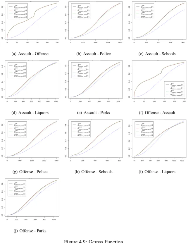
Based on the result obtained in Figure 4.9 we can see that all three estimations for each pair are above the theoretical line (Poisson line). Theoretical is computed assuming CSR which means that results of estimations above the theoretical line mean clustering and esti-mations below Poisson line means repulsion. In our case, in every plot we can observe the estimations above the Poisson line, so every pair of patterns examined show clustering.

Note that this analysis is for homogeneous distribution and not for inhomogeneous, so results can suffer some variations.

(a) Assault - Offense (b) Assault - Police (c) Assault - Schools

(d) Assault - Liquors (e) Assault - Parks (f) Offense - Assault

(g) Offense - Police (h) Offense - Schools (i) Offense - Liquors

(j) Offense - Parks

4.5

Relative Risk

This section is devoted to estimating the spatially-relative frequency of each type of points with respect to each other so that we only apply it to assault-police offices and offense-police offices to see the relative frequency of crimes and offense-police offices.

In relative risk analysis, the aim is to estimate

ρ (u) = λX(u)

λY(u)

, u∈ W, (4.8)

where λX and λY are the intensity functions of point processes X and Y , respectively. For

more details see Kelsall et al. (1995).

In order to estimate the relative risk (4.8), one can use plug-in intensity estimators. However, (Kelsall et al.; 1995; Davies et al.; 2017) recommended using a common band-width for estimating both numerator and denominator. We then used “Hazelton” method, described in Hazelton (2008), which is also implemented in R package “sparr” and function “LSCV.risk”. This function finds the common bandwidth by minimizing a weighted-by-control MISE of the (raw) relative risk function.

As previously mentioned, we have two crime point patterns assault and offense where we are interested in estimating the corresponding relative risk of these two patterns with respect to the pattern of police offices. This can disclose if the distribution of one pattern is affected by another pattern. In the literature, relative risk might also be represented as the logarithm values of (4.8), however, we here only take the fraction of two intensity estimates.

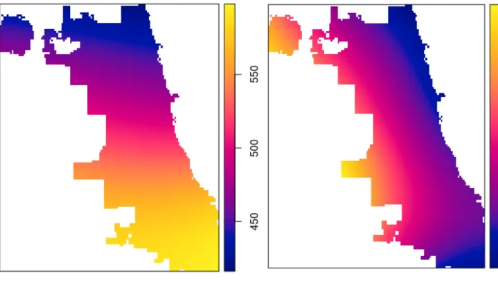
Figure 4.10 (a) shows the relative risk of sex assault crime with respect to police of-fices. For the calculations we have used common bandwidth, calculated using method “Hazelton”, see R package sparr and (Davies et al.; 2017).

We point out that the average relative risk of assault is 505.5217 and for the offense is 403.26. Figure 4.10 confirms that relative risk is not distributed homogeneously. Accord-ing to the Figure 4.10 (a), we can see that the in the South and in the middle of Chicago, the relative risk is higher than the average relative risk. Moreover, Figure 4.10 (b) reveals that the risk in the west of Chicago is higher than the average. The common bandwidth for assault was 15644.24 feet and for offense 15701.79 feet.

(a) Assault (b) Offense

Figure 4.10: Crime relative risk estimations with respect to police offices.

4.6

Distance to Focus

In this section, we build and analyze a model based on the standard method of ecological regression. This method is usually implemented through a mixed effect Poisson log-linear model. In our case we analyzed if the proximity effect to a particular place, in this case parks, can induce more presence of sex-based crimes. The need to combine several inputs of crime events close to the parks using a log-linear formulation is not realistic.

In this case, as proposed by Ramis et al. (2011), we considered the use of a multiplica-tive non-linear distance effect to take into account the underlying spatial structure of the data. We used the model

O_i∼ Po(E_iµi), i= 1, . . . , 98, (4.9) with log{µi} = log{ρ} + 5

∑

Figure 4.11: Focus selected of four neighborhoods in Chicago

i≤ 4. E_istands for the total number of expected cases in each neighborhood under a normal

situation, which is generally estimated by a 2% per tract. The parameter ρ is related to

the overall “sex based crime risk”. The di j stand for the distances between the centroid of

neighborhood i and the focus j. The distances di jare included as a covariate in a continuous

function f (di j; αj, βj) of the form

f(di j; αj, βj) = 1 + αjexp{−(di j/βj)2}, (4.11)

with two parameters, αjaccounting for the elevation in risk at the source, and βjaccounting

for the decay in risk as distance to source increases.

We fitted the model and estimated the parameters of the distance function (See Table

4.1) f (di j), i.e αj, βj, by maximum likelihood. The approximate log-likelihood function,

up to a constant term, is (Diggle et al.; 1997):

L(ρ, θ , α, β ) := −

98

+

98

where µi= ρ 5

∏

To test the hypotheses about the parameters we use the usual generalized likelihood ratio test statistic

D= 2nL( bφ ) − L0( bφ0)

o

, (4.14)

where L0 and L denote the maximized log-likelihoods under the null and alternative

hy-potheses, respectively.

Previous studies have pointed out that the usual asymptotic properties of the likelihood ratio test may not hold for the models considered in this paper because the distance function

is such that when αj= 0, βj is indeterminate. However, following Ramis et al. (2011) this

was solved by assuming that the likelihood ratio test can be considered to have one effective degree of freedom per source, rather than two.

In the context of our application, we considered two tentative models:

1. Null model: µi= ρ, 2. Distance model: µi= ρ 5 ∏ j=1 f(di j),

Model 1 does not take into account any particular spatial structure. Model 2 brings into the model the spatial dependence through a distance function. The selected model based on the full expression in (4.10) is the one that best fits our data.

Table 4.1: Estimation of the distance fucntion parameters

Parameters α β

Focus 1 9.47 95823.47

Focus 2 -0.34 374434.38

Focus 3 3.23 13394.63

Focus 4 1.29 179108.44

We selected four neighborhood trying to cover from north to south all Chicago map. Within each neighborhood, randomly, we selected 4 parks (focus). In table 4.1, we can observe that Focus 2 located on Little Village, is the inhibitor one and Focus 1 in Chatham neighborhood, Focus 3 in Austin and 4 in West Ridge are parks attractors of sex-based

crimes in Chicago. 0 50000 100000 150000 0 2 4 6 8 10 12

Distance function associated to source 1 (ft.)

intensity

0e+00 1e+05 2e+05 3e+05 4e+05 5e+05

−2

−1

0

1

2

Distance function associated to source 2 (ft.)

intensity 0 5000 10000 15000 0 1 2 3 4 5

Distance function associated to source 3 (ft.)

intensity 0 50000 100000 150000 200000 0.0 0.5 1.0 1.5 2.0 2.5 3.0

Distance function associated to source 4 (ft.)

intensity

Figure 4.12: Fitted functions per focus.

We can observe the graphical output for the distance functions, in Figure 4.12, depend-ing on the estimated parameters as given in Table 4.1. We note that all focuses except Focus 2 have a positive value of parameter α indicating that focuses 1, 3 and 4 have an attractive behavior of this type of crime. Focus 2, on the contrary, has a detractor behavior. The value

The larger it is, a smoother decay presents the interaction function. The constant function at 1 indicates the case of no spatial relation among crimes and distance to the focus.

4.7

A first look at the Temporal Analysis

We analyzed the data temporary in a very simply way, separating space from time. We cre-ated some graphs to see how crimes are distributing on time, for example the distribution by year, seasons, months and day of the week.

We can observe in the histograms of Figure 4.13 that Sexual Assault crime (b) is more stable on time and there were not many variations for the last 10 years. For Sex Offense (c) crime we can observe a high drop on crime rates from 2007 to 2017. If we check the Total

Crimeshistogram (a) we can observe in a general view that crime is decreasing slowly.

In the histograms of Figure 4.14, we can see that the months where we can find a peak of crimes are the summer months. We divided the months by seasons; from December to Febrary is winter (1), from March to May is spring (2), from July to August is summer (3), and from September to November is Autumn (4). As we can see there is a peak in the range of summer months. The same happens when we analyze the crimes by month. We can found more crimes occurring on June, July and August (Histogram Figure 4.16).

The last one, is the histogram Figure 4.16, where we analyzed crimes day by day. In the last 10 years, sex-based crimes were more concentrated on weekends (Saturday and Sunday). For Sexual Assault, we can see this concentration clearly on weekends but for Sex Offense seems that there is not a preferred day. We can see a increasing on Tuesday and Thursday. This analysis could give us more information if we obtain the result for each month of the last year and not with a global analysis of 10 years.

(a) Total Crimes per year (b) Sexual Assaults per year

(c) Sex Offenses per year

(a) Total Crimes by Seasons (b) Sexual Assault by Season

(c) Sex Offense by Season

(a) Total Crimes by months (b) Sexual Assault by monnths

(c) Sex Offense by months

(a) Total Crimes per day of Week (b) Sexual Assault per day of Week

(c) Sex Offense per day of Week

Part IV

Conclusions

Chapter 5

Conclusions, Limitations and Future

Lines of research

5.1

Conclusions

In this section, we are going to explain the conclusions and results that we have obtained on the previous analysis. We focused on solving the main objectives and research question of this thesis; 1) if sex-based crime in Chicago has spatial variations, 2) if there is any inter-action between events from the same data pattern and 3) if there is any interinter-action between different types of crimes.

We can see in our results that the distribution of the two point patterns analyzed in the city of Chicago varies spatially. As we can see in Figure 4.2 (a) and (b) they are distributed creating clusters in the space. We also calculated the intensity of Sexual Assault and Sex offense crimes and we can see which parts of the city has more intensity. In the Sexual Assault case, Figure 4.5 (a), we can observe a higher intensity in the middle-south and north-west of Chicago. The intensity of Sex Offense, Figure 4.5 (b), are a bit more spread than Sexual Assault where we can found higher intensity in middle-south, north-west and north-east of Chicago city.

in Figure 4.2 (a) and (b) that both types of crimes have a cluster distribution. Points of the same typology tend to be aggregated in space.

For research question 3, first we analyzed the distances from points of crime type 1 (sexual assault) to points of crime type 2, and we discovered that the maximum distance to find a sex offense from a sexual assault crime was 500 feet (152.4 meters) approximately same distance from offense to assault. To be more concise we apply the Kcross inhom analysis and we found out that sexual assault and sex offense are dependent, what means that the probability of finding one type of crime close to the other type of crime is high. As well the distribution of the crime on space is inhomogeneous and creates clusters in space.

For temporal analysis, we only introduced on the first steps of the analysis. Results are visible on Figures 4.13, 4.14, 4.15 and 4.16. Andresen and Malleson (2015) analyzed the patterns of different types of crimes in Vancouver, Canada. They found patterns for some types of crimes but they could not find any temporal pattern during weekdays on Sexual Assault crime, being a bit higher on Tuesday/Wednesday and Saturday. In our case, the study based on Chicago, we found a clear temporal pattern on Saturday and Sunday. Not occurring the same as Sex Offense crime, where the temporal distribution is more homoge-neous. As we have seen, the offenders also have daily routines and their crimes are modeled on that routines. During weekends, people use to have more free time and less organized activities as during week time (Ceccato; 2011), and also offenders. So, it is more probable that one offender can target a victim.

5.2

Limitations

This subsection is created to explain what limitation we have found in the creation of this thesis and possible future lines of research.

The limitation we have found is about data. Data was downloaded from an open data portal from Chicago, but not all the data were available or updated. One of the data not updated were the population data. Last update was in 2013 about the 2010 year population.

Our analysis was from 2007 to 2017. The population is changing a lot in a year and even more if we need to focus on neighborhood population, which was our case. In this case, we could not find any population per each neighborhood available on data portal.

5.3

Futures Lines of research

This part is created to express future lines of research that we think could be interesting.

Once analyzed all area of Chicago city it would be interesting to select micro-scale areas within Chicago in order to analyze deeply. To know why some neighborhoods have more or fewer crimes than other, to analyze the behavior of crime spatial and temporal dis-tribution on small areas within a neighborhood could give important and extra information about criminal events, as needs or problems in some streets or common areas. That also allows police officers to know better their city and neighborhood and to create strategies to prevent future crimes. As Shiode et al. (2015) found, at micro-scale areas we can found different patterns for the different types of crimes than high areas.

Another interesting future line of research is the temporal analysis. Here we only in-troduced a basic analysis separated from the spatial component because it was not the principal aim of this thesis. One future research could be analyzing temporal patterns, first to differentiating daytime crimes and night crimes and adding the spatial factor to see if the spatial distribution, taking into account some range of hours, months or seasons, create variations or differences. As Cohen and Felson (1979) explained crime can be affected by the daily habits and repetitive daily activities.