Autonomous parking using 3D perception

(1)

Universidade de Aveiro Departamento de Engenharia Mecânica 2012

Joel Filipe Pereira

Estacionamento autónomo usando perceção 3D

(2)

(3)

Universidade de Aveiro Departamento de Engenharia Mecânica 2012

Joel Filipe Pereira

Estacionamento autónomo usando perceção 3D

Autonomous parking using 3D perception

Dissertação apresentada à Universidade de Aveiro para cumprimento dos req-uisitos necessários à obtenção do grau de Mestre em Engenharia Mecânica, realizada sob orientação científica de Vítor Manuel Ferreira dos Santos, Pro-fessor Associado do Departamento de Engenharia Mecânica da Universidade de Aveiro

(4)

(5)

O júri / The jury

Presidente / President Prof. Doutor Jorge Augusto Fernandes Ferreira

Professor Auxiliar da Universidade de Aveiro

Vogais / Committee Prof. Doutor Paulo José Cerqueira Gomes da Costa

Professor Auxiliar da Faculdade de Engenharia da Universidade do Porto

Prof. Doutor Vítor Manuel Ferreira dos Santos

(6)

(7)

Agradecimentos / Acknowledgements

O cumprimento dos objetivos estipulados para este trabalho deve-se, em grande parte, à ajuda e apoio demostrados por algumas pessoas.

Ao Professor Doutor Vítor Santos por ter aceite tão prontamente ser meu ori-entador e por me ter mostrado e encorajado nos novos mundos da perceção 3D.

Aos meus colegas do Laboratório de Automação e Robótica por todo o es-pírito de equipa e boa disposição demonstrada nas longas noites de trabalho. Ao Jorge Almeida pela imensa sabedoria e opiniões fornecidas.

Finalmente, ao Miguel Oliveira, por todo o tempo e paciência depositados no meu trabalho. Miguel, funcionou!

(8)

(9)

Palavras-chave Estacionamento paralelo; Veículo não-holonómico; ROS; Kinect; Trajetórias compostas.

Resumo Este trabalho enquadra-se no contexto da condução autónoma, e o objetivo principal consiste na deteção e realização de uma manobra de estaciona-mento paralelo por parte de um veículo não-holonómico à escala de 1:5, utilizando um ambiente de programação ROS. Numa primeira fase são de-tetados os possíveis lugares vagos com recurso a uma nuvem de pontos proveniente de uma câmara 3D (Kinect), analizando volumes ao lado do carro. Assim que é encontrado um lugar vazio, inicia-se o estudo de pos-síveis trajetórias de aproximação. Estas trajetórias são compostas e são geradas em modo offline. É escolhido o melhor caminho a seguir e, no final, envia-se uma mensagem de comando para o veículo executar a manobra. Os objetivos traçados foram alcançados com sucesso, uma vez que as manobras de estacionamento foram realizadas corretamente nas condições esperadas. Para trabalhos futuros, seria interessante migrar este algoritmo de procura para outros veículos e tipos de manobra.

(10)

(11)

Keywords Parallel parking; Non-holonomic vehicle; ROS; Kinect; Composed trajecto-ries.

Abstract This work fits into the context of autonomous driving, and the main goal consists of the detection and execution of a parallel parking manoeuvre by a 1:5 scaled non-holonomic vehicle, using the ROS programming environment. In a first stage, the possible parking locations are detected by analysing a point cloud provided by a 3D camera (Kinect) and specifically by analysing volumes on the side of the car. Whenever an empty place is found, the study of possible paths of approach begins. These are composed trajectories, being generated offline. The path to follow is evaluated, and then the commands needed to the vehicle perform the selected path are sent. The outlined objec-tives were successfully achieved, since parking manoeuvres were performed correctly in the expected conditions. For future work, it would be interesting to migrate the search algorithm to other types of vehicles and manoeuvring.

(12)

(13)

List of Figures

1.1 Non-holonomic model of a car . . . 6

1.2 First easy parallel parking prototype . . . 7

1.3 Inria auto parking car . . . 7

1.4 Autonomous driving competition track . . . 8

1.5 First atlas robot prototype . . . 8

1.6 Atlas - Autonomous driving competition champions . . . 9

1.7 Atlascar 1 - The first full scale prototype . . . 9

1.8 ROS - simple network of process . . . 10

1.9 Kinect camera for Xbox 360 . . . 11

1.10 Scheme of the programming procedure . . . 12

2.1 Camera information path . . . 13

2.2 Stereo pair of images . . . 14

2.3 Kinect example of depth image . . . 14

2.4 Panasonic D-Imager sensor . . . 15

2.5 Infra-red pattern emitted by the Kinect sensor . . . 15

2.6 LiDAR system . . . 16

2.7 Sick LiDAR system with a rotating axis . . . 17

2.8 Automotive Radar applications . . . 17

2.9 Ultrasonic parking sensors . . . 18

2.10 Operation of the navigation unit . . . 18

2.11 Bosch parking space detector system . . . 19

2.12 Lexus LS460 parking itself . . . 20

3.1 Empty parking spot coordinates . . . 24

3.2 Kinect test of minimum range . . . 25

3.3 Kinect mounting position . . . 25

3.4 Device constructed to accommodate the Kinect sensor . . . 26

3.5 Final assembly of the sensor . . . 27

3.6 Comparison between point cloud XYZRGB and point cloud XYZ . . . 29

3.7 Kinect horizontal field of view . . . 29

3.8 Reconstructed point cloud with odometry information . . . 30

3.9 Points from volume input parameters . . . 31

3.10 Green points inside a convex hull . . . 32

3.11 Points from convex hull coordinates . . . 33

3.12 Hulls of empty parking spot search . . . 35

3.13 Search frames . . . 35 iii

(16)

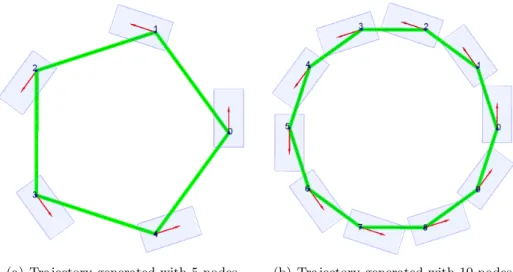
4.3 Circular trajectories generated with different number of nodes (segments) 42

4.4 Geometric parameters of a car-like vehicle . . . 43

4.5 The three different types of Ackerman steering . . . 43

4.6 Example of a set of trajectories - the first planned position is node 0 . . . 45

4.7 Distance to attractor point (DAP) on node 7 = 0 . . . 46

4.8 Angular difference to attractor point (ADAP) . . . 47

4.9 Collision points - yellow cylinders . . . 48

4.10 Chosen trajectory - traj 2 . . . 51

4.11 Speed modulation on forward/reverse movement . . . 52

4.12 Gamepad control buttons . . . 54

4.13 Some of the generated trajectories . . . 55

4.14 Simplified Communication scheme . . . 56

5.1 Straight forward motion to calibrate the odometry . . . 59

5.2 Final odometry calibration . . . 60

5.4 Parking detection - type I . . . 61

5.5 Parking detection - type II . . . 62

5.6 Processing times on trajectories evaluation . . . 62

5.7 AtlasMV Ackeman angle . . . 63

5.8 Circular trajectory planed and executed (lifted up the ground) . . . 63

5.9 Circular trajectory planed and executed (on the floor) . . . 64

5.10 ‘S’ shaped trajectory . . . 64

5.11 Clothoid path . . . 65

5.12 Parking manoeuvre - type I . . . 66

5.13 Parking manoeuvre - type II . . . 66

(17)

List of Tables

1.1 Autonomous cars achievements through the years . . . 5 2.1 Kinect sensor specifications . . . 16 4.1 Trajectory evaluation weights . . . 50

(18)

(19)

Code sections

3.1 Transformation publisher . . . 26

3.2 Kinect point cloud re-publisher . . . 28

3.3 Nodelet launch file . . . 30

3.4 Convex hull extraction . . . 31

3.5 Empty spot detector . . . 32

3.6 Callback function . . . 33

3.7 Recorder launch file . . . 36

3.8 Playback launch file . . . 36

4.1 Frames transformations . . . 44

4.2 Distance to attractor point . . . 46

4.3 Angular difference . . . 47

4.4 Free space . . . 48

4.5 Distance to obstacles . . . 49

4.6 Speed modulator . . . 51

4.7 Command message . . . 52

4.8 Gamepad control message . . . 53

(20)

(21)

Part I

Guidelines

(22)

(23)

Chapter 1

Introduction

It did not take many decades since the mass production of automobiles (1913) for compa-nies to start thinking about autonomous driving. At the Norman Bel Geddes’s Futurama exhibit, sponsored by General Motors at the 1939 World’s Fair, appeared the very first idea of an autonomous vehicle - an electric car, controlled by radio and powered by circuits embedded in the roadway [O’Toole, 2009].

Despite having an early start, the legislation didn’t allow this type of vehicles on pub-lic roads until June of 2011, when the State of Nevada became the only place in the World to authorize the use of autonomous cars on highways [Markoff, 2011]. The approved law defines an autonomous vehicle as “a motor vehicle that uses artificial intelligence, sensors and global positioning system coordinates to drive itself without the active intervention of a human operator” [Nevada, 2011].

As it was forbidden to circulate with autonomous cars on the street, technological developments followed another path - the creation of small driving aids. Nowadays it is clear that there is an increasing use of electronic components in cars, which are intended to improve the safety of vehicle’s occupants. The new trend is to incorporate long-range sensors such as cameras or radars, to improve passengers and other cars safety [Fossati et al., 2011].

1.1 Autonomous cars

In the second half of the twentieth century some research institutions began to develop their prototypes of autonomous vehicles. Some of the most remarkable concepts are presented below.

The first project to achieve success in the development of a driverless vehicle was concluded in 1977 by the Tsukuba Mechanical Engineering Laboratory in Japan. It tracked white street markers (on a clearly marked course) using computer vision and achieved speeds up to 30 km/h. One of the biggest difficulties of that project was the hardware required, since commercial computers were much slower than they are today [Schmidhuber, 2011, Chiafulio, 2010].

In the 1980s Ernst Dickmanns and his group at the University Bundeewehr Munich (UniBW) built robot cars using parallel computers and applying techniques such as saccadic vision (cameras focus on the most relevant points of interest) and probabilistic approaches (use of Kalman filters). They started the project "VaMoRs" equipping a

(24)

Mercedes-Benz van, table 1.1, with cameras and computers to track lane markings of an highway, achieving speeds up to 100 km/h. This application was helped by the strong geometric constraints available from knowledge of highways. Despite doing a safe driving, the initial experiments took place without traffic.

Since 1994 the Robot Car "VaMoRs-P", in short "VaMP" (table 1.1), managed to drive all by itself, at speeds up to 130 km/h. This car was equipped with a range of sensors for autonomous navigation comprising the sense of vision and inertial sensors for accelerations and angular rates. Road and object recognition was performed both in a look-ahead and in a look-back region.

In 1995 Ernst Dickmanns finishes the "VITA-2" project which is a twin car of the "VaMP". They were two autonomous vision based Mercedes 500SL (tracking up to 12 cars) which have driven more than 1000 km on the Paris multi-lane ring reaching speeds of 130 km/h, automatically passing slower cars. One year later, the "VaMP" Mercedes drove from Munich to Copenhagen and back (more than 1600 km) exceeding speeds of 170 km/h and completing the journey with 95% of autonomous driving [Schmidhuber, 2011, Chiafulio, 2010, Aloimonos, 1997].

In 1995 began the ‘No Hands Across America’ project. During this tour of America, which was sponsored by Delco Electronics, AssistWare Technology, and Carnegie Mellon University, two researchers drove more than 4000 km with an autonomous vehicle, the Navlab 5 (table 1.1), which uses video images, to determine the location of the road ahead, and GPS/gyroscope information to estimate the current position. The appropriate steering position was calculated using all the data received from the sensors. One of the project’s limitations was the need to humanly operate the throttle and brake pedals [Schmidhuber, 2011, Chiafulio, 2010, Jochem et al., 1995].

In the late 90s an Italian project (ARGO) modified a car, a Lancia Thema 2000 (ta-ble 1.1), which could follow the white marks in a highway. The vehicle was equipped with two black-and-white video cameras. The images acquired by the cameras were analysed in real-time and the results of the processing were used to drive an actuator mounted onto the steering wheel, which was the only fully autonomous component of the car. However, this car was very important on the path of autonomous driving, because of the use of low-cost components [Schmidhuber, 2011, Chiafulio, 2010, Bertozzi et al., 1998].

The year of 2005 was the debut of the DARPA Grand Challenge, which is “(...) a field test intended to accelerate research and development in autonomous ground vehicles that will help save American lives on the battlefield.” [Darpa, 2007]. The Grand Challenge is not limited to college students. It brings together organizations from the industry to backyard inventors who are looking for a technological challenge. The course took place in the desert and had a large amount of GPS points to follow [Schmidhuber, 2011, Chiafulio, 2010]. The large majority of participants used new forms of perception of the external environment, such as LiDAR systems, which can provide a very accurate 3D map of the surrounding region. The winner of the competition was the ‘Stanley’ car (table 1.1) from the Stanford University.

In 2006 began the ELROB (European Land Robot Trial) which is not a competition, but a pure demonstration of what European robotics is able to achieve today. The EL-ROB is an annual event and alternates between a military and a civilian focus each year. This competition brings great benefits to the development of algorithms for navigation and perception, because the circuits have obstacles that were not known initially (the track is maintained secret until the day of the event) [Schmidhuber, 2011, Chiafulio, 2010,

(25)

1.Introduction 5

Schneider, 2012].

The DARPA Challenge returned in 2007 now with the name of “DARPA Urban Challenge”. This time the autonomous vehicles must run trough an urban environment respecting traffic signals. The competition was won by Carnegie Mellon University (ta-ble 1.1).The sensors began to be more elegant, and some of the semi-autonomous vehicle characteristics started to be included by some motor companies like Audi, Volvo and GM. [Schmidhuber, 2011, Chiafulio, 2010].

Table 1.1: Autonomous cars achievements through the years

Year Project Achievement Image

1980s VaMoRs Track road markers on highway [VaMoRs, 2012]

1994 VaMoRs-P Road and objects recognition [Behringer, 2007]

1995 Navlab 5

4000 km with autonomous

[NavLab, 2012] steering-wheel control

1998 Argo

Autonomous driving using

[Vislab, 2009] low-cost components

2005 Stanley Champion of the 1st Darpa event [Hudson, 2008]

2007 Tartan Champion of the Urban Darpa [Tartan, 2012]

2010 Google car First legal autonomous car [Ackerman, 2010]

(26)

Most recently Google showed the world its vision of what an autonomous car is (table 1.1). They took a normal Toyota Prius and assemble on it a LiDAR sensor (a Velodyne), some radars, a camera, a GPS and IMU, and a speed encoder fixed to the rear wheel. They manage to navigate autonomously in several occasions, using the maps provided by Google maps. Nowadays, this car is the only one in the World which is legal to be autonomously driven, in the State of Nevada.

1.2 The parking manoeuvre

Over the years, the growth of metropolitan areas has led to an exponential increase on the number of cars and consequently to a decrease on the available parking spaces.

From all the types of parking manoeuvres, parallel parking is the one that best optimizes the available space on the street, but also the most difficult to achieve. Driving forward into a parking space on the side of a road is usually not possible. The driver should reverse into the spot to take advantage of a single empty space.

Because of all of that, the parking manoeuvre is something that worries many people, not only for its complexity but also for the need to be done quickly to prevent the formation of traffic jams. The car is the principal responsible for this complexity because it is a non-holomic system (figure 1.1) where the number of control commands available is less than the number of coordinates that represents its position and orientation. Here the final state of the system depends on the intermediate values of its trajectory through the space. So, there are positions which are reachable by holonomic systems, but which are not achievable by non-holonomic ones in the presence of obstacles.

Figure 1.1: Non-holonomic model of a car

In 1934 was presented the first prototype of a vehicle with an easy parallel parking system (figure 1.2). That model consisted on the raise of the vehicle with four hy-draulic jacks with wheels that allowed the car to move sideways to fit on the available space. Despite the great technological advance presented this model was never produced [Brown, 1934].

(27)

1.Introduction 7

Figure 1.2: First easy parallel parking prototype [Brown, 1934]

The first vehicle to be able to do a parallel parking without human intervention was developed at INRIA (Inventeurs du monde numérique, France) in the 90s. The car was an electric Ligier model equipped with sonars at the front and rear bumpers to measure distances (figure 1.3). It was possible to drive the car until the appearance of a row of parked cars. Then, the turn of a switch put the car in automatic mode making it move forward and looking for empty spaces with the help of the sonars. If a spot is found, a computer calculates all the distances required and send information to the electric motors (engine and steering wheel) to perform the manoeuvres. This project allows the car to leave the parking lot automatically too, but all the movements were limited to flat ground [INRIA, 1998].

In 2000 this project was extended to the perpendicular parking manoeuvre, but the car employed a LiDAR system to sense the surrounding space.

Figure 1.3: Inria auto parking car [Paromtchik, 2012]

Nowadays, car brands have been investing large amounts of money to develop elec-tronic components to aid the driver in parking manoeuvres. Systems that go from the parking spot detection to the most advanced ones that control the steering wheel on the parking manoeuvre have been released in the past few years.

(28)

1.3 The ATLAS project

The ATLAS project begun in 2003 in the group of Automation and Robotics from the Department of Mechanical Engineering of the University of Aveiro. The main goal of the project was the development of advance sensing and active systems to implement in mobile robots which were created to participate at Autonomous Driving competition (AD) taking place at Portuguese Robotics Open [FNR, 2012].

The AD represents a technical challenge, in which autonomous robots must travel along a road like scenario, which is composed of several visual patterns (figure 1.4). This contest is divided in 3 stages, of increasing complexity. The fastest robot to complete the course is the winner. Time penalties are given when robots run of the road, bump into obstacles or disrespect traffic signs.

Figure 1.4: Autonomous driving competition track

The first robot of the Atlas series (figure 1.5) was based on an aluminium frame with two wood layers. It has a mechanical differential to provide traction and only one webcam looking at a v-shape mirror to allow the entire visualization of the sides of the road.

(29)

1.Introduction 9

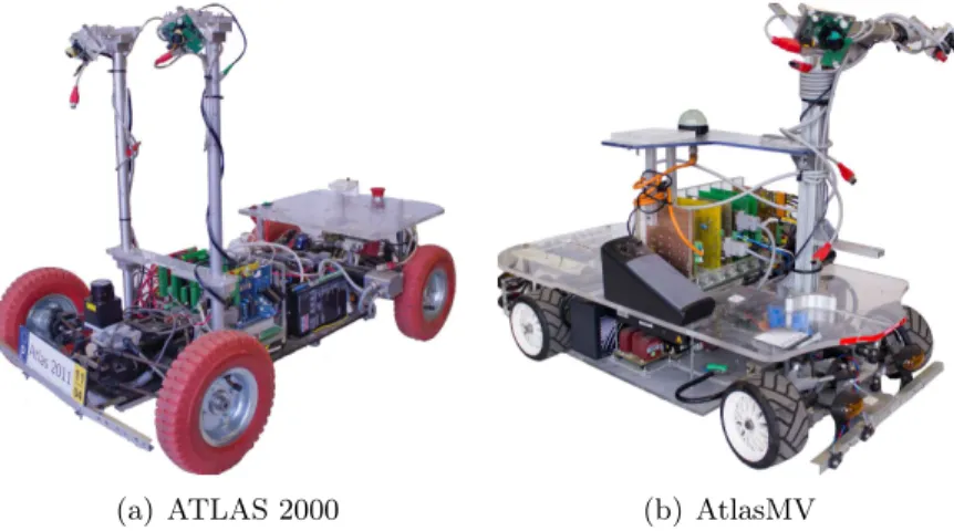
The next prototype to be made was the ATLAS 2000 (figure 1.6(a)) a 1:4 scale model used by model makers to achieve a similar relation to a common car. In 2006 the ATLAS team won for the first time the AD competition with this car, repeating the victory in 2007. Several upgrades were carried out to obtain better performances from the robot.

In 2008 a new robot was developed, the AtlasMV (figure 1.6(b)), to improve the performances of its predecessor. That robot was designed to be smaller (1:5), lighter and faster. New steering control mechanisms, pneumatic braking systems (later replaced by hydraulic brakes) and active perception unit were developed.

(a) ATLAS 2000 (b) AtlasMV

Figure 1.6: Autonomous driving competition champions

Nowadays the Atlas group is evolving to deal with real road scenarios. To achieve this objective, a full sized prototype (1998 Ford Escort), the ATLASCAR 1 (figure 1.7), was equipped with several state of the art equipment. A 200A alternator, a 3000W inverter, lasers sensors, a stereo camera, a IMU, a GPS, among others [ATLAS, 2011, Santos et al., 2010].

(a) Atlascar 1 front-view (b) Atlascar 1 rear-view

Figure 1.7: Atlascar 1 - The first full scale prototype [ATLAS, 2011]

1.4 The Robot Operating System

“ROS (Robot Operating System) provides libraries and tools to help software developers create robot applications [ROS, 2012]”.

(30)

It provides services that are available on an operating system such as hardware ab-straction, low-level device control functionality and message passing and packages man-agement.

To fully understand the ROS philosophy it should be noted that it has three levels of concepts. The filesystem, the computation graph and the community.

The filesystem is composed by the resources found on disk, such as:

• Packages - the unit of ROS organization. They may contain ROS runtime processes (nodes), libraries, data-sets, etc.

• Manifests - provide information about a package, like the library dependencies and compiler flags.

• Stacks - a collection of packages.

• Message types - define data structures to the messages sent in ROS.

The computation graph (figure 1.8) represents the network of ROS processes. There are a few computation concepts:

• Nodes - as ROS is designed to be modular, nodes are processes that perform com-putation.

• Master - it provides names registrations and lookup for the rest of computation graphs.

• Messages - are a simple data structure which allows communication between nodes. • Topic - is the name used to identify the concept of the message.

• Bags - are the format to save and playback ROS messages data.

ROS Topic

node node

Package

Service invocation

Subscription Publication

Figure 1.8: ROS - simple network of process

The ROS community allows the exchange of stacks, packages and knowledge between the global users.

These characteristics turn ROS into a good platform to develop code. However, ROS currently only runs on Unix-based platforms.

(31)

1.Introduction 11

1.5 Objectives

Due to the great importance that has been given to the autonomous parking, the primary objective of this thesis is on the programming and implementation of that manoeuvre into an autonomous driving vehicle, the ATLASCAR 1.

Conducting a parking manoeuvre requires making two fundamental tasks, the first is the search for an empty space where to park the car and the second one consists of the approach to the required final position of the vehicle.

1.5.1 Parking spot detection

To begin the search for a parking place, it is very important to know first what can be considered an empty spot. Humans encounter locations to park the car in many different situations. However, it is very difficult to ‘tell’ a machine what are all the parking possibilities, since they are endless. So, this thesis must cover only the most difficult parking manoeuvre, which is the parallel one (due to the non-holonomic nature of the vehicle).

The information about the surrounding environment should be given by a Kinect®

sensor (figure 1.9) not only because it is a new type of hardware present on the laboratory, but also because of the huge acceptance that this sensor has taken on the researchers community and the big precision/price ratio.

Figure 1.9: Kinect® _{camera for Xbox 360}

The selection of the parking space must be variable in accordance to the vehicle dimensions and mechanical restrictions keeping always in mind that the robot is a non-holonomic vehicle in a world with some obstacles and traffic rules.

One last thing to have in mind, is that another project related to the ATLASCAR prototype is being developed to allow the automatic actuation of the gearbox (once the original car transmission is manual), so it may be necessary to operate another navigation robot of the laboratory (e.g. the AtlasMV) on a smaller scale scenario.

1.5.2 Planning the parking manoeuvre

After the parking spot has been detected and selected, an algorithm must generate some approaching trajectories to achieve the desired coordinates and orientation. Those tra-jectories must assume a complex form, which means that the vehicle may change its turning angle while moving forward or backwards.

(32)

The choice of one trajectory to follow should be studied in another algorithm because of the importance to complete the manoeuvre without collisions and by the shortest path, always having in consideration the non-holonomic nature of the model.

After all, and if the program assumes that there is an empty spot which is reachable, a message should be sent to the low level controls of the robot so it can follow the programmed path.

Summing up, the entire process can be outlined by the scheme presented in figure 1.10.

3D sensor (Kinect) Point Cloud treatment Empty spot detection Propose multiple paths Choose one path Send control message to the robot Spot detection _manoeuvreApproach

Figure 1.10: Scheme of the programming procedure

1.5.3 ROS utilization

This thesis must be done using the ROS environment not only because of all the li-braries, drivers and packages existing, but also because the Laboratory of Automation and Robotics was at the time migrating all of its code to that platform. All of the work should be done not only to satisfy a single task, but also to be useful to the community of researchers of the laboratory.

(33)

Chapter 2

State of the Art

2.1 Perception of the external environment

Since its emergence, autonomous vehicles make use of perception systems. The sur-rounding environment and the state of the car are sensed by the use of techniques such as computer vision, LiDAR, radar or GPS/INS.

2.1.1 Computer Vision

“The goal of computer vision is to make useful decisions about real physical objects and scenes based on sensed images [Shapiro and Stockman, 2000]”.

Many of the activities performed by human beings in day-to-day would not be possible without the use of vision, so it becomes clear why the first prototypes of autonomous driving cars used computer vision to detect obstacles and the road.

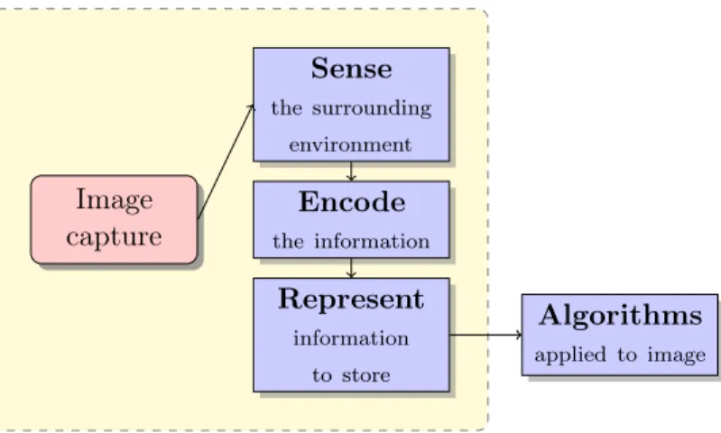
From the camera, with the information gathered, there is a path to follow, as shown in figure 2.1. Image capture Sense the surrounding environment Encode the information Represent information to store Algorithms applied to image

Figure 2.1: Camera information path

One of the techniques applied on autonomous vehicles consists of the use of a stereo camera (or two cameras) which generates a stereo pair of images (figure 2.2). In those

(34)

two images it is possible to identify pairs of corresponding points. Those points allow the calculation of the distance between the projected point in the three-dimensional world and the recording cameras [Klette and Liu, 2008].

(a) Left (b) Right

Figure 2.2: Stereo pair of images [Klette and Liu, 2008]

Another technique consists of the analysis of a video sequence (multiple frames). Motion estimation for these sequences should provide information about movements of objects for each sequence, identifying possible conflict paths. By applying several filters (such as Canny edge detector) to the image sequence it becomes possible to identify obstacles and the road in different positions through the time. This allows the creation of a vector with speed and trajectory to each object identified [Klette and Liu, 2008].

2.1.2 3D image cameras

3D image cameras work much like an ordinary camera to capture the two dimensions of an image. To add the third dimension (which gives the depth information of the scene, figure 2.3) there are two different methods which can be used. The time of flight imaging (ToF) and the structured light imaging.

Figure 2.3: Kinect example of depth image

The ToF technique consists of measuring the depth of a scene quantifying the changes that the emitted light encounters. It can be divided in two different principals:

(35)

2.State of the Art 15

• Pulsed modulation - Measures distances to objects by measuring the total time that a light pulse needs to travel to an obstacle and bounce back.

• Continuous wave modulation - Measures distances evaluating the phase of the wave reflected from the obstacles encountered.

One example of a sensor which works with the ToF principals is the D-Imager (fig-ure 2.4) which was announced by Panasonic in 2010.

Figure 2.4: Panasonic D-Imager sensor [Koifman, nd]

On the other hand, the structured light imaging technique consists of the projection of a known light pattern to the scene. The distortion provoked on the patern will give the information about the distances, figure 2.5.

Figure 2.5: Infra-red pattern emitted by the Kinect sensor [Fisher, 2012]

The Kinect, figure 1.9, which was first announced on June of 2009 under the code name “Project Natal”, is currently the most popular of this kind of systems because of its low price and the open nature of the communication code. The sensor specifications are presented in table 2.1.

(36)

Table 2.1: Kinect sensor specifications

Field of view Data stream Range

Horizontal Vertical Depth RGB min-max 57◦

43◦ 320×240 640×480

0.6-8.0 m 30 Hz 30 Hz

2.1.3 LiDAR Sensors

LiDAR - Light Detection And Ranging - (also known as LADAR) is a technology that can measure distances to objects using infrared, visible or ultraviolet light. This technology has several decades, yet its commercial application have only been developing in recent years.

In this system the higher the power of the light beam the greater is the achievable range. However, this system should compromise the power of the laser to prevent injury to the eyes of people who may be affected [Schwarz, 2010]. Also, LiDAR has some problems with certain weather conditions because it uses a form of light, which is easily reflected, dispersed, and sometimes absorbed by rain or fog, resulting in loss of information.

The basic elements of a LIDAR system (figure 2.6) are a laser scanner, a rotating mirror and a cooling system. The scanner is designed to record the time that the laser pulse takes to be reflected and return since it was emitted. The rotating mirror causes the laser beam to disperse through an angle which allows the construction of a 2D map. By adding another degree of freedom (e.g. rotation axis, figure 2.7) to the LiDAR sys-tem, it becomes possible to obtain a three dimensional representation of the surrounding environment.

(a) LiDAR System components (b) LiDAR sensor - Sick S3000 [Sick, 2012]

(37)

Figure 2.7: Sick LiDAR system with a rotating axis [Matos, 2003]

2.1.4 Radars

Today, some cars are equipped with sensors that measure the distance up to other vehicles or large objects in front of them.

Automotive radar sensors are less expensive and still offer the advantages of microwave-based sensing with respect to laser sensors and video cameras [Rohling, 2008].

There are two primary methods of measuring distances using radar:

• Direct propagation - consists of the measurement of the delay associated with the emission and reception of the signal. This delay is function of the speed of radio waves and its period.

• Indirect propagation - also known as FMCW (Frequency Modulated Continuous Wave), consists of the emission of a modulated frequency. The difference between the emitted and received frequency can be used to directly determine the distance as well as the relative speed of the object.

The main applications for the automotive radars can be divided in three main groups, as shown in figure 2.8.

Radar

Comfort Control Safety

Figure 2.8: Automotive Radar applications

• Comfort - This area is ensured by parking aid sensors (which avoid the need of drilling holes in the bumpers) and blind spot warning system.

• Control - The active cruise control (ACC) is similar to a regular cruise control, but it verifies if there is any slower car in front of the vehicle, and regulates the travelling speed.

(38)

• Safety - If the radar sensors detect an eminent collision (Closing Velocity Sensing) a signal is sent to the vehicle control system to deploy some safety features (like the seat belt pre-tensioners).

2.1.5 Ultrasonic Sensors

Ultrasound is an acoustic wave with a frequency beyond human hearing (more than 20 kHz) and its propagation speed (approximately 340 m/s) is slower than light or radio waves, which allows measurements using low speed signal processing.

Ultrasonic sensors are used to determine the distance or direction of an object from the time the waveform takes to make a round trip to the target. The range of a sensor of this type is much smaller than that of a LiDAR system, so their use is greater in short-range applications, such as in parking assistance systems (figure 2.9). In these systems, sensors in the front and rear bumpers emit ultrasonic signals that are reflected by an obstacle in the range of detection. Traces of the reflected ultrasound are received by the sensors and their travel time is measured, calculating then the distance to the obstacle [Hikita, 2010].

Figure 2.9: Ultrasonic parking sensors [Hikita, 2010]

2.1.6 GPS and INS

Driverless vehicles require a very precise information about its position, so they use a system which works similarly to the scheme shown in figure 2.10.

Navigation Unit

GPS INS

GPS data loss INS growing errors

(39)

Most navigation systems, these days, depend on the availability of information from their GPS coordinates to estimate the position of the vehicle. GPS satellites transmit information to receivers and, through the use of triangulation, the exact position of the user is estimated. Despite being very accurate, it is common that the GPS information is not reliable, because there can be loss of data (in tunnels or near high buildings). To overcome this loss of signal is used a INS (Inertial Navigation System) which uses accelerometers and gyroscopes to check changes in the position of the vehicle at a certain period of time. However, the GPS is very useful to correct the growing errors of the INS. So, both sensors can work in a single way, but their results are better if working together [Baker et al., 2006].

2.2 Autonomous parking

In recent times there have been many brands of automobiles that released to the market mechanisms to help the parking manoeuvre, since the technology is still expensive and not very reliable and the law does not allow fully autonomous parking.

It began with the use of ultrasonic sensors which detected the proximity of vehicles from the front and rear bumpers of the car which was performing the parking manoeuvre. Later, ultrasonic sensors that warned the driver if there was a parking space big enough to perform the manoeuvre safely were introduced (figure 2.11). After the intro-duction of this system appeared a mechanism that gave the driver the instructions about the direction that the steering-wheel should have at every moment. In vehicles which have electric powered direction, the steering-wheel may even be controlled independently, letting the driver control only the pedals.

Figure 2.11: Bosch parking space detector system [Bosch, 2011]

These systems are virtually equal in all vehicles, being the Lexus LS460 (figure 2.12) the first production vehicle to be presented with a semi-autonomous parking system (the Lexus Park Assist). After this one, car brands like Toyota, Mercedes, Ford among others, presented their own solution (all of them very similar).

(40)

Figure 2.12: Lexus LS460 parking itself [AutomotiveAdicts, 2006]

All systems developed to date have encountered problems when the car does not meet the pre-programmed situations. For example, when there is a car parked in second row, or when there are pedestrians near the side-walk.

The need for perfect conditions make it nearly impossible to have a reliable self-parking system.

(41)

Part II

Methods and Programming

(42)

(43)

Chapter 3

Parking spot detection

Humans look for an empty parking space with a certain logic and criteria which is hard to ‘teach’ to a machine. So, in order to programme an autonomous parking spot detector, some simplifications should be done. This part of the thesis will describe the paths followed to allow the search for open spaces to park a robotic car. Some of the code made for this purpose will appear in a yellow shaded rectangle with an explanation at the bottom.

3.1 Analysis of the parking spot and vehicle

3.1.1 Parking spot definition

The first thing to be done when developing a parking spot detector algorithm is the definition of what a parking space is. There are several types of parking situations, like parallel, perpendicular, angled, among others. From all the kinds of manoeuvres the most difficult one to be done quickly and in safe conditions (due to the non-holonomic characteristics of car-like vehicles) is the parallel parking.

For those reasons, the chosen parking approach method to be done autonomously is the parallel manoeuvre.

3.1.2 Used vehicle

As explained on section 1.5.1, the work developed on this thesis must be inserted on the Atlascar global project. However, the vehicle used on that project was not ready (until the present date) to operate the gear box autonomously, so it became necessary to apply the parking algorithm to a robotic vehicle available at the laboratory, the AtlasMV, which is a 1:5 scale model of a road vehicle.

The code developed should be generic enough to allow its use on different kind of vehicles with simple and quick modifications. Due to that, the migration of the code to a full scale model (the Atlascar) should be pretty easy and will be explained in each part of the code.

3.1.3 Search method

The surrounding environment is perceived by a point cloud which, in this case, is gen-erated by a Kinect sensor. The parking space coordinates (figure 3.1) are obtained by

(44)

treating the information which comes from the cloud generated.

Figure 3.1: Empty parking spot coordinates

To this type of parking space there is only one limitation: the parking spot must be always preceded by another parked car (or object). This is due to the fact that it is very difficult for a machine to realise what a parking space is. So, on the search zone, the algorithm only considers a parking space if there is another vehicle behind that place.

3.2 Point cloud reconstruction

In order to reconstruct the external environment it was necessary to build some hardware and code a few ROS packages. Those processes are explained on the following subsections.

3.2.1 Kinect assembly

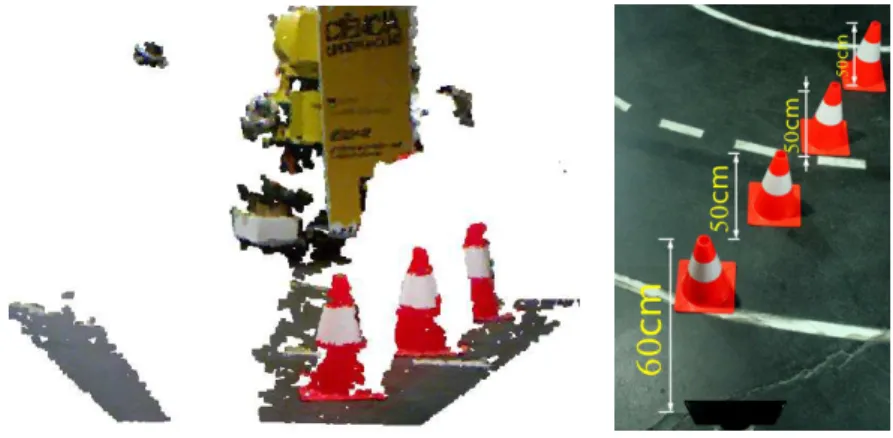
The Kinect sensor was not built to operate in outdoor conditions, since when it is exposed to direct sunlight the infrared sensor becomes saturated. As consequence, there is no information about the depth of the scene exposed. Due to that, the use of the Kinect sensor on the Atlascar vehicle will be very limited. Only in low light conditions (e.g. cloudy weather or at night) this sensor will provide an accurate point cloud information. However, the navigation should not be limited by the weather, so in non favourable conditions to the Kinect, the point cloud should be provided by another sensor, like the stereo camera or lasers.

The AtlasMV vehicle is an indoor robot, so the use of the Kinect is perfectly allowed. To receive the point cloud provided by this sensor it was used an existent driver on the ROS repository, the openni_kinect.

As it was said on section 2.1, this camera has a range of 0.6 to 8.0 meters when measuring the depth of a scene. In figure 3.2 it can be seen that the closest cone to the camera is not perceived by the depth sensor and it generates a lack of information projection shadow.

(45)

3.Parking spot detection 25

(a) Point cloud minimum range limitation (b) Top view of mini-mum range test

Figure 3.2: Kinect test of minimum range

In order to maximize the use of the optimal range of the camera and to allow the search for parking spaces at a reduced distance from the line of parked cars, the Kinect was mounted on the right side of the vehicle and facing the left side (figure 3.3). So, the parking manoeuvre performed by this vehicle will be done following the left side of the road and not the right, like most of the countries legislation assumes.

Figure 3.3: Kinect mounting position

Because of the chosen mounting position and the limited field of view of the camera there would be hidden point cloud information. To overcome that loss, an adjustable mounting device was built. This device can be regulated in height and in two different angles (figure 3.4) in order not only to make the parking spot search more accurate, but also to allow different utilizations of the sensor in future works.

(46)

(a) Kinect support (b) Rear view of the mounted support

Figure 3.4: Device constructed to accommodate the Kinect sensor

After the Kinect assembly on the mounting device and posterior fixation to the At-lasMV robot, it was needed to define the position of the camera frame in relation to the one of the car. It was made by a ROS node which is responsible to publish the transformation between frames.

Code section 3.1: Transformation publisher

#i n c l u d e <r o s / r o s . h>

#i n c l u d e < t f / t r a n s f o r m _ b r o a d c a s t e r . h>

#i n c l u d e <std_msgs / F l o a t 6 4 . h>

#i n c l u d e <math . h>

i n t m a i n(i n t argc, char∗∗ argv ) {

ros: : init ( argc , argv , " pub_ trans f or m at i o ns ") ; ros: : NodeHandle n ;

tf: : TransformBroadcaster broadcaster ;

ros: : Rate r ( 1 0 ) ;

f l o a t a l p h a= ( 3 8 . 0 ) ∗( M_PI /180) ;// the a n g l e o f the camera

tf: : Transform transform ( btMatrix3x3 (0 , − 1 , 0 , cos ( alpha ) , 0 , sin ( alpha ) , −sin ( ←֓ a l p h a) , 0 , cos ( alpha ) ) ,

b t V e c t o r 3( 0 . 2 3 6 , −0.05 , 0 . 6 8 ) ) ;

w h i l e( n . ok ( ) ) {

b r o a d c a s t e r. sendTransform ( tf : : StampedTransform ( transform , ros : : Time : : now ( ) ←֓ ," / vehi cl e_ odom etry ", " / openni_camera ") ) ;

r. sleep ( ) ; ros: : spinOnce ( ) ; }

}

The first thing which is done in this piece of code is the variable initialization. The ROS node is called pub_transformations, and there is a broadcaster of transformations called broadcaster.

After the determination of the tilt angle of the camera, which may be done using the ROS package kinect_aux, the transformation matrices were defined. The matrices

(47)

correspondent to the rotation (equation 3.1) and distances between frames (equation 3.2) are calculated by replacing the values of the angles and distances in the correspondent place.

Rot =  

cos θ − sin θ cos α sin θ sin α sin θ cos θ cos α − cos θ sin α

0 sin α cos α   (3.1) ∆r =   ∆x ∆y ∆z   (3.2)

In the present case (figure 3.5), the matrices parameters are: • θ = −π/2 rad

• α = (38.0) ∗ (π/180) rad • ∆x = 0.236 m

• ∆y = −0.05 m • ∆z = 0.68 m

Figure 3.5: Final assembly of the sensor

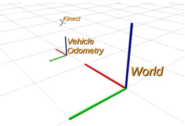
After the definition of the transformation to broadcast (named transform), composed by a 3×3 rotation matrix and a 3×1 ∆r vector, a while loop start to broadcast the trans-formation between the vehicle_odometry (center of the rear axle) and the openni_camera (center of the kinect sensor) frames. The last two lines of cycle are responsible to keep the loop at a rate of 10 Hz.

(48)

To migrate this piece of code to the Atlascar vehicle the only part which needs to be changed is the transformation matrix that should assume values measured after the kinect assembly on the car.

3.2.2 Frequency modulator

The openni_kinect package available on ROS repository publishes the point cloud infor-mation at a relatively high rate. Later this became undesirable when other process were in execution in the same processor. So another node was created, responsible to receive the point clouds from the openni_kinect and publish them back, but at a slower rate.

Code section 3.2: Kinect point cloud re-publisher

( . . . )

v o i d c o n v e r s i o n (c o n s t s e n s o r _ m s g s: : PointCloud2ConstPtr & pcmsg_in ) {

pcl: : PointCloud<pcl : : PointXYZ> pc_cut ; pcl: : PointCloud<pcl : : PointXYZ> processed_pc ; s e n s o r _ m s g s: : PointCloud2 pcmsg_out ;

pcl: : fromROSMsg (∗ pcmsg_in , pc_cut ) ;

p c _ c u t. header . frame_id=pcmsg_in−>header . frame_id ;

f o r (i n t i=0; i<(i n t) pc_cut . points . size ( ) ; i++) {

i f ( pc_cut . points [ i ] . z >0.6 && pc_cut . points [ i ] . z < 1. 5) p r o c e s s e d _ p c. push_back ( pc_cut . points [ i ] ) ;

}

p r o c e s s e d _ p c. header . frame_id=pc_cut . header . frame_id ; pcl: : toROSMsg ( processed_pc , pcmsg_out ) ;

p c m s g _ o u t. header . stamp=pcmsg_in−>header . stamp ; c l o u d _ p u b. publish ( pcmsg_out ) ;

}

i n t m a i n(i n t argc, char ∗∗ argv ) {

ros: : init ( argc , argv , " kinect_freq_mod") ; ros: : NodeHandle n ;

ros: : Rate loop_rate ( 1 0 ) ; ( . . . )

// S u b s c r i b e o f the K i nect p o i n t c l o u d message

ros: : Subscriber sub = n . subscribe (" / point_cloud_ from _kinect ", 1 , conversion ) ;

// A d v e r t i s e o f the r e s u t a n t p o i n t c l o u d

c l o u d _ p u b = n . advertise<sensor_msgs : : PointCloud2 >(" / poi nt_ cl oud_ i nput", 1) ;

w h i l e( ros : : ok ( ) ) { ros: : spinOnce ( ) ; l o o p _ r a t e. sleep ( ) ; } r e t u r n 0 ; }

At the main function, this code subscribes a point cloud from the Kinect, and executes a callback each time a message is received. The callback is responsible to reduce the amount of points existent in the original point cloud. This is achieved by confining the depth information of the message. In this case, only the points which are between 0.6 and 1.5 meters in the depth axis are considered acceptable, since the other points do not bring any additional information to the parking spot localization.

(49)

In the “while” cycle the new point cloud is published at a rate defined by the ros::Rate, which in this case is 10 Hz.

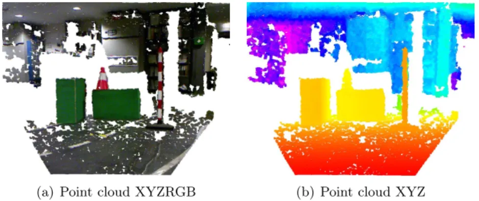
To reduce even more the size of the message transmitted, only the geometric parame-ters of the point cloud (x, y and z) are sent. The Kinect also provides colour information about the scene, but to detect volumes it is not necessary (figure 3.6).

(a) Point cloud XYZRGB (b) Point cloud XYZ

Figure 3.6: Comparison between point cloud XYZRGB and point cloud XYZ To migrate this code to another vehicle, the only thing which needs changes is the callback. There, the distances which limits the depth of the point cloud are optimized to the use on the AtlasMV vehicle. New values should be defined to use on another vehicle.

3.2.3 Point cloud accumulator

The Kinect horizontal field of view does not allow the search for an empty parking space at the normal search distance (figure 3.7). To overcome this limitation there were two possible solutions. The first one consisted of a search for a parking space made at a bigger distance, however this may be impossible due to the traffic regulations restrictions. The other solution assumed a reconstruction of the point cloud (figure 3.8). To proceed to the reconstructions the only two things that are needed are the point cloud and the odometry information of the vehicle (the vehicle position on the global frame at each time).

Figure 3.7: Kinect horizontal field of view

(50)

Figure 3.8: Reconstructed point cloud with odometry information

There was already a C++ class developed in the Laboratory of Automation and Robotics server which was responsible to accumulate points to a certain frame of accu-mulation. To use that class it was just necessary to include the node on the launch file (file which manages the processes to launch).

Code section 3.3: Nodelet launch file

<launch> ( . . . )

</node> </launch>

In the pc_accumulation node there are some parameters which need to be defined. • “distance_from” - means the distance accumulated in meters.

• “time_value” - is the period of the message.

• “acc_frame” - is the accumulation frame (where the point cloud must be recon-structed).

• “removed_from” - is the frame of the odometry message.

This node also provides a tool which can reduce the point cloud density of the resul-tant accumulated point cloud, the voxel_size. In this case, a voxel grid of 0.03 meters means that each point is separated from the others by at least 0.03 meters.

The parameters that mandatorily need to be changed when migrating the code are the odometry message, the frame of accumulation and the accumulated distance.

3.3 Volume detection

The volume detection is made by the use of functions which provide informations about the presence or not of points at a certain zone. All the processes and code are shown in

(51)

the next subsections.

3.3.1 Points from volume extraction

To verify if there were any points from a point cloud at a certain region of space it was created a C++ class which, with some input parameters, determines the existence or non-existence of points. That class assumes that the input parameters (figure 3.9) are:

• Convex hull point cloud - Those points (at least three) define the geometric figure of the solid which will be extruded. This solid is in fact the region of search for points.

• Positive/negative offset - It defines the height of the extruded solid. The positive offset indicates the amount of positive extrusion, and the negative do the opposite. • Zone flag - This flag is very important because it establishes if the search zone is

inside the convex hull (negative flag) or outside it (positive flag).

Figure 3.9: Points from volume input parameters

Code section 3.4: Convex hull extraction

( . . . )

pcl: : ExtractPolygonalPrismData<T> epp ; ( . . . )

pcl: : ExtractIndices <T> extract ; // C r e a t e s the e x t r a c t i o n o b j e c t

pcl: : PointIndices : : Ptr indices ; i n d i c e s. reset ( ) ;

i n d i c e s = pcl : : PointIndices : : Ptr (new pcl: : PointIndices ) ; ( . . . )

i f ( (i n t) indices −>indices . size ( ) !=0) {

e x t r a c t. setInputCloud ( pc_in . makeShared ( ) ) ; e x t r a c t. setIndices ( indices ) ;

e x t r a c t. setNegative ( flag_in_out ) ; e x t r a c t. filter ( pc_in_volume ) ; }

( . . . )

(52)

On the C++ class code it is defined a polygonal prism data of extraction (epp) which is responsible to verify if the points from the point cloud in study are inside or outside the limits of search. The indices of the points which satisfies the condition are returned and indicate the points from the point cloud which are in the required area.

One of the public parameters of the class which may be obtained is a point cloud containing only the points inside (or outside if pretended) the defined convex hull (fig-ure 3.10).

Figure 3.10: Green points inside a convex hull

3.3.2 Empty volume detection

This is the section responsible for the main execution of the package “parking_detection”, which looks for empty volumes at a certain search zone. Thanks to the classes and execution nodes that were previously made, the main goal of this executer is to make all the nodes work together.

Code section 3.5: Empty spot detector

i n t m a i n(i n t argc, char ∗∗ argv ) {

( . . . )

tf: : TransformListener listener ( n , ros : : Duration ( 1 0 ) ) ; ( . . . )

P u b l i s h e r = n . advertise<trajectory_planner : : coordinates >(" / m s g_ coordi nates ", ←֓ 1000) ; // ______________________ // |_______Markers________| c a r _ p u b = n . advertise<visualization_msgs : : Marker >( " c a r ", 0 ) ; ( . . . ) // ______________________ // | _____ConvexHulls______ | // ConvexHull 1

c o n v e x _ h u l l 1. header . frame_id="/ vehi cl e_ odom etry "; pcl: : PointXYZ pt1 ;

pt1. x = spot_length /2 + spot_length / 2 ; pt1 . y= ( spot_wide + spot_distance ) + ←֓

s p o t _ w i d e/ 2 ; pt1 . z= 0 . 0 2 ; c o n v e x _ h u l l 1. points . push_back ( pt1 ) ; ( . . . ) pfv. set_convex_hull ( convex_hull1 ) ; ( . . . ) // ______________________ // | ______PointCloud______ | // P oi nt Cloud p u b l i c a t i o n s

(53)

( . . . )

// ______________________ // |______PCL s u b s c r ._____|

// C r e a t e s a ROS s u b s c r i b e r f o r the i n p u t p o i n t c l o u d

ros: : Subscriber sub = n . subscribe ("/ pc_out_pointcloud ", 1 , cloud_cb ) ; ros: : Rate loop_rate ( 3 0 ) ;

ros: : spin ( ) ; }

Initially a listener is defined and will wait for transformations information between frames. After that it is important to initialize a publisher, which will be very useful later to send the parking coordinates message.

There are other publishers defined to represent markers (objects drawn on rviz, which is a visualizer from ROS). The coordinates that will define the vertices of the figure to extrude into a convex hull are also initialized in this section of code. These points are geometrically defined by the position of the convex hull vertices in relation of the search vehicle (figure 3.11).

Figure 3.11: Points from convex hull coordinates

At the end, the point clouds resultant from the class “points_from_volume” appli-cation are published. One of the last parameters is a subscriber, which runs a callback function every time a message of type “pc_out_pointcloud” is received.

Part of the code present in the callback is shown bellow.

Code section 3.6: Callback function

#d e f i n e VEHICLE_FRAME " / vehi cl e_ odom etry "

v o i d c l o u d _ c b (c o n s t s e n s o r _ m s g s: : PointCloud2ConstPtr & pcmsg_in ) {

// STEP 1 : C reate the poi nt_ cl oud i n p u t

(54)

pcl: : PointCloud<pcl : : PointXYZ> pc_in ; pcl: : fromROSMsg (∗ pcmsg_in , pc_in ) ;

//STEP 2 : Query f o r the t r a n s f o r m a t i o n to us e

tf: : StampedTransform transform ;

( . . . )

p _ l i s t e n e r −>lookupTransform ( pcmsg_in−>header . frame_id , VEHICLE_FRAME , ←֓ ros: : Time ( 0 ) , transform ) ;

( . . . )

//STEP3 : t r a n s f o r m pc_in u s i n g the q u e r i e d t r a n s f o r m

pcl: : PointCloud<pcl : : PointXYZ> pc_transformed ;

pcl: : PointCloud<pcl : : PointXYZ> pc_ahead , pc_spot , pc_behind , pc_ground ; p c l _ r o s: : transformPointCloud ( pc_in , pc_transformed , transform . inverse ( ) ) ; p c _ t r a n s f o r m e d. header . frame_id = VEHICLE_FRAME ;

// STEP 4 : A pl yi ng the ConvexHull c l a s s

pfv. convexhull_function ( pc_transformed , 0 . 0 , −0.6 , f a l s e) ; p c _ a h e a d=pfv . get_pc_in_volume ( ) ;

p c _ a h e a d. header . frame_id = VEHICLE_FRAME ; ( . . . )

// STEP 5 : Convert to ROSMsg

s e n s o r _ m s g s: : PointCloud2 pcmsg_out ; pcl: : toROSMsg ( pc_ahead , pcmsg_out ) ;

( . . . )

// STEP 6 : Markers

v i s u a l i z a t i o n _ m s g s: : Marker marker_car ;

m a r k e r _ c a r. header . frame_id = VEHICLE_FRAME ;// Frame name

( . . . )

m a r k e r _ c a r. type = visualization_msgs : : Marker : : CUBE ;// Marker type

m a r k e r _ c a r. pose . position . x = 0 . 8 / 2 ; m a r k e r _ c a r. pose . position . y = 0 ;

m a r k e r _ c a r. pose . position . z = spot_high / 2 ; ( . . . )

// STEP 7 : P u b l i s h markers and PClouds

c a r _ p u b. publish ( marker_car ) ; ( . . . )

c l o u d _ p u b. publish ( pcmsg_out ) ; ( . . . )

}

There is a transformation applied to the point cloud in order to draw the points on the “world” frame. After that, the class “points_from _volume” which verifies if there are points inside a certain volume is executed. The returned point cloud is converted into a ROS message to be published later. This callback is also responsible for the construction of the markers which represents the convex hulls latter published.

To migrate the code to another vehicle, the changes to apply are only in the dimen-sions of the convex hull (they must respect the new vehicle geometry), and the size of markers, which are a representation of the convex hulls. The “_VEHICLE_FRAME_” should be also the same of the one published by the vehicle low level.

3.3.3 Parking coordinates message

As soon as some conditions are met, a message with the parking spot coordinates (po-sition and orientation) is send to the trajectory planner module. The conditions (fig-ure 3.12) necessary to assume that there is a parking space are indicated on the following items.

(55)

Figure 3.12: Hulls of empty parking spot search

• Parking behind convex hull - This convex hull should have points in it, because it was assumed that to found an empty parking space it is necessary first to find an occupied zone.

• Parking space convex hull - As expected there is a zone were no points should exist. This zone will be the parking space.

• Floor convex hull - This complementary zone determines if the ground has a certain amount of points, because if there are holes on the ground the parking manoeuvre may be very dangerous.

If the conditions are respected, a position message is sent.

This message contains information about the geometric position of the parking spot and the orientation on the base frame - world (figure 3.13).

Figure 3.13: Search frames

(56)

3.4 Possibilities of package launch

One of the advantages of ROS utilization is the possibility to organize the code in nodes and create “launch files” which just execute some of the nodes.

In the case of the parking spot detection this may be very useful, because of the possibility of replay some recorded situations.

3.4.1 Record data

The launch file ‘parking_detection_bagrecord.launch’ has the responsibility of launch the necessary nodes to record a ‘bagfile’ which contain the reconstructed point cloud and the transformations between all the frames.

Code section 3.7: Recorder launch file

<node name=" openni_node " pkg=" openni_camera " t y p e=" openni_node "/> ( . . . )

( . . . ) </node>

</launch>

3.4.2 Playback mode

If there is any bagfile stored on disk (just bagfiles recorded with the necessary informa-tion), the launcher ‘parking_detection_bagplay.launch’ may be executed. This will treat all the incoming data, as if it were happening at the moment. However, it will be just a playback action.

To publish the recorded information there is a ROS node which must be used, the ‘rosbag play’.

Code section 3.8: Playback launch file

<launch> <node name=" p a r k i n g _ d e t e c t i o n " pkg=" p a r k i n g _ d e t e c t i o n " t y p e=" p a r k i n g _ d e t e c t i o n " ←֓ /> <param n a m e=" /use_sim_time " t y p e=" b o o l " v a l u e=" t r u e " /> </launch> 3.4.3 Live action

The last launch file is the one responsible to perform live action. It is very similar to the launcher used to record the information. However, on this one there is no need to launch the last node which was only responsible to record the selected information. The

(57)

‘parking_detection.launch’ launcher is the one to be used when executing the complete parking manoeuvre (search, plan and execution).

(58)

(59)

Chapter 4

Planning a manoeuvre

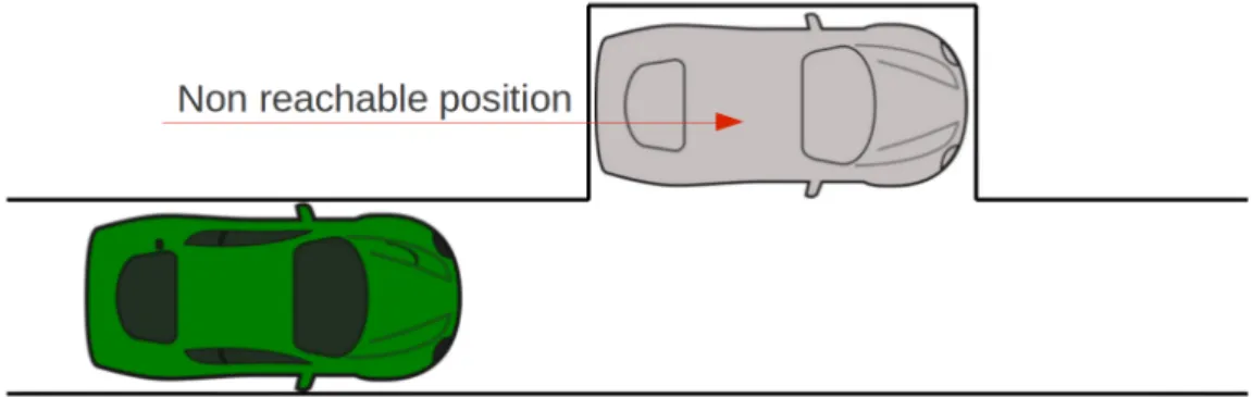
Planing a non-holonomic vehicle trajectory is harder than planning for an holonomic one. This kind of mobile robots, by not being able to rotate around themselves, have positions in space that are simply not achievable (figure 4.1). So, in order to plan a manoeuvre, it is necessary to use some method which define the path for a car-like vehicle.

Figure 4.1: Non reachable position to a non-holonomic vehicle

4.1 Planning approaches

The very first ideas of path planning were published in the first International Joint Conferences on Artificial Intelligence (late 60s). Nowadays there are three main families of methods to find out the better path to follow; the ‘roadmap’, the ‘cell decomposition’ and the ‘potential field’ approaches [Laumond et al., 1997, Latombe, 1990].

4.1.1 Roadmap

A roadmap is composed by lines of free space which a robotic vehicle may follow between obstacles (figure 4.2).

(60)

Figure 4.2: Example of roadmap navigation lines [Morales, nd]

As soon as the roadmap is obtained, it is necessary to identify three different paths: • 1 - From the starting point up to some point on the roadmap;

• 2 - A continuous roadmap path;

• 3 - From the roadmap up to the desired final point.

If these paths exist and are continuous, then there is a path from the initial until the goal point. The principles to the roadmap creation may lay on different techniques, such as visibility graphs, voronoi diagrams, freeway net and silhouette [Latombe, 1990].

4.1.2 Cell decomposition

This method consists of the sub-sampling of the navigation space in small cells, forming the nodes of a connectivity graph. Two nodes are said connected if the cells which represent them are adjacent to each other.

The path (channel) to follow is defined, if there are adjacent cells from the starting point up to the goal point. An optimization algorithm is responsible to ensure that the best possible channel is found [Latombe, 1990, Lingelbach, 2004].

4.1.3 Potential field

The potential fields are obtained by dividing the navigation scene in a small grid, and then calculating the forces applied on the vehicle. Usually, the navigation robot is reduced to a single point and subject to the attraction or repulsion fields. The presence of obstacles will generate repulsion forces on the vehicle, while the goal point produces an attractive field to the robot. The resultant ‘virtual’ force is responsible to conduct the movement of the robot.

Despite being very efficient when compared to other methods, this technique may lead into a non return situation if a local minima is achieved [Latombe, 1990].