Microgrid architecture evaluation for small and medium size industries

(1)

Escola Superior de Tecnologia de Tomar

Filipe Alexandre Guido Bandeiras

MICROGRID ARCHITECTURE EVALUATION

FOR SMALL AND MEDIUM SIZE INDUSTRIES

Dissertação de Mestrado

Mestrado em Engenharia Eletrotécnica Especialização em Controlo e Eletrónica Industrial

(2)

(3)

Escola Superior de Tecnologia de Tomar

Filipe Alexandre Guido Bandeiras

MICROGRID ARCHITECTURE EVALUATION

FOR SMALL AND MEDIUM SIZE INDUSTRIES

Dissertação de Mestrado

Orientado por:

Prof. Mário Gomes – IPT/ESTT Prof. Paulo Coelho – IPT/ESTT

Dissertação apresentada ao Instituto Politécnico de Tomar para o cumprimento dos requisitos necessários à obtenção do grau de Mestre em Engenharia Eletrotécnica –

(4)

(5)

This work was partially supported by the Portuguese Foundation for Science and Technology (FCT) and by PIDDAC, under the research project INDuGRID –

(6)

(7)

ABSTRACT

Industrial customers are looking for ways to reduce their energy consumption and carbon footprint through energy efficiency measures and clean energy sources such as solar and wind power generation systems. In contrast to large industrial enterprises, it may be difficult for smaller industries to improve their energy efficiency due to limited financial conditions and lack of awareness towards cost-efficient applications of renewable energy sources. Nevertheless, the increased integration of clean energy sources in the industrial sector turned microgrids into an important asset to help mitigate the environmental impact from the use of fossil fuels for power generation. Microgrids contribute to a significant increase in reliability and quality to the supplied power without any disturbances and interruptions. These benefits can only be assured by a protection system capable of operating effectively during any abnormal condition.

This dissertation addresses several aspects aiming to assist in the study of industrial microgrid architectures. This work presents an overview of the most common communication technologies and energy sources for microgrids, as well as control strategies for power converters and other control aspects such as droop control method and hierarchical control. In addition, it also addresses several protection methods that can be implemented in microgrids, including protection devices and earthing schemes commonly adopted in low voltage distribution systems. Finally, a case study is presented in order to observe how a centralized and decentralized deployment of energy sources affects the performance of a small industrial microgrid in different scenarios and fault events.

Keywords: Industrial microgrid, centralized/decentralized architecture, renewable energy

sources, energy efficiency, communication technologies, control strategies, protection system, distribution system

(8)

(9)

RESUMO

Os clientes industriais procuram formas de reduzir o consumo energético e a sua pegada ecológica através de medidas de eficiência energética e fontes de energia limpa, como sistemas de geração de energia solar e eólica. Contrariamente às grandes empresas industriais, pode ser difícil para as pequenas indústrias melhorar a sua eficiência energética devido a condições financeiras limitadas e à falta de consciencialização para as aplicações económicas das fontes de energia renováveis. No entanto, o aumento da integração de fontes de energia limpas no setor industrial fez com que as microrredes se tornassem uma mais valia para atenuar o impacto ambiental associado ao uso de combustíveis fósseis para geração de energia. As microrredes contribuem para um aumento significativo de fiabilidade e qualidade da energia fornecida sem quaisquer distúrbios e interrupções. Estes benefícios só podem ser assegurados com um sistema de proteção que seja capaz de operar efetivamente durante qualquer condição anormal.

Esta dissertação aborda vários aspetos que visam auxiliar no estudo de arquiteturas de microrredes industriais. Este trabalho apresenta uma visão geral das tecnologias de comunicação e fontes de energia mais comuns para microrredes, assim como estratégias de controlo para conversores de potência e outros aspectos de controlo, como o método de droop control e o controlo hierárquico. Além disso, são também abordados vários métodos de proteção que podem ser implementados em microrredes, incluindo dispositivos de proteção e esquemas de ligação à terra frequentemente usados em sistemas de distribuição de baixa tensão. Finalmente, é apresentado um estudo de caso para observar como uma implementação centralizada e descentralizada de fontes de energia afeta o desempenho de uma pequena microrrede industrial em diferentes cenários e eventos de falha.

Palavras-chave: Microrrede industrial, arquitetura centralizada/descentralizada, fontes de

energia renováveis, eficiência energética, tecnologias de comunicação, estratégias de controlo, sistema de proteção, sistema de distribuição

(10)

(11)

ACKNOWLEDGMENTS

First and foremost, I would like to express my sincere gratitude to professor José Fernandes and my advisors Mário Gomes and Paulo Coelho for all the help and guidance with the research and writing of this work. Their continuous support and knowledge were essential throughout the development of the project report that served as baseline to this dissertation and two papers. These papers were later submitted to a conference held in France and granted my first experience as presenter.

Finally, I wish to thank my parents and grandparents for providing me with encouragement throughout my whole life and to my closest friends and colleagues for supporting me during my studies and development of this work.

This work was partially supported by the Portuguese Foundation for Science and Technology (FCT) and by PIDDAC, under the research project INDuGRID – Efficient energy management in industrial microgrids with high penetration of PV technology, Ref.: ERANETLAC/0006/2014.

(12)

(13)

4.3.1. Modbus ... 26 4.3.2. DNP3 ... 26 4.3.3. IEC 61850 ... 27 5. Microgrid architecture ... 29 5.1. Distributed generation ... 30 5.1.1. Photovoltaic ... 30 5.1.2. Wind turbine ... 34 5.1.3. Fuel cell ... 36 5.1.4. Micro turbine ... 38 5.2. Energy storage ... 39 5.2.1. Battery storage ... 40 5.2.2. Flywheel ... 41 5.2.3. Supercapacitors ... 43

(15)

6. Power conversion ... 47

6.1. Converter control strategies ... 48

6.1.1. Master-slave control ... 48

6.1.2. Multi-master control ... 49

7. Microgrid protection ... 51

7.1. Feeder protection ... 54

7.2. Bus protection ... 56

7.3. Distributed generation protection ... 56

7.4. Earthing system ... 57 8. Case study ... 61 8.1. Centralized MG ... 64 8.1.1. Case 1C ... 65 8.1.2. Case 2C ... 67 8.1.3. Case 3C ... 69 8.1.4. Case 4C ... 71 8.1.5. Case 5C ... 73 8.2. Decentralized MG... 75 8.2.1. Case 1D ... 77 8.2.2. Case 2D ... 80 8.2.3. Case 3D ... 82 8.2.4. Case 4D ... 84 8.2.5. Case 5D ... 87 8.3. Fault analysis ... 89 8.3.1. Short-circuit analysis ... 91 8.4. Comments ... 92

(16)

xiv

9. Conclusions ... 95

References ... 99

Appendix ... 109

Appendix A – Table of DER technologies ... 109

(17)

LIST OF FIGURES

Figure 1 – Main barriers to energy efficiency in SMEs ... 5

Figure 2 – Concept diagram of a MG [18] ... 9

Figure 3 – Control architecture of a MG ... 11

Figure 4 – Power flow in a transmission line ... 12

Figure 5 – Frequency and voltage droop control characteristic plots... 14

Figure 6 – Basic microgrid architecture ... 29

Figure 7 – Types of solar cell modules [39]: a) Monocrystalline and b) Polycrystalline ... 33

Figure 8 – PV systems: a) Fixed [42] and b) Solar tracker [43] ... 34

Figure 9 – Types of WT technologies: a) VAWT [45] and b) HAWT [46]... 35

Figure 10 – 20 kW SOFC from Wärtsilä [49] ... 37

Figure 11 – 200 kW MT module from Capstone [53] ... 39

Figure 12 – Battery bank [55] ... 41

Figure 13 – Sectional view of a FW system from Beacon Power [60] ... 42

Figure 14 – 56V SC modules from Maxwell: a) Storage bank [62] and b) Single module [63] ... 43

Figure 15 – Master-slave approach (current sources – red and voltage source – green) ... 49

Figure 16 – Multi-master approach (current sources – red and voltage sources – green) ... 50

Figure 17 – Requirement for feeders, buses and generation units... 53

(18)

xvi

Figure 19 – Differential bus protection ... 56

Figure 20 – TT earthing system protection ... 57

Figure 21 – IT earthing system protection ... 58

Figure 22 – TN-C earthing system protection ... 58

Figure 23 – TN-S earthing system protection ... 59

Figure 24 – TN-C-S earthing system protection ... 59

Figure 25 – Electrical schematic of the industrial site ... 62

Figure 26 – Schematic of the MG with centralized generation ... 65

Figure 27 – Bus voltage profile in scenario 1 with centralized generation ... 66

Figure 28 – Bus voltage angle in scenario 1 with centralized generation ... 67

Figure 37 – Schematic of the MG with decentralized generation ... 77

Figure 38 – Bus voltage profile in scenario 1 with decentralized generation ... 79

Figure 39 – Bus voltage angle in scenario 1 with decentralized generation ... 79

(19)

Figure 48 – Centralized MG with internal faults F1 and F2 ... 89

Figure 49 – Decentralized MG with internal faults F1 and F2 ... 90

(20)

(21)

LIST OF TABLES

Table I – European Commission definition of SMEs ... 4

Table II – Main differences between MG and VPP ... 10

Table III – Hierarchical control levels ... 15

Table IV – Wireless technologies characteristics [29, 30] ... 20

Table V – Wired technologies characteristics [29, 30] ... 23

Table VI – TCP/IP model layers ... 26

Table VII – Distributed generation units [36] ... 30

Table VIII – Solar modules efficiencies [38] ... 31

Table IX – Trina Solar modules comparison [39] ... 32

Table X – Small wind turbine characteristics [44, 47, 48] ... 36

Table XI – Fuel cell characteristics [50, 51, 52] ... 37

Table XII – Microturbine characteristics [54] ... 39

Table XIII – Storage units [36] ... 40

Table XIV – Battery storage characteristics [56, 57, 58] ... 41

Table XV – Flywheel characteristics [57, 58, 61] ... 42

Table XVI – Supercapacitor characteristics [57, 58, 61] ... 44

Table XVII – Classification of power converters [68] ... 47

Table XVIII – Protection devices ... 52

Table XIX – Comparison between protection schemes [78, 79] ... 54

Table XX – Load data ... 61

(22)

xx

Table XXII – Network generator data ... 63

Table XXIII – Network bus data ... 63

Table XXIV – Branch data ... 64

Table XXV – Network generator data ... 66

Table XXVI – Network bus data ... 66

Table XXVII – Network generator data ... 68

Table XXVIII – Network bus data ... 68

Table XXIX – Network generator data ... 70

Table XXX – Network bus data ... 70

Table XXXI – Network generator data ... 72

Table XXXII – Network bus data ... 72

Table XXXIII – Network generator data ... 74

Table XXXIV – Network bus data ... 74

Table XXXV – Cable data ... 76

Table XXXVI – Generator group data ... 76

Table XXXVII – Network generator data ... 78

Table XXXVIII – Network bus data ... 78

Table XXXIX – Network generator data ... 80

Table XL – Network bus data ... 80

Table XLI – Network generator data ... 82

Table XLII – Network bus data ... 83

Table XLIII – Network generator data ... 85

Table XLIV – Network bus data ... 85

Table XLV – Network generator data ... 87

(23)

Table XLVII – Fault current results (Amp): Symmetric (3Ph) and Asymmetric

(1Ph) ... 91

(24)

(25)

ACRONYMS AND ABBREVIATIONS

AC Alternating Current

ADSL Asymmetric Digital Subscriber Line

AMR Automatic Meter Reading

ANSI American National Standards Institute

AON Active Optical Network

BB-PLC Broadband Power Line Communication

BS Battery Storage

CHP Combined Heat and Power

CPP Critical-peak Pricing

DC Direct Current

DER Distributed Energy Resource

DG Distributed Generation

DMS Distribution Management System

DNP Distributed Network Protocol

DSL Digital Subscriber Line

DSO Distribution System Operator

ESCO Energy Service Company

FC Fuel Cell

FERC Federal Regulatory Commission

FW Flywheel

(26)

xxiv

GOOSE Generic Object Oriented Substation Event

HAWT Horizontal Axis Wind Turbine

HDSL High-bit-rate Digital Subscriber Line

HTTP Hypertext Transfer Protocol

HV High Voltage

IEC International Electrotechnical Commission

IED Intelligent Electronic Device

IP Internet Protocol

LC Load Controller

LOS Line-of-sight

LV Low Voltage

MC Microsource Controller

MCFC Molten Carbonate Fuel Cell

MG Microgrid

MGCC Microgrid Central Controller

MH Micro Hydro

MMS Manufacturing Message Specification

MPPT Maximum Power Point Tracking

MT Micro Turbine

MV Medium Voltage

NB-PLC Narrowband Power Line Communication

NLOS Non-line-of-sight

NTP Network Timing Protocol

PAFC Phosphoric Acid Fuel Cell

(27)

PEMFC Proton Exchange Membrane Fuel Cell

PEN Protective Earth Neutral

PHS Pumped Hydro Storage

PLC Power Line Communication

PON Passive Optical Network

PV Photovoltaic

RES Renewable Energy Source

RTP Real-time Pricing

RTU Remote Terminal Unit

SC Supercapacitor

SCADA Supervisory Control and Data Acquisition

SME Small and Medium-sized Enterprise

SMV Sampled Measured Values

SOFC Solid Oxide Fuel Cell

SSH Secure Shell

STC Standard Test Conditions

TCP Transmission Control Protocol

TOU Time-of-use

UDP User Datagram Protocol

VAWT Vertical Axis Wind Turbine

VDSL Very-high-bit-rate Digital Subscriber Line

VPP Virtual Power Plant

WLAN Wireless Local Area Network

WPAN Wireless Personal Area Network

(28)

(29)

SYMBOLS AND UNITS

A Ampere

Btu British Thermal Unit

cm Centimetre

ºC Degree Celsius

deg Degree

E Power Converter Voltage

F Frequency

Gbps Gigabit Per Second

GHz Gigahertz

I Current

K Gain

kbps Kilobit Per Second

Kg Kilogram

kHz Kilohertz

km Kilometre

kP Droop Control Frequency Setting

kQ Droop Control Voltage Setting

kV Kilovolt

kVA Kilovolt-ampere

kVAr Kilovolt-ampere Reactive

(30)

xxviii kWh Kilowatt-hour

kWp Kilowatt-peak

m Meter

Mbps Megabit Per Second

MHz Megahertz

mm Millimetres

MVA Megavolt-ampere

MVAr Megavolt-ampere Reactive

MW Megawatt MWh Megawatt-hour P Active Power pu Per-unit Q Reactive Power R Resistance S Apparent Power V Volt V Voltage W Watt Wh Watt-hour Wp Watt-peak X Reactance Z Impedance

δ Power Converter Voltage Angle Δf Frequency Correction Parameter ΔV Voltage Correction Parameter

(31)

θ Voltage Angle

(32)

(33)

1. INTRODUCTION

During the past decades there has been an important development in power systems as a result of an efficient planning and growth in innovation, which led to a considerable quality improvement to the supplied electricity. Nevertheless, the improved quality of the power system is not yet present in every location. Isolated and remote locations still have a defective and faulty power grid with constant power outages. During a power outage of the public power grid, customers may have to wait for days before being reconnected to the power grid and industries that operate with crucial loads cannot afford any power interruption. A failure in the power supply may lead to significant technical problems, production and financial losses [1]. With the integration of distributed generation (DG) into the grid, the reliability and safety of the electric power system became major concerns across the industry, but it also brought the opportunity to include renewable energy sources (RES) and smart control strategies for crucial load supplying in the event of power outages. The environmental concerns associated with power generation from fossil fuels are encouraging industrial customers to look for an alternative clean energy source. This led to the opportunity of considering renewable solutions, such as solar and wind power generation systems. The photovoltaic (PV) systems went through a fast growth in the last decade and these systems are generally characterized by high installation costs, but low operation costs [2]. In addition, there has been a decrease in the module prices of PV systems and the power generation coincides with the peak energy demand during the day [3]. Such systems are an appropriate option for an efficient, reliable and clean industrial power generation system.

This work consists of several chapters addressing different aspects to assist in the study of industrial microgrids. This first chapter briefly introduced a few concerns about the quality of the supplied energy and power outages in the industrial sector, more specifically in isolated and remote locations. It also addressed the fast growth of clean energy sources in power systems due to environmental concerns and decrease in prices. Chapter 2 presents a brief overview of the industrial sector and small and medium-sized enterprises, as well as

(34)

2

their energy consumption and barriers to implement energy efficiency measures, along with the benefits of an efficient energy management and demand response measures in the industry. Chapter 3 introduces the definition of microgrid and how it differs from a conventional passive grid, along with the control architecture and other control aspects such as the droop control method and hierarchical control. Chapter 4 addresses the communication architecture of a microgrid and overviews different communication technologies and protocols that can be implemented in microgrids. Chapter 5 presents a simple architecture of a microgrid to introduce different technologies for generation and storage units, including typical installation costs, efficiency and power rates. Chapter 6 addresses the power converters classification according to their operation in a microgrid, along with an overview of control strategies for power converters. Chapter 7 introduces several microgrid protection strategies and devices adopted to protect feeders, buses and energy resources, as well as an overview of the earthing systems commonly used in low voltage distribution networks. Chapter 8 presents the case study of a small scale industrial microgrid in order to observe how a centralized and decentralized deployment of generation units affects the performance of the microgrid in different scenarios and fault events. Chapter 9 is a conclusion to this work and concludes which architecture configuration is the best fitting for small industrial microgrids, based on aspects addressed in the previous sections.

(35)

2. OVERVIEW OF THE INDUSTRIAL SECTOR

The industrial sector has the highest delivered energy consumption rates among all sectors. As reported in [4], this sector consumes around 54% of the total delivered energy in the world. The industrial sector can be categorized into three distinct categories according to the energy intensity of each industry type. Industries can be classified as energy intensive manufacturing, non-energy intensive manufacturing and non-manufacturing.

The manufacturing industries such as pulp and paper, iron and steel, non-metallic minerals, non-ferrous metals, basic chemicals, petroleum refineries, food and beverage are classified as energy intensive industries. Together, these count for about half of all industrial sector energy consumption. Manufacturing industries that include printing, pharmaceutical products, specialty chemicals and consumer chemicals, as well as fabricated metal products, computer, electronic and optical products, electrical equipment and machinery are classified as non-energy intensive industries. All industries that include activities such as agriculture, forestry, fishing, mining and construction are classified as non-manufacturing industries [5]. Industrial sector energy consumption varies by region and country, according to differences in industrial gross output, energy intensity and the composition of industries. Energy intensity is measured as final energy consumed per unit of gross output [4].

2.1. Small and medium-sized enterprises

According to [5], small and medium-sized enterprises (SMEs) can be defined as non-substantial and independent companies that employ less than a certain number of employees. Depending on this number, enterprises can be classified into micro, small and medium sized enterprises. The criteria for defining the size of an enterprise may differ across countries and it is also dependent on the company annual turnover or balance sheet total. The European Commission defines an upper limit of 250 employees and an annual turnover up to 50 million euro or a balance sheet total below 43 million euro for

(36)

medium-MICROGRID ARCHITECTURE EVALUATION FOR SMALL AND MEDIUM SIZE INDUSTRIES

4

sized enterprises. This limit varies from 20 employees in New Zealand to 1000 employees in China. A SME in Australia has up to 200 employees and the United States considers SMEs up to 500 employees [7]. Table I shows the categories that define SMEs, according to the European Commission.

Table I – European Commission definition of SMEs

Category Employees Turnover (€) Balance sheet total (€) Micro 1 – 10 < 2 million < 2 million

Small 11 – 50 < 10 million < 10 million

Medium 51 – 250 < 50 million < 43 million

The EU recommendation 2003/361 states that SMEs represent 90% of all the businesses in the European Union. Globally, SMEs represent around 99% of all enterprises and provide around 60% of employment. It is known that energy efficiency improvements are typically more cost-effective in all commercial and industrial SMEs, because most of these enterprises have not yet taken advantage of energy efficiency programs that have already been implemented in the larger sectors. As well as energy cost savings and long run positive earnings, energy efficiency improvements may also help mitigate risks when implemented in SMEs. Due to their limited financial condition, SMEs are more vulnerable to market prices increases than larger scale enterprises. At the same time, most SMEs are sensible to power supply disruptions and outages, given their lack of back-up energy systems and on-site generation. Energy efficiency improvements may help reducing these risks, improve energy quality and increase profitability in SMEs [7]. However, smaller enterprises with limited resources and financial conditions may not be capable of implementing energy efficiency programs. Nonetheless, these energy savings can be achieved simply by adopting no-cost and low-cost measures to help reducing energy waste. In the United Kingdom, it is estimated that 40% of the energy savings implemented in SMEs are achieved with minimal financial investment support [8]. Manufacturing SMEs have the highest energy consumption rates among all SMEs. In the United States, the energy demand of manufacturing SMEs is about 50% of the total energy consumed by

(37)

industry. In Italy, manufacturing SMEs energy consumption is about 70% of the total industrial energy demand. Energy demand of manufacturing SMEs in China is estimated to be almost 2.5 times more than the energy demand of large manufacturing enterprises [7].

2.2. Efficient energy management

As previously mentioned in section 2.1, it may be difficult for some SMEs to adopt energy efficiency measures in order to reduce their carbon footprint and energy consumption. Smaller enterprises are unaware of energy efficiency improvements and cost-efficient applications of RES. Lack of motivation and information, as well as no qualified personnel and limited financial conditions are the main barriers to implementing energy efficiency measures in SMEs [9]. Moreover, banks often refuse to engage with small enterprises, because of their lack of collateral to provide an alternative repayment and the high transaction cost of small loans [7].

Figure 1 – Main barriers to energy efficiency in SMEs

Energy efficiency improvements in the industrial sector can go from simple no-cost and low-cost measures to large investments such as RES and the integration of smart grids. The no-cost and low-cost measures can be as straightforward as turning off lights and equipment when not in use, fixing sources of energy losses such as leaks or acquiring energy efficient equipment.

(38)

6

An efficient energy management provides an increase in disposable income and improvements in productivity and air quality. It is an effort to reduce the greenhouse gas (GHG) emissions in the industry and combat the climate change, being the largest contribution to GHG abatement with 49% of the savings projected for 2030 [10]. The increased deployment of low-carbon technologies in the industrial sector has been an important asset to mitigate the environmental impact from the use of fossil fuels for power generation. Altogether, the low-carbon technologies account for almost 25% of the primary energy demand projected for 2030, according to the INDC scenario [10]. This rapidly growth of low-carbon technologies is a result of energy policies and incentives implemented towards the use of RES and other low-carbon options.

2.3. Demand response

According to the definition proposed by the Federal Regulatory Commission (FERC), demand response allows customers to intentionally change their energy consumption or load patterns in response to energy prices over time and incentive payments to induce lower energy usage during certain time periods [11]. Demand response is often used to smooth the energy consumption profiles by shifting the load demand between time periods in order to reduce the energy consumption during critical peak periods. Due to this load shifting from demand response measures, potential stresses on the transmission and distribution grid can also be substantially reduced. Industrial customers implement demand response measures to adjust their production processes according to the energy prices, and thus reducing the costs of the energy consumed. Commercial and residential customers often use automated solutions to manage their energy consumption to reduce energy costs. Implementing demand response measures may bring numerous benefits, including economic efficiency, system reliability and environmental benefits associated with the integration of RES [11]. Demand response can be categorized as price-based or incentive-based depending on the encouragement received to implement demand response measures [12].

 Price-based demand response denotes a response to changes in energy usage by customers according to changes in the market prices they pay. This type of response includes methods such as real-time pricing (RTP), critical-peak pricing

(39)

(CPP) and time-of-use (TOU) pricing. Customers can adjust their energy consumption and load patterns in response to different time periods of electricity prices, reducing their electricity bill by taking advantage of lower price time periods [13].

 Incentive-based demand response denotes measures and programs established by the utility that specify a baseline level of energy consumption during certain time periods. These programs provide load reduction incentives for customers, including direct load control, interruptible and curtailable service, demand bidding and buyback programs, emergency demand response programs, capacity market programs and ancillary services market programs. Customers may be penalized if they fail to reduce their energy consumption according to the demand response program they chose to enrol [13].

(40)

(41)

3. CONCEPT OF MICROGRID

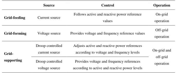
A microgrid (MG) can be seen as an integration of microgeneration, storage units and controllable loads located in a local distribution grid that serves multiple economic, technical and environmental aims. A MG performs an efficient management and coordination of the available resources and it should be capable of handling both normal (grid-connected state) and emergency (islanded state) operation mode [14]. When connected to the main power grid, a MG operates as grid-connected state. In this state, the power converters operate as AC current sources and inject active and reactive power [15]. When disconnected from the main power grid, due to an intentional or unintentional power interruption, a MG operates in islanded mode. In this state, some of the power converters operate as AC voltage sources and regulate the MG voltage [15, 16]. The loads are categorized according to a priority, crucial loads are set to high priority and non-crucial loads are set to low priority. During islanded operation mode, the higher priority loads continue to be supplied in all circumstances and the lower priority loads are sacrificed and can be disconnected when the available energy is low [17].

(42)

10

A passive grid with high penetration of distributed microgeneration such as a virtual power plant (VPP) differs from a MG due to the way the grid coordinates and manages the available resources [14]. A MG is more than an aggregator of microgeneration units, storage units and controllable loads that operate collectively with the main public grid or isolated from it. Unlike a conventional passive grid, a MG also purposes a smart and economic solution in order to optimize the energy production and consumption with respect to real time market prices. Furthermore, MGs need an active supervision and control towards the DG and storage units. Table II lists the main differences between a MG and a VPP [14, 19].

Table II – Main differences between MG and VPP

MG VPP

 Can be disconnected from the public grid and operate autonomously in islanded mode

 Unable to operate without a connection to the public grid

 Requires a set of local energy sources with storage capabilities

 Can integrate resources from a wide geographical area and the absence of energy storage is possible

 Relatively small installed capacity focusing on local consumption

 Much larger scale and installed capacity

 Provides an increase in power quality to the local loads without disturbances and interruptions

 Aims to smooth the integration of a large amount of energy sources into the existing energy systems

A MG includes an electric power grid with distributed energy resources (DER), a communication network and control devices that ensure a safe and optimized grid operation. The DER units, control devices and the communication network may follow different architecture configurations based on how the generation and storage units are deployed along the grid.

(43)

3.1. Control architecture

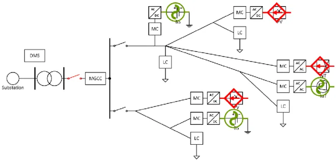
The configuration of the control architecture mainly depends on the existing grid infrastructure. As represented in figure 3, a typical MG hierarchical architecture consists of the distribution management system (DMS), which is responsible for the collaboration between the distribution system operator (DSO), the energy service company (ESCO) and the MG operator; the MG central controller (MGCC), which is responsible for the efficient coordination of the local microsource controllers (MC) and load controllers (LC), provides set points and controls their operation. The MCs are responsible for controlling and monitoring the local distributed generation sources and storage units, while the LCs are responsible for controlling and monitoring the local loads.

Figure 3 – Control architecture of a MG

The hardware includes the main server and remote terminal units (RTU) or intelligent electronic devices (IED) distributed across the grid that receive data from sensors and send control commands to the DER units, loads and circuit breakers [14].

(44)

12

3.2. Droop control method

The droop control is implemented in the controllers of the power converters and allows voltage and frequency control by regulating the shared active and reactive power according to the reference set point [16]. The main idea is to emulate the operation of a typical synchronous generator, reducing frequency as active power increases and decreasing voltage amplitude as reactive power demand increases [20]. The formulation of the droop equations is based on the active and reactive power shared between a bus with voltage V and a power converter with voltage E and angle δ, as represented in figure 4.

Figure 4 – Power flow in a transmission line

The active power P and reactive power Q flowing through a transmission line with impedance Z and angle θ can be described as [21, 22]:

𝑃 =𝑉2 𝑍 ∙ cos 𝜃 − 𝑉∙𝐸 𝑍 ∙ cos(𝜃 + 𝛿) (1) 𝑄 =𝑉2 𝑍 ∙ sin 𝜃 − 𝑉∙𝐸 𝑍 ∙ sin(𝜃 + 𝛿) (2)

(45)

𝑃 = 𝑉 𝑋2_+𝑅2∙ (𝑅 ∙ 𝑉 − 𝐸 ∙ cos 𝛿 + 𝑋 ∙ 𝐸 ∙ sin 𝛿) (3) 𝑄 = 𝑉 𝑋2_+𝑅2∙ (𝑋 ∙ 𝑉 − 𝐸 ∙ cos 𝛿 − 𝑅 ∙ 𝐸 ∙ sin 𝛿) (4)

Given that the inductance in typical transmission lines is X≫R, the resistance, R, can be neglected: 𝑃 =𝑉∙𝐸 𝑋 ∙ sin 𝛿 (5) 𝑄 =𝑉2 𝑋 − 𝑉∙𝐸 𝑋 ∙ cos 𝛿 (6)

If the power angle δ is small, then sinδ=δ and cosδ=1, resulting in the simplified equations: 𝛿 ≅𝑋∙𝑃 𝑉∙𝐸 (7) 𝑉 − 𝐸 ≅𝑋∙𝑄 𝑉 (8)

(46)

14

The previous equations (7) and (8), show that the power angle depends on the active power, while the voltage difference depends on the reactive power. Frequency is related to the power angle, so by regulating the active and reactive power flow, the voltage and frequency parameters can be determined. Finally, the frequency and voltage control through active and reactive power is given by:

𝑓 = 𝑓₀− 𝑘_𝑃 ∙ (𝑃 − 𝑃₀)

(9)

𝑉 = 𝑉₀− 𝑘_𝑄∙ (𝑄 − 𝑄₀)

(10)

Where V0 and f0 are the nominal voltage and nominal frequency respectively, P0 and Q0 are the temporary references for active and reactive power that lead to obtain f0 and V0,

respectively. kP and kQ are the droop control settings for frequency and voltage, respectively. The droop control characteristics plots for frequency and voltage are represented in figure 5.

(47)

As represented in figure 5, an increase of active and reactive power will allow frequency and voltage to decrease following a droop control setting. All the parameters are measured and available locally, allowing frequency and voltage regulation according to the injected active and reactive power without the need for a complex communication structure.

3.3. Hierarchical control

A hierarchical control approach consists in three distinct levels of control, as shown in table III. A first layer of control, the primary control level, is responsible for the inner control of the DER units and maintains the voltage and frequency. A second layer, the secondary control level, compensates the voltage and frequency deviations caused by the first level of control. And a third layer, the tertiary control level, manages the power flow between the MG and the main grid according to economic concerns [23].

Table III – Hierarchical control levels

Implementation Control tasks

Primary Local Voltage and frequency maintenance through P/Q droop control

Secondary Centralized/Decentralized Synchronization & Voltage and frequency deviations correction

Tertiary Decentralized Power flow management & Economically optimal grid operation

3.3.1. Primary control layer

Primary control level provides references to the inner voltage and current control loops of the DER units based on the droop control method and stabilizes the voltage and frequency without a communication between the power converters. The droop control applied to the power converters emulates a synchronous generator, reducing the frequency as active power increases. This principle is implemented in the voltage source converters using the frequency/active power and voltage/reactive power droop control equations.

(48)

MICROGRID ARCHITECTURE EVALUATION FOR SMALL AND MEDIUM SIZE INDUSTRIES 16 𝑓 = 𝑓∗− 𝑘𝑃∙ (𝑃 − 𝑃∗) (11) 𝑉 = 𝑉∗_{− 𝑘} 𝑄∙ (𝑄 − 𝑄∗) (12)

Where f* and V* are the reference values for frequency and voltage, respectively. P* and Q* are the references set points for the active and the reactive absorbed power.

A virtual impedance loop can also be included in the primary control level to adjust the output impedance of the voltage source converters. The output voltage can be expressed proportionally drooped with respect to the output current.

𝑉 = 𝑉∗_{− 𝑍 ∙ 𝐼}

(13)

Where V* is the voltage reference obtained by the conventional droop control equations and Z is the virtual output impedance.

3.3.2. Secondary control layer

Secondary control level ensures that the voltage and frequency deviations are compared with a reference value and regulated towards zero after any variation in power generation and load change. Depending on the MGCC, this control layer can be classified in two main types, centralized and decentralized secondary control. The correction parameters ∆f and ∆V are determined using PI compensators.

∆𝑓 = 𝐾_𝑃𝑓∙ (𝑓∗_{− 𝑓) + 𝐾}

𝐼𝑓∙ ∫(𝑓∗− 𝑓) 𝑑𝑡

(49)

∆𝑉 = 𝐾_𝑃𝑉∙ (𝑉∗− 𝑉) + 𝐾_𝐼𝑉 ∙ ∫(𝑉∗− 𝑉) 𝑑𝑡

(15)

Where KPf and KPV are the proportional gains, and KIf and KIV are the integral gains for frequency and voltage respectively. The droop control equations are modified with the correction parameters for frequency and voltage, ∆f and ∆V.

𝑓 = 𝑓∗− 𝑘𝑃 ∙ (𝑃 − 𝑃∗) + ∆𝑓

(16)

𝑉 = 𝑉∗− 𝑘_𝑄∙ (𝑄 − 𝑄∗) + ∆𝑉

(17)

With a centralized secondary control approach, the control is implemented in the MGCC, which interacts and sends references to all the local controllers. In this approach, the voltage and frequency values are measured and compared with the references sent by the MGCC, the resulting deviation value is then sent to the primary control in order to restore the voltage and frequency. With a decentralized secondary approach, the control is implemented locally on all the local controllers. In this approach the values are measured by each local controller and sent to all the other controllers in order to determine an average deviation to restore the voltage and frequency [24].

3.3.3. Tertiary control layer

Tertiary control level takes into account economic aspects based on real time energy prices and manages the power flow between the MG and the main grid. The power flow is controlled by adjusting the voltage and frequency of the DER units aiming for an economically optimal operation for the MG. The grid active and reactive power values are

(50)

18

measured and compared with the grid reference values P*grid and Q*grid in order to obtain the frequency and voltage references f* and V*.

𝑓∗ _{= 𝐾} 𝑃𝑃∙ (𝑃𝑔𝑟𝑖𝑑∗ − 𝑃𝑔𝑟𝑖𝑑) + 𝐾𝐼𝑃∙ ∫(𝑃𝑔𝑟𝑖𝑑∗ − 𝑃𝑔𝑟𝑖𝑑) 𝑑𝑡 (18) 𝑉∗ _{= K} 𝑃𝑄∙ (𝑄𝑔𝑟𝑖𝑑∗ − 𝑄𝑔𝑟𝑖𝑑) + 𝐾𝐼𝑄∙ ∫(𝑄𝑔𝑟𝑖𝑑∗ − 𝑄𝑔𝑟𝑖𝑑) 𝑑𝑡 (19)

Where KPP and KPQ are the proportional gains, and KIP and KIQ are the integral gains for the active and reactive power respectively.

(51)

4. COMMUNICATION ARCHITECTURE

In order to monitor and control a system with integrated DER, power converters and variant load patterns, an appropriated communication configuration has to be adopted. The selection of the communication architecture for the MG depends on the existing grid design where the control elements are located, the number of DER units, load clusters locations, data rate, maintenance costs and mainly on the communication technology chosen. The communication architecture can be implemented based on a centralized and decentralized approach. With a centralized architecture (one-to-all), the central controller coordinates the intelligent electronic devices (IED) settings for different operating conditions. With a decentralized architecture (all-to-all), a central controller is discarded and each IED uses the information sent from the other IEDs and coordinates the operation settings. The local controllers are simpler in the centralized approach, since they are not in charge of making decisions. The central controller is responsible of making decisions based on data received from the local controllers. In the decentralized approach, each local controller is in charge of processing data and making decisions, requiring more advanced and complex control devices [14].

The data transmission between the power elements and IEDs and between IEDs and the central controller can mainly follow two physical communication technologies, a wired and a wireless communication technology. A wired communication network does not rely on batteries to operate and generally offers higher speeds. The data transmission rate can easily reach up to 1 Gbps or more in optical cable applications, while a wireless network has a data transmission rate of 600 Mbps (in Wi-Fi networks), slightly less reliable and it is more susceptible to interference. On the other hand, a wireless communication network includes lower installation costs, easier installation of remote terminal units (RTU) and flexibility to add new nodes to the existing network [25, 26]. Depending on the technology adopted, the communication system can also integrate both wired and wireless links in parallel to help reducing data traffic congestions in the wired links and improve the availability of the network [27].

(52)

20

4.1. Wireless communication links

There are several wireless communication technologies that are suitable for MG communication networks, such as Wi-Fi, WiMAX, Cellular 3G/4G, ZigBee and Bluetooth [28, 29]. These technologies may follow distinct IEEE standards and can be distinguished by data transmission rate, operating frequency band and range as presented in table IV.

Table IV – Wireless technologies characteristics [29, 30]

Family Data rate Range Frequency

Wi-Fi IEEE 802.11e/s up to 54 Mbps up to 300 m 2.4 GHz / 5 GHz IEEE 802.11n up to 600 Mbps WiMAX IEEE 802.16 75 Mbps up to 100 km 2.5 GHz / 3.5 GHz / 5.8 GHz WPAN ZigBee (IEEE 802.15.4) 20 - 250 kbps up to 75 m 868 MHz / 915 MHz / 2.4 GHz Bluetooth (IEEE 802.15.1) 1 - 3 Mbps 1 - 100 m 2.4 - 2.485 GHz Cellular GSM 14.4 kbps 1 - 10 km 900 - 1800 MHz GPRS 170 kbps 3G 384 kbps – 2 Mbps 1 - 10 km 900 MHz / 2100 MHz (or 850 MHz / 1900 MHz) 3G (HSPA) 14.4 Mbps down 5.75 Mbps up 3G (HSPA+) 84 Mbps down 22 Mbps up up to 5 km 4G (LTE) 326 Mbps down 86 Mbps up up to 5 km 5 - 30 km 30 - 100 km 800 MHz / 1800 MHz / 2600 MHz (or 700 MHz / 1700 MHz / 1900 MHz) 4G (LTE Advanced) 1 Gbps down 500 Mbps up

4.1.1. Wi-Fi

A Wi-Fi network provides a flexible, reliable and high speed local wireless communication based on the IEEE 802.11x standards. Wi-Fi 802.11e and 802.11s standard specifications propose the implementation of the wireless home and local area network (WLAN) on the 2.4 GHz / 5 GHz frequency bands, offering 54 Mbps data transmission speed and range up

(53)

to 300 m. Wi-Fi 802.11n standard specifications propose implementations on the 2.4 GHz / 5 GHz frequency bands up to 300 m with data rates of 600 Mbps. Because Wi-Fi networks operate on the unlicensed spectrum, their deployment is relatively cheap. But at the same time, the use of a crowded unlicensed spectrum also makes Wi-Fi networks more susceptible to interference [29].

4.1.2. WiMAX

A WiMAX network offers a long coverage area and high speed wireless communication based on the IEEE 802.16x standards. WiMAX 802.16 standard specifications define implementation on the 2.5 GHz / 3.5 GHz / 5.8 GHz frequency bands with data transmission speeds of 75 Mbps. It also proposes a coverage area up to a maximum of 100 kms depending on the performance. Other WiMAX IEEE standards allow implementation on higher frequency bands with lower data rates. However, high spectrum frequencies cannot support non-line-of-sight (NLOS) transmission scenarios, requiring a line-of-sight (LOS) scenario to operate, where a path between the receiver and transmitter is visible. WiMAX provides good performance over long distances and supports thousands of simultaneous users. However, a WiMAX network requires a complex network management [29].

4.1.3. ZigBee

A ZigBee network provides a low power and low cost local wireless communication based on the IEEE 802.15.4 standards. It proposes a worldwide use on the 2.4 GHz frequency band (Europe – 868 MHz and North America – 915 MHz) and a typical range up to 75 m with low data rates of 20-250 kbps. The ZigBee Pro supports an increased coverage area up to 1600 m [30]. ZigBee is considered an ideal network for energy metering and management applications that require both low power consumption and low bandwidth with a low deployment cost [31]. This technology offers a simple and cheap solution, making it the most adopted technology for wireless personal area networks (WPAN) in commercial and industrial applications [29].

(54)

22

4.1.4. Bluetooth

A Bluetooth network provides a low power local wireless communication with low deployment costs based on the IEEE 802.15.1 standards. It operates on the 2.4-2.485 GHz frequency band with a data transmission speed of 1-3 Mbps and a coverage area of 1-100 m. Bluetooth networks offers less latency than ZigBee or Wi-Fi networks and can be often used in local monitoring applications [28, 32]. Due to the limited range, both Bluetooth and ZigBee networks are unable to scale to large networks [29]. This technology suffers from security concerns, but it is still widely adopted for wireless personal area networks (WPAN) with low cost deployment.

4.1.5. Cellular 3G/4G

The 3rd Generation (3G) and 4th Generation (4G) cellular networks provide long distance wireless communications with ranges up to 10 km and 100 km, respectively. Cellular 3G operates on the 900 MHz / 2100 MHz frequency band (or 850 MHz / 1900 MHz) with a coverage area of 1-10 km and data rates of 384 kbps to 2 Mbps. 3G (HSPA) offers data download speeds of 14.4 Mbps and data upload speeds of 5.75 Mbps with ranges up to 10 km. 3G (HSPA+) offers an increased data download speed of 84 Mbps and a data upload speed of 22 Mbps with a lower coverage area up to 5 km. Cellular 4G operates on the 800 MHz / 1800 MHz / 2600 MHz frequency band (or 700 MHz / 1700 MHz / 1900 MHz) with an extended range up to 100 km with a performance hit. The optimum and acceptable operation of cellular 4G is at ranges up to 5 km and 5-30 km, respectively. The operation over longer distances up to 100 km has a reduced performance. 4G (LTE) provides a data download speed of 326 Mbps and a data upload speed of 86 Mbps. 4G (LTE Advanced) offers a much higher data download speed of 1 Gbps and data upload speed of 500 Mbps. The low power consumption of terminal equipment and an extensive data coverage area with high flexibility are the main advantages of cellular networks [29]. Furthermore, public cellular networks are already deployed and can be used with no maintenance costs [28]. However, there are high costs associated with the use of a service provider network and there is no guarantee of service during abnormal weather conditions [31].

(55)

4.2. Wired communication links

The MG communication network may also be integrated with physical wired communication links such as PLC, DSL and optical fibre [29, 33]. The wired technologies follow different IEEE and ITU standards and are distinguished by data transmission rate, operating frequency band and range as presented in table V.

Table V – Wired technologies characteristics [29, 30]

Family Data rate Range Frequency

PLC

NB-PLC (ITU-T G.hnem, IEEE

1901.2) up to 500 kbps +150 km 3 - 500 kHz

BB-PLC (ITU-T G.hn, IEEE

1901) up to 10 Mbps up to 1.5 km 1.8 - 250 MHz

Optical fibre

AON (IEEE 802.3ah) 100 Mbps up to 10 km

500 MHz*km PON (BPON (ITU-T G.983),

GPON (ITU-T G.984), EPON (IEEE 802.3ah)) 155 - 2448 Mbps 10 - 60 km xDSL HDSL (ITU G.991.1) 2 Mbps up to 3.6 km 0.1 - 292 kHz ADSL (ITU G.992.1) 8 Mbps down 1.3 Mbps up up to 4 km 25 kHz – 1.1 MHz ADSL2 (ITU G.992.3) 12 Mbps down 3.5 Mbps up up to 7 km ADSL2+ (ITU G.992.5) 24 Mbps down 3.3 Mbps up 25 kHz – 2.2 MHz VDSL (ITU G.993.1) 52 - 85 Mbps down 16 - 85 Mbps up up to 1.2 km 25 kHz – 12 MHz VDSL2 (ITU G.993.1) up to 200 Mbps 300 m – 1.5 km

4.2.1. PLC

Power line communications (PLC) makes use of existing power lines for data communication. A PLC network provides a cost-effective solution with a low maintenance requirement, since a single infrastructure is used for both data and power transmission [29]. The narrowband PLC (NB-PLC) is based on the ITU-T G.hnem and IEEE 1901.2

(56)

24

standards that define a data transmission speed up to 500 kbps on the 3-500 KHz frequency band and a coverage area of 150 km or more. The broadband PLC (BB-PLC) is based on the ITU-T G.hn and IEEE 1901 standards that define a higher data transmission speed up to 10 Mbps on the 1.8-250 MHz with a shorter coverage area up to 1.5 km. BB-PLC is also capable of providing data rates up to 200 Mbps in very short distances by operating on higher frequency bands. Because PLC makes use of a single infrastructure for data and power decreasing the cost of installation, this communication technology is the preferred solution for metering data transmission and the simplest to implement in smart grid applications. However, the noisy and harsh nature of the power line channel affects the data transmission and may decrease the quality of signal [31].

4.2.2. Optical fibre

An optical fibre infrastructure provides long distance communication with high data rates with robustness against radio and electromagnetic interferences. However, optical fibre applications are characterized by high installation costs, high terminal equipment costs and difficulty to upgrade. These disadvantages prevent optical fibre communications from being widely adopted in smart grids [29]. Active optical network (AON) is based on the IEEE 802.3ah standard and offers data transmission speeds of 100 Mbps with a range up to 10 km. AON requires electrically powered switching equipment such as routers or a switch aggregator to manage signal distribution and direct signals to the correct destination. Passive optical network (PON) technologies provide higher data transmission speeds of 155-2448 Mbps with ranges from 10 km to 60 km, depending on the standard used. PON does not require electrically powered switching equipment, instead it uses optical splitters to separate and collect the signals. Optical fibre applications operate on the 500 MHz frequency band for distances of 1 km (500 MHz*km).

4.2.3. DSL

Digital subscriber lines (DSL) uses telephone line infrastructures to transmit digital data. This avoids additional communication infrastructures when a telephone line infrastructure is already deployed [29]. High-bit-rate DSL (HDSL) is based on the ITU G.991.1 and

(57)

supports data transmission rates up to 2 Mbps on the 0.1-292 kHz frequency band and a maximum coverage of 3.6 km. Asymmetric DSL (ADSL) is based on the ITU G.992.1 and provides a data download speed of 8 Mbps and a data upload speed of 1.3 Mbps on the 25 kHz to 1.1 MHz frequency bands with a coverage area up to 4 km. Asymmetric DSL version 2 (ADSL2) is based on the ITU G.992.3 and provides a higher data download speed of 12 Mbps and a higher data upload speed of 3.5 Mbps on the 25 kHz to 1.1 MHz frequency bands with an increased coverage area up to 7 km. Asymmetric DSL version 2 plus (ADSL2+) is based on the ITU G.992.5 and provides increased data download speed of 24 Mbps and a slightly lower data upload speed of 3.3 Mbps on the 25 kHz to 2.2 MHz frequency bands with a coverage area up to 7 km. Very-high-bit-rate DSL (VDSL) is based on the ITU G.993.1 and supports an increased data download speed of 52-85 Mbps and data upload speed of 16-85 Mbps on the 25 kHz to 12 MHz frequency bands with reduced maximum coverage of 1.2 km. Very-high-bit-rate DSL version 2 (VDSL2) supports data transmission speeds up to 200 Mbps with a typical range from 300 m to 1.5 km. In order to use DSL networks, a communication fee must be paid to the telecommunication operator and the network needs to be regularly maintained [29, 31].

4.3. Communication protocols and standards

The Internet protocol suite (TCP/IP) is a set of communication protocols organized into four distinct layers [27]. The application layer is the highest layer and provides protocols that enable process-to-process data communication. Some of the protocols can be Hypertext Transfer Protocol (HTTP), Secure Shell (SSH), Network Timing Protocol (NTP), Distributed Network Protocol (DNP3) and Modbus. The transport layer establishes data channels and provides host-to-host data communication through protocols such as Transmission Control Protocol (TCP) and User Datagram Protocol (UDP). The internet layer provides authentication and defines the addressing and routing structures through internet protocols IPv4 and IPv6. The link layer is the lowest layer and defines methods for the local network communication link. Table VI shows the protocols for each layer of the TCP/IP model.

(58)

26

Table VI – TCP/IP model layers

Layer Protocols Function

1 Application HTTP, SSH, NTP Enables process-to-process data communication

2 Transport TCP, UDP Provides host-to-host data communication

3 Internet IPv4, IPv6 Defines the addressing and routing structures

4 Link Serial, Ethernet Defines methods for communication link

4.3.1. Modbus

Modbus is a communication protocol that enables communication between a server unit and clients connected to the same network. It is often used in supervisory control and data acquisition (SCADA) systems for a robust communication between supervisory units and remote terminal units (RTU). In a MG with Modbus protocol model, the central controller may act as a server while each IED acts as a client. The data communication between the server and clients is made based on polls from the server. Modbus can be transmitted over RS232, RS485 and Ethernet (TCP/IP) using protocol converters.

4.3.2. DNP3

DNP3 is a new communication protocol often used for data acquisition in SCADA systems that provides a reliable and efficient server to client data communication. Unlike the older protocol Modbus, DNP3 allows client units to be updated without waiting for a poll from the server and supports time synchronization with RTUs by including timestamp variants. DNP3 offers a robust communication and compatibility with a wide range of equipment, being widely used in several industrial applications.

(59)

4.3.3. IEC 61850

IEC 61850 is a communication standard that defines data models, events and settings for substation IED configurations. These data models can be mapped to a number of protocols, such as Manufacturing Message Specification (MMS), Generic Object Oriented Substation Event (GOOSE) and Sampled Measured Values (SMV). The IEC 61850 standard enables the integration of protection, control and measurement functions in substation applications.

(60)

(61)

5. MICROGRID ARCHITECTURE

The implementation of low-carbon energy sources into the power grid is an approach that has been made in order to reduce GHG and carbon emissions in the power sector. This environmental effort led to several MG architecture configurations with high penetration of RES [34].

This section presents a basic architecture of a MG and its DG units, storage units and loads. The main purpose of this architecture is to introduce different technologies for the most common energy resources in MGs. The characteristics for these energy resources are summarized in Appendix A. As represented in figure 6, this architecture consists of a HV/MV transformer substation (T1), MV/LV transformers (T2 and T3), groups of distributed generation (G1 and G2) and load clusters (L1 and L2).

(62)

30

5.1. Distributed generation

Distributed generation (DG) units can include photovoltaic (PV) generation, wind turbines (WT), fuel cells (FC) and micro turbines (MT) [35]. The DG units are located within the same grid and aim to fulfil the local demand. Table VII shows characteristics for the most common DG units adopted in MGs.

Table VII – Distributed generation units [36]

Characteristics PV WT FC MT

Availability Location dependent Location dependent Any time Any time

Control Non-controllable Non-controllable Controllable Controllable

Output power DC AC DC AC Conversion Power electronic converter (DC-DC-AC) Power electronic converter (AC-DC-AC) Power electronic converter (DC-DC-AC) Power electronic converter (AC-DC-AC) Power flow control MPPT & DC link voltage control (+P, ±Q)

Turbine speed & DC link voltage control (+P, ±Q)

MPPT & DC link voltage control

(+P, ±Q)

Turbine speed & DC link voltage control (+P, ±Q)

GHG emission None None Low Low

5.1.1. Photovoltaic

A photovoltaic (PV) system converts solar energy into electrical energy by exciting electrons in silicon cells, making this energy source an intermittent RES. The system consists in PV panels that include one or more cell modules and these cells can be wired in parallel to increase current and in series to increase voltage depending on the system requirements.

Major advantages and benefits of a PV system:

 Positive environmental impact;

 Low operation and maintenance costs;

(63)

 Clean and silent operation;

 Generation coincides with peak energy demand.

This solution also brings some disadvantages such as high fixed costs, low cell efficiency, location restrictions and weather dependent. A common way to overcome these disadvantages is to integrate the PV systems with other energy resources.

Solar cells made from crystalline silicon (c-Si) are generally the most common and efficient ones. Depending on the alignment of the silicon molecules and manufacturing process, silicon cells can be made from a single pure crystal of silicon, called monocrystalline (mono-Si) cells and made from an ingot of melted and recrystallized silicon, called polycrystalline (poly-Si) cells. Solar cells can also be made by depositing thin layers of non-crystallized silicon onto a substrate, forming thin-film amorphous (a-Si) cells. Monocrystalline PV panels have the longest service life and also the highest efficiency rates and power output with the least amount of required space. Due to the complicated manufacturing process and purity of the monocrystalline cells, monocrystalline PV panels have the highest production costs and a significant amount of silicon results in waste. Although performance decreases with temperature, monocrystalline technology has a better heat tolerance in warm weather. Polycrystalline PV panels have a slightly lower efficiency and heat tolerance, but the manufacturing process is simpler and costs less, resulting in cheaper panels. Amorphous PV panels are the cheapest to manufacture and can be produced with a flexible substrate, but this technology has the lowest power output and efficiency rates. The typical efficiency rates are around 15% to 23% for monocrystalline PV panels, 13% to 16% for polycrystalline PV panels and 5% to 10% for amorphous PV panels [37]. Table VIII shows the highest confirmed module efficiencies independently measured by a test centre [38].

Table VIII – Solar modules efficiencies [38]

Technology Efficiency (%) Area (cm2) Voc (V) Isc (A) Fill Factor (%)

Crystalline silicon

Monocrystalline silicon 24.4 ± 0.5 13177 (da) 79.5 5.04 80.1

(64)

32

Thin-film

Amorphous silicon 12.3 ± 0.3 14322 (t) 280.1 0.902 69.9

(t) – Total area

(ap) – Aperture area (masked)

(da) – Designated area (masked)

Standard Test Conditions (STC) - Irradiance: 1000 W/m2; Spectrum: AM 1.5; Temperature: 25°C

Table IX shows the comparison between two solar modules, a monocrystalline module and a polycrystalline module as shown in figures 7a) and 7b). Both solar modules are from Trina Solar, which is one of the top ranked solar panel manufacturers. These PV modules are meant for utility applications and they are equal in size and number of cells.

Table IX – Trina Solar modules comparison [39]

Module

DUOMAX M+

Dual glass 72 cell TSM-DEG14 (II)

DUOMAX

Dual glass 72 cell TSM-PEG14

Solar cells Monocrystalline (156.75 x 156.75 mm) Polycrystalline (156.75 x 156.75 mm) Cell orientation 72 cells (6 x 12) 72 cells (6 x 12)

Peak power range

(STC) 335 – 365 Wp 320 – 335 Wp Maximum power voltage (STC) 37.9 – 39.1 V 37.2 – 37.8 V Maximum power current (STC) 8.84 – 9.35 A 8.60 – 8.87 A Module efficiency (STC) 17.1 – 18.6 % 16.3 – 17.1 %