Application of optimization methods to the 2D liquid chromatography

(1)

(2)

(3)

Universidade de Aveiro Departamento de Química

2013

Andreia Santos

Paula

Aplicação de métodos de otimização à cromatografia

líquida 2D

Application of optimization methods to the 2D liquid

chromatography

Dissertação apresentada no Departamento de Química da Universidade de Aveiro para cumprimento dos requisitos necessários à obtenção do grau de Mestre em Química - Especialidade em Química Analítica e Qualidade, realizada sob a orientação científica do Doutor Armando da Costa Duarte, Professor Catedrático do Departamento de Química da Universidade de Aveiro, e da Doutora Regina Maria Brandão de Oliveira Duarte, Investigadora Auxiliar do Centro de Estudos do Ambiente e do Mar (CESAM) da Universidade de Aveiro.

(4)

(5)

(6)

(7)

O Júri

Presidente Prof. Doutor Artur Manuel Soares da Silva

Professor Catedrático do Departamento de Química da Universidade de Aveiro

Prof. Doutora Teresa Alexandra Peixoto da Rocha Santos Professora Associada do ISEIT/Viseu do Instituto Piaget Doutora Regina Maria Brandão de Oliveira Duarte

Investigadora Auxiliar do Centro de Estudos do Ambiente e do Mar (CESAM) da Universidade de Aveiro

(8)

(9)

Agradecimentos Para a realização desta dissertação tive o apoio de diversas pessoas as quais gostaria de deixar o meu Muito Obrigada.

Em primeiro lugar, gostaria de agradecer aos meus orientadores, Doutor Armando da Costa Duarte e Doutora Regina Maria Brandão de Oliveira Duarte pela disponibilidade, compreensão, dedicação e amizade demonstrada durante ano.

Aos meus pais e avó, por todo o apoio, educação e carinho que demonstraram nesta etapa.

Ao meu namorado por me aturar nos bons e maus momentos e por me apoiar sempre.

Aos meus amigos, especialmente à Telma, e colegas de laboratório, especialmente ao João Matos, por toda ajuda e disponibilidade demonstrada durante o desenvolvimento de todo o trabalho. Também agradeço à Sónia e à Catarina todo o apoio. Obrigada pelas gargalhadas e boa disposição.

(10)

(11)

Palavras-chave Cromatografia líquida bidimensional abrangente; otimização; coluna de modo misto de fase reversa/troca aniónica; coluna de fase reversa de octadecil de sílica; amostras de vinho tinto.

Resumo Esta dissertação teve como principal objectivo a aplicação de metodologias quimiométricas de otimização em cromatografia líquida bidimensional abrangente (LC×LC) por forma a determinar as condições ótimas para a separação de amostras de vinho tinto português. Para este estudo, foi utilizada, na primeira dimensão, uma fase estacionária de modo misto de fase reversa/troca aniónica (Acclaim® Mixed-Mode WAX-1, denominação em inglês) e, na segunda dimensão, uma fase reversa de octadecilsílica (C18). O LC×LC foi acoplado a um detector de fotodíodos, a operar na gama de comprimentos de onda de 221 a 400 nm. O modo de eluição por gradiente foi adotado para ambas as dimensões cromatográficas. O planeamento experimental D-Optimal foi considerado o mais adequado para a otimização na primeira dimensão, tendo permitido identificar entre um conjunto de 6 variáveis experimentais (% MeoHi, [Buffer]i, ti, % MeOHf, [Buffer]f, and tf), quais as mais importantes que

afetam a qualidade de separação cromatográfica, em termos unidimensionais, de uma amostra composta de vinhos tintos portugueses. A qualidade de separação cromatográfica foi avaliada utilizando uma função de resposta cromatográfica (CRF, sigla inglesa para “chromatographic response function”)

previamente desenvolvida por Duarte & Duarte (2010) (DCRF), concluindo-se que as variáveis mais importantes são % MeOHi and % MeOHf. A otimização

da separação na segunda dimensão foi efectuada utilizando já o sistema LC×LC, e recorrendo ao método Simplex para o estudo das duas variáveis mais importantes que afectam a eluição por gradiente numa coluna de fase reversa C18: % MeOHi and % MeOHf na fase móvel. A qualidade de separação

cromatográfica bidimensional foi avaliada utilizando uma CRF previamente desenvolvida por Duarte et al. (2010) (DCRFf,2D). Nas condições ótimas

estimadas para a aplicação da técnica de Mixed-Mode WAX-1×C18, para a separação de uma amostra representativa dos vinhos tintos portugueses seleccionados, foram registados 59 picos no espaço cromatográfico, em 150 minutos de tempo total de análise. Utilizando as condições de separação cromatográfica previamente otimizadas, efectuou-se a análise de 4 amostras de vinho tinto português a fim de se verificar a existência, para posterior comparação, de perfis cromatográficos diferentes.

(12)

(13)

Keywords Comprehensive two-dimensional liquid chromatography; optimization; mixed-mode reverse phase/anion exchange column; conventional reverse phase column of octadecyl silica; red wine samples

Abstract The main objective of this work was the application of chemometrics to the optimization of comprehensive two-dimensional liquid chromatography (LC×LC) in order to find the optimal conditions for the separation of samples of Portuguese red wines. A column with a stationary phase mixed-mode reverse phase/anion exchange (Acclaim ® Mixed -Mode WAX -1) was used as the first dimension, and a reverse phase column of octadecylsilica (C18) was used as the second dimension. The LC×LC was coupled to a photodiode detector, operating in the wavelength range of 221-400 nm. A gradient elution mode was adopted for both chromatographic dimensions. The D-Optimal design was considered the most suitable for the optimization of separation in the first dimension (1D) and it allowed from a set of 6 experimental variables (% MeOHi, [Buffer]i, ti,

% MeOHf, [Buffer]f, and tf) the identification of the most relevant for the

quality of chromatographic separation of a composite sample of selected Portuguese red wines. The quality of the chromatographic separation was evaluated using a chromatographic response function (CRF), previously developed by Duarte and Duarte (2010) (DCRF). Thus, it was concluded that the most important variables affecting the separation of the sample in the first dimension are the % MeOHi, and % MeOHf. The optimization of

separation in the second dimension (2D) was performed using now the LC×LC system, and using the Simplex method for the study of two most important variables affecting gradient elution on a reverse phase C18 column: starting and ending of the organic solvent (eg, methanol) concentration in the mobile phase. The quality of the two-dimensional chromatographic separation was evaluated using a CRF previously developed by Duarte et al. (2011) (DCRFf,2D). Under the optimum

conditions for the separation of a composite sample of Portuguese red wines by the technique of Mixed -Mode WAX-1×C18, 59 peaks were recorded in 150 minutes of total analysis time. Using conditions previously optimized a chromatographic separation of 4 Portuguese wine samples was carried out in order to compare chromatographic profiles associated with different samples

(14)

(15)

(16)

(17)

Table of contents

XVII

Table of contents ... XV List of figures ... XIX List of tables ... XXV List of abbreviations ... XXIX

I Aims and structure of dissertation ... 1

1.1. Introduction ... 3

1.2. Aim of the dissertation ... 4

1.3. Structure of the dissertation ... 4

II Two-dimensional liquid chromatography: basic concepts ... 7

2.1. The emergence of comprehensive two-dimensional liquid chromatography (LC×LC) ... 9

2.2. Structure of data in LC×LC ... 10

2.2.1 Removal of background and noise ... 13

2.2.2. Dealing with overlapping ... 16

2.2.2.1. Multivariate curve resolution- alternating least squares (MCR-ALS) ... 17

2.2.2.2. Generalized rank annihilation method (GRAM)... 18

2.2.2.3. Parallel factor analysis – alternating least squares (PARAFAC-ALS) ... 18

2.2.2 Synchronization and shifts of retention time... 20

2.3. Chromatographic responses functions (CRF) ... 21

IIIOptimization in analytical chemistry – basic concepts ... 29

3.1. Introduction ... 31

3.2. Design of experiments ... 31

3.3. Simplex algorithm ... 34

IVApplication of LC×LC applied to the analysis of complex mixtures ... 37

V Experimental conditions for chromatographic analysis of wine samples... 45

5.1. Chemicals ... 47

5.2. Description and preparation of wine samples ... 47

5.3. Instrumentation ... 48

5.4. Chromatographic conditions for experimental design ... 50

5.4.1 Optimization of one-dimensional liquid chromatography (1D-LC) ... 51

5.4.2. Optimization of the second dimension (2D) in LC×LC ... 51

5.5. Software for control and data acquisition ... 53

VISearch of optimum conditions for 1D-LC of wine samples... 55

6.1. Choice of operational details and starting conditions... 57

(18)

Table of contents

XVIII

VII Search of optimum conditions of the 2D in LC×LC of wine samples ... 63

7.1. Choice of operational conditions details and starting conditions ... 65

7.2. Change from D-Optimal design to Simplex ... 69

7.2.1. Choice of operational details and starting conditions ... 69

7.2.2. LC×LC applied to the analysis of wine samples ... 72

7.3. Conclusions ... 76

VIII Final conclusions and further work... 77

References... 81

Annex A: Optimization of 1D-LC ... i

(19)

(20)

(21)

List of figures

XIX

Figure 1: Simulated output at the end of the 2D of a LC×LC system. 11

Figure 2: Assembling the individual chromatograms in the 2D defined by a modulation

time of 2 minutes. 11

Figure 3: Three-dimensional (3D) representation of an interpolated and smoothed

LC×LC chromatogram. 12

Figure 4: Contour plot of a LC×LC chromatogram. 12

Figure 5: Representation of the background signal on a simulated LC×LC

chromatogram. 13

Figure 6: Representation of the noise on a simulated LC×LC chromatogram. 15

Figure 7: Representation of overlapped peaks on a simulated LC×LC chromatogram

and its corresponding one-dimensional chromatogram. 16

Figure 8: Schematic representation of a 1D chromatogram illustrating the parameters for the estimative of resolution between unresolved peaks using equation 2.23

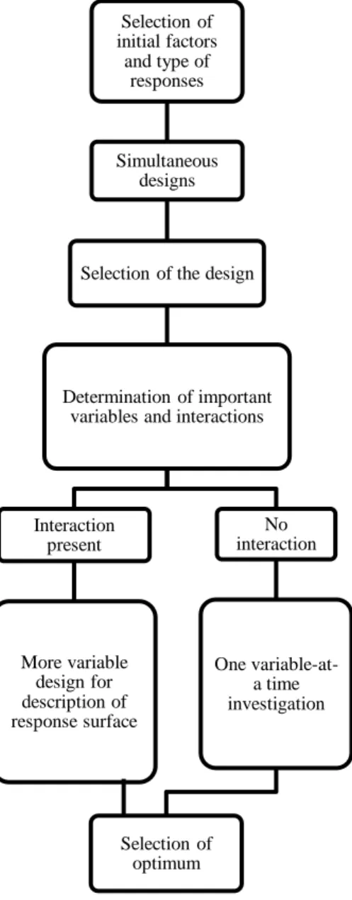
Figure 9: Several steps of an experimental design (Inspired by D.L: Massart, 1997) 32

Figure 10: Example of Simplex optimization. 35

Figure 11: Schematic arrangement of the LC×LC assemblage used in this work (inset: operation positions A and B of the eight-port interfacing valve). 48

Figure 12: Elution program applied into 1D (purple) and 2D (green). 52

Figure 13: Response surface showing the effect of the experimental variables MeOHi

and [Buffer]i on the values of the DCRFf given by the D-optimal design for 1

D. 60

Figure 14: Optimum conditions chromatogram obtained by D-Optimal design. 60

Figure 15: Chromatogram with overlapped peaks obtained by optimization in1D. 61

Figure 16: Response function expressed in terms of DCFR values for the initial and the final % of methanol given by D-Optimal design for the 2D. 66

Figure 17: ANOVA of various models fitted to the results obtained following the

D-Optimal design. 67

Figure 18: ANOVA of the quadratic model suggested as the most appropriate for fitting

the results obtained by the D-Optimal design. 68

Figure 19: Chromatogram obtained by D-Optimal design for 50% of initial methanol

and 5% of final methanol. 69

(22)

List of figures

XX

Figure 21: Two-dimensional liquid chromatography of the composite sample obtained at

optimal conditions. 71

Figure 22: Representation of peaks for optimum condition of composite sample. 72

Figure 23: Representation of the peaks in 2D chromatogram. 72

Figure 24: Chromatogram of red wine sample (EA – Vinho Regional Alentejano (2010))

without any problem of dragging. 73

Figure 25: Chromatogram of red wine sample (EA – Vinho Regional Alentejano (2010))

with dragging. 73

Figure 26: Chromatogram of red wine sample (CICONIA – Vinho Regional Alentejano

(2010)). 74

Figure 27: Chromatogram of red wine sample (Príncipe do Dão (2009)). 74

Figure 28: Chromatogram of red wine sample (Torre de Estremoz – Vinho Regional

Alentejano (2010)). 75

Figure 29: Chromatogram obtained by optimization in the 1D (10% of MeOHi; 40mM

[PPB]I; 2.61 ti; 42.83% of MeOHf; 5mM [PPB]f; 4.93 tf. iii Figure 30: Chromatogram obtained by optimization in the 1D (10% of MeOHi; 50mM

[PPB]I; 3 ti; 40.00% of MeOHf; 10mM [PPB]f; 6 tf. iii Figure 31: Chromatogram obtained by optimization in the 1D (5% of MeOHi; 40mM

[PPB]I; 3 ti; 50.00% of MeOHf; 5mM [PPB]f; 4 tf. iii Figure 32: Chromatogram obtained by optimization in the 1D (10% of MeOHi;

46.43mM [PPB]I; 2 ti; 50.00% of MeOHf; 7.44mM [PPB]f; 4 tf. iv Figure 33: Chromatogram obtained by optimization in the 1D (10% of MeOHi; 50mM

[PPB]I; 3 ti; 40.00% of MeOHf; 10mM [PPB]f; 6 tf. iv Figure 34: Chromatogram obtained by optimization in the 1D (7.46% of MeOHi; 40mM

[PPB]I; 2.46 ti; 40.00% of MeOHf; 10mM [PPB]f; 4 tf. iv Figure 35: Chromatogram obtained by optimization in the 1D (9.39% of MeOHi, 40mM

[PPB]i, 2 ti, 40%MeOHf, 5mM [PPB]f, and 4 tf). v Figure 36: Chromatogram obtained by optimization in the 1D (10% of MeOHi, 50mM

[PPB]i, 3 ti, 50%MeOHf, 5mM [PPB]f, and 4 tf). v Figure 37: Chromatogram obtained by optimization in the 1D (7.75% of MeOHi,

45.93mM [PPB]i, 2.48 ti, 50%MeOHf, 10mM [PPB]f, and 5.03 tf). v Figure 38: Chromatogram obtained by optimization in the 1D (5% of MeOHi, 50mM

(23)

List of figures

XXI

Figure 39: Chromatogram obtained by optimization in the 1D (10% of MeOHi, 50mM

[PPB]i, 3 ti, 50%MeOHf, 5mM [PPB]f, and 4 tf). vi Figure 40: Chromatogram obtained by optimization in the 1D (10% of MeOHi, 40mM

[PPB]i, 2.55 ti, 40%MeOHf, 7.88mM [PPB]f, and 6 tf). vi Figure 41: Chromatogram obtained by optimization in the 1D (5% of MeOHi, 50mM

[PPB]i, 2 ti, 50%MeOHf, 5mM [PPB]f, and 4 tf). vii Figure 42: Chromatogram obtained by optimization in the 1D (10% of MeOHi, 50mM

[PPB]i, 2.36 ti, 44.49%MeOHf, 10mM [PPB]f, and 4 tf). vii Figure 43: Chromatogram obtained by optimization in the 1D (10% of MeOHi, 40mM

[PPB]i, 2 ti, 50%MeOHf, 5mM [PPB]f, and 6 tf). vii Figure 44: Chromatogram obtained by optimization in the 1D (10% of MeOHi, 50 mM

[PPB]i, 2.36 ti, 44.49%MeOHf, 10mM [PPB]f, and 4 tf). viii Figure 45: Chromatogram obtained by optimization in the 1D (5% of MeOHi, 50 mM

[PPB]i, 2 ti, 40%MeOHf, 8.34mM [PPB]f, and 6 tf). viii Figure 46: Chromatogram obtained by optimization in the 1D (5% of MeOHi, 40 mM

[PPB]i, 3 ti, 50%MeOHf, 10mM [PPB]f, and 6 tf). viii Figure 47: Chromatogram obtained by optimization in the 2D (5% of MeOHi, 40mM

[PPB]i, 3 ti, 40%MeOHf, 10mM [PPB]f, and 4 tf). ix Figure 48: Chromatogram obtained by optimization in the 1D (5% of MeOHi, 40mM

[PPB]i, 2 ti, 50%MeOHf, 10mM [PPB]f, and 4 tf) ix Figure 50: Chromatogram obtained by optimization in the 1D (5% of MeOHi, 43.21mM

[PPB]i, 2 ti, 40%MeOHf, 5mM [PPB]f, and 6 tf). ix Figure 51: Chromatogram obtained by optimization in the 1D (9.69% of MeOHi, 50 mM

[PPB]i, 2.08 ti, 41.23%MeOHf, 5.41mM [PPB]f, and 4 tf). x Figure 52: Chromatogram obtained by optimization in the 1D (5% of MeOHi, 40 mM

[PPB]i, 2 ti, 50%MeOHf, 10mM [PPB]f, and 4 tf). x Figure 53: Chromatogram obtained by optimization in the 1D (8.09% of MeOHi, 40 mM

[PPB]i, 3 ti, 50%MeOHf, 7.05mM [PPB]f, and 5.66 tf). x Figure 54: Chromatogram obtained by optimization in the 1D (10% of MeOHi,

45.49mM [PPB]i, 3 ti, 47.%MeOHf, 5mM [PPB]f, and 6 tf). xi Figure 55: Chromatogram obtained by optimization in the 1D (10% of MeOHi, 50mM

[PPB]i, 2 ti, 50%MeOHf, 10mM [PPB]f, and 6 tf). xi Figure 56: Chromatogram obtained by optimization in the 2D (5.70% of MeOHi, 40mM

(24)

List of figures

XXII

Figure 57: Chromatogram obtained by optimization in the 1D (5% of MeOHi, 50 mM

[PPB]i, 3 ti, 40%MeOHf, 5mM [PPB]f, and 4.97 tf). xii Figure 58: Chromatogram obtained by optimization in the 1D (10% of MeOHi, 50 mM

[PPB]i, 2 ti, 50%MeOHf, 10mM [PPB]f, and 6 tf). xii Figure 59: Chromatogram obtained by optimization in the 1D (5% of MeOHi, 40 mM

[PPB]i, 2 ti, 50%MeOHf, 5mM [PPB]f, and 6 tf). xii Figure 60: Chromatogram obtained by optimization in the 1D (5% of MeOHi, 50mM

[PPB]i, 2.44 ti, 40%MeOHf, 5mM [PPB]f, and 4 tf). xiii Figure 61: Chromatogram obtained by optimization in the 1D(6.63% of MeOHi, 40mM

[PPB]i, 2 ti, 49.22%MeOHf, 5mM [PPB]f, and 4 tf). xiii Figure 62: Chromatogram obtained by optimization in the 1D (5% of MeOHi, 50mM

[PPB]i, 3 ti, 50%MeOHf, 10mM [PPB]f, and 4 tf). xiii Figure 63: Chromatogram obtained by optimization in the 1D (10% of MeOHi, 43.29

mM [PPB]i, 2 ti, 40%MeOHf, 10mM [PPB]f, and 4.97 tf). xiv Figure 64: Chromatogram obtained by optimization in the 1D(6.63% of MeOHi, 40 mM

[PPB]i, 3 ti, 40%MeOHf, 5mM [PPB]f, and 6 tf). xiv Figure 65: Chromatogram obtained by optimization in the 1D (10% of MeOHi, 40mM

[PPB]i, 3 ti, 50%MeOHf, 10mM [PPB]f, and 4 tf). xiv Figure 66: Chromatogram obtained by optimization in the 1D (5% of MeOHi, 50mM

[PPB]i, 3 ti, 48.91%MeOHf, 5mM [PPB]f, and 4 tf). xv Figure 67: Chromatogram obtained by optimization in the 1D (5% of MeOHi, 50mM

[PPB]i, 2.76 ti, 40%MeOHf, 10mM [PPB]f, and 6 tf). xv Figure 68: Chromatogram obtained by optimization in the 1D (5% of MeOHi, 40 mM

[PPB]i, 2 ti, 40%MeOHf, 6.91mM [PPB]f, and 4.42 tf). xv Figure 69: Chromatogram obtained by optimization in the 1D (10% of MeOHi, 44.29

mM [PPB]i, 3 ti, 40%MeOHf, 5mM [PPB]f, and 4 tf). xvi Figure 70: Chromatogram obtained by optimization in the 1D (8.72% of MeOHi, 40mM

[PPB]i, 2 ti, 44.72%MeOHf, 10mM [PPB]f, and 6 tf). xvi Figure 71: Chromatogram obtained by optimization in the 1D (5% of MeOHi, 50mM

[PPB]i, 3 ti, 50%MeOHf, 5mM [PPB]f, and 6 tf). xvi Figure 72: Chromatogram obtained by optimization in the 1D (5.39% of MeOHi,

40.31mM [PPB]i, 2.91 ti, 40%MeOHf, 5mM [PPB]f, and 4.03 tf). xvii Figure 73: Chromatogram obtained by optimization in the 1D (5% of MeOHi, 50mM

(25)

List of figures

XXIII

Figure 74: Chromatogram obtained by optimization in the 1D (10% of MeOHi, 50mM

[PPB]i, 2 ti, 40%MeOHf, 5mM [PPB]f, and 6 tf). xvii Figure 75: Chromatogram obtained by optimization in the 2D (25% of MeOHi, and

25%MeOHf). xxi

Figure 76: Chromatogram obtained by optimization in the 2D (35% of MeOHi, and

28%MeOHf). xxi

35%MeOHf). xxi

32%MeOHf). xxii

34%MeOHf). xxii

42%MeOHf). xxii

39%MeOHf). xxiii

Figure 82: Chromatogram obtained by optimization in the 2D(15% of MeOHi, and

38%MeOHf). xxiii

28%MeOHf) xxiii

39%MeOHf). xxiv

33%MeOHf). xxiv

37%MeOHf). xxiv

44%MeOHf). xxv

(26)

(27)

(28)

(29)

List of tables

XXVII

Table 1: Different weights for the parameters of DCRFf equation, used for different

analytical scenarios. 25

Table 2: Survey of the studies published after 2008, inclusive, using LC×LC for the

analysis of complex samples. 40

Table 3: Experimental variables and their ranges of variation used in the optimization

procedure for the 1D. 50

Table 4: Experimental design table produced by D-Optimal design for the 1D, using

the Design-Expert software version 7.00. 58

Table 5: Optimum values of each experimental variable achieved by D-optimal design

for 1D. 59

Table 6: Experimental design generated by Design-Expert software version 7.0.0, for

the 2D. 66

(30)

(31)

List of abbreviations

(32)

(33)

List of abbreviations

XXXI ALS Alternating Least Squares

ANOVA Analysis of Variance

AU Arbitrary Units

BSA Bovine Serum Albumin

COWA Correlation Optimized Warping Algorithm CAD Aerosol-Charged Detector

CRF Chromatographic Response Function D-PS Deuterated Polystyrene

DAD Diode Array Detector

DCRF Duarte’s Chromatographic Response Function

DMF N,N-dimethylformamide

ELSD Evaporative Light Scattering Detector ESI Electrospray Ionization

FTIR Fourier Transform Infrared Spectroscopy

GC×GC Comprehensive Two-Dimensional Gas Chromatography GRAM Generalized Rank Annihilation Method

H-PS Protonated Polystyrene

HILIC Hydrophilic Interaction Liquid Chromatography HPLC High Performance Liquid Chromatography HPMC Hydroxypropylmethylcellulose

IR Infrared

LC×LC Comprehensive Two-Dimensional Liquid Chromatography LCLC Liquid Chromatography at Critical Conditions

LS Light Sensor

MCR Multi Curve Resolution

MS Mass Spectrometry

NBA 3-Nitrobenzyl Alcohol

NOM Natural Organic Matter

NP Normal Phase

PALC Per Aqueous Liquid Chromatography PARAFAC Parallel Factor Analysis

(34)

List of abbreviations

XXXII

PEO Polyethylene Oxide

PL-FA Pony-Lake Fulvic Acids

PS Polystyrene

RI Refractive Index

RP Reversed Phase

SEC Size Exclusion Chromatography

SCX Strong Cation Exchange

SR-FA Suwannee River Fulvic Acids S/N Signal-to-noise ratio

TCB Trichlorobenzene

THF Tetrahydrofuran

TOF Time of Flight

UV Ultra-Violet

WCX Weak Cation Exchange

1D-LC One-Dimensional Liquid Chromatography 2D-LC Two-Dimensional Liquid Chromatophy

1D One-Dimensional 2D Two-Dimensional 3D Three-Dimensional 1 D First Dimension 2 D Second Dimension

λExc Excitation Wavelength

(35)

I

(36)

(37)

(38)

(39)

Aims and structure of dissertation

3

1.1. Introduction

Lately, and due to the fast progress of science in many fields, there has been a growing interest in multidimensional techniques that allow analysing complex matrices. From the many available techniques, the one chosen for this work was two–dimensional liquid chromatography (2D-LC), mostly because of its increased peak capacity, selectivity, and resolution (as compared to one-dimensional liquid chromatography (1D-LC)), and also because it is a chromatographic technique still under development.

The main goal of this thesis was to develop optimization strategies with the aid of chemometric tools for deducing the best experimental conditions, both in the first and second dimensions, for the subsequent analysis of red wine samples by comprehensive two-dimensional liquid chromatography (LC×LC) in order to compare their chromatographic profiles. Such studies are very scarcely found in literature. Ideally, it would be useful to optimize both dimensions simultaneously, but in practice such procedure is not attainable, mostly because the separation conditions in the second dimension (2D) depends on the experimental conditions of the first dimension (1D), and varying both conditions simultaneously would threaten any conclusion on the best separation conditions in both dimensions.

For this work, red wine samples were chosen as the matrix for analysis since this beverage is well appreciated in the Mediterranean, and contains large amounts of antioxidants, which have beneficial effects on health. The majority of antioxidants present in red wine play an important role against oxidative damage, which is responsible for the process of aging and for many degenerative conditions like Alzheimer's, Parkinson’s, and Huntington’s (Gazova et al., 2013), but also type 2 diabetes (Napoli et al., 2005) and cancer (Kraft et al., 2009). Phenolic compounds (polyphenols and flavonoids), which have antioxidant and anti-inflammatory activity, make up a large family of naturally occurring compounds in red wine (Verma and Pratap, 2010) and a very important polyphenol is the resveratrol (Das et al., 2011), which prevents heart diseases.

(40)

Chapter I

4

1.2. Aim of the dissertation

As previously mentioned, this dissertation has as its main goal the optimization of the separation conditions in LC×LC for the untargeted separation of compounds contained in red wine samples. For performing this optimization process, it was prepared a composite sample containing 1 mL of each wine sample. Both chromatographic dimensions were optimized independently and with the same columns that were subsequently used in LC×LC. The separation system comprised, in the first dimension (1D), a mixed-mode reversed-phase/anionic exchange column (Acclaim® Mixed-Mode WAX-1), and in the second dimension (2D), a classic C18 reversed phase (RP) column (Kromasil® RP-C18). The effluent of the 2D column was monitored using a diode array detector (DAD). The separation conditions were firstly optimized for the 1D, using the one-dimensional liquid chromatography (1D-LC) approach. Afterwards, the chromatographic conditions for the 2D were optimized using the LC×LC approach. In this optimization process, two algorithms were applied for evaluating the quality of the separation of the red wine samples: the quality of separation in the 1D was assessed using the chromatographic response function (CRF) developed by Duarte and Duarte (2010) for a 1D-LC approach, whereas the quality of separation in the 2D was assessed using the chromatographic response function (DCRFf,2D) developed by Duarte et al. (2011) for a LC×LC approach.

1.3. Structure of the dissertation

This dissertation is divided into eight chapters. Chapter I describe the aims and the structure of this dissertation, providing an overview of the work as well as its organization. Chapter II contains a brief introduction on the basic concepts of 2D-LC, as well as the structure and the processing of the data sets obtained with such technique. Lastly, some issues that may occur when using this technique are discussed together with the

(41)

Aims and structure of dissertation

5

chromatographic response functions that were used to evaluate the quality of separation in the chromatograms.

Chapter III includes details about the optimization process as a whole, as well as a brief discussion on the chemometric methods (D-Optimal and Simplex) used in this work for the optimization of the conditions in both 1D and 2D.

Chapter IV describes the application of LC×LC to the analysis of complex samples, and it includes a literature review on the studies where this technique has been applied.

Chapter V contains all the chromatographic conditions, some of the preliminary results regarding the optimization processes, as well as a description of the instrumentation applied in this work.

Chapter VI introduces and discusses the results obtained from the optimization process applied to the 1D chromatography to the wine samples.

Chapter VII contains the results, discussion, and main conclusions of the optimization process of the 2D of the LC×LC system.

Chapter VIII contains the final conclusions and suggestions for further work. Finally, there is a list of references, followed by Annexes A and B containing additional experimental data obtained in this work.

(42)

(43)

II

Two-dimensional liquid

chromatography: basic concepts

(44)

(45)

The two-dimensional liquid chromatography: basic concepts

9

2.1. The emergence of comprehensive two-dimensional

liquid chromatography (LC×LC)

Nowadays, there has been a growing interest in multidimensional techniques since they have far great resolving power and allows analysing complex matrices when compared with 1D chromatography. One of multidimensional chromatographic techniques that are in an exponential growth, and consequently the subject of a large number of publications, is the 2D-LC. Liquid chromatography techniques are characterized by a variety of separation mechanisms with different selectivity, and the separation in 2D-LC is performed by means of two dimensions, having different or similar separation mechanisms. According to the review of François et al. (2009), the major advantage of using two dimensions is the high peak capacity that can be obtained, which means the reduction of overlapping peaks. The same authors reported that there are two possible schemes of operation in 2D-LC: a) off-line, where all fractions are collected and stored for an indefinitely period of time and, afterwards, the solvent is evaporated, and then each fraction is re-dissolved and re-injected into a second column (i.e., the 2D); and b) on-line, where the sample are transferred from the 1D to the 2D. According to the work of Fairchild

et al. (2009), the best peak capacity is obtained with the off-line scheme, but at expenses of

a long time of analysis. In on-line 2D-LC systems, there are two modes of operation (van Mispelaar et al., 2003, Gray et al., 2004, Matos et al., 2012): a) heart-cutting, where in only the peaks of interest which are separated in the 1D, are further separated in the 2D; and b) comprehensive (usually abbreviated as LC×LC (Marriott et al., 2012)), where the effluent from the first column is constantly sampled and re-injected into the second column, by an interfacing valve. An advantage of the heart-cutting operation mode is that only the components of interest will be analysed through both dimensions, whereas in the comprehensive mode, the whole sample is analysed throughout both dimensions, allowing, therefore, a better separation of the sample components. Donato et al. (2011) also referred that the on-line method is the most convenient, because losses can be minimized when working with very small amounts of sample.

(46)

Chapter II

10

As referred in the review work of Tranchida et al. (2004), the concept of comprehensive chromatography emerged with thin-layer chromatography in 1944, and according to the reviews of Stoll et al. (2007) and Matos et al. (2012), LC×LC was the first type of multidimensional chromatographic technique, which was developed by Erni and Frei in 1978. This work was followed by that of Bushey and Jorgenson (1990), and was just only a decade later that the comprehensive 2D gas chromatography (GC×GC) took the first steps. Phillips and Beens (1999) highlighted in their work that was only after the development of GC×GC that the multidimensional chromatography has become more relevant as a separation science, and the GC×GC analysis attracted more attention than the LC×LC technique.

A literature survey also shows that the application of the LC×LC technique has been mostly focused in the analysis of foodstuffs and beverages (Kivilompolo et al., 2008, Dugo et al., 2009, Montero et al., 2013, Larson et al., 2013, Bailey and Rutan, 2013), macromolecules (such as polymers and copolymers) (Greiderer et al., 2011, Lee et al., 2011, Sinha et al., 2012, Malik et al., 2012), biological tissues (Jeong et al., 2010, Scoparo

et al., 2012, Cai et al., 2012, Halquist et al., 2012), and natural organic matter (NOM)

(Duarte et al., 2012).

2.2. Structure of data in LC×LC

A LC×LC system produces a huge amount of information, which can be in the order of millions of data points, in a short period of time (Stoll et al., 2007, François et al., 2009). When the LC×LC is coupled with a spectrophotometer detector (e.g., a DAD) or a mass spectrometry (MS) detector, the acquired chromatograms comprise an enormous number of data points and, thus, the real-time acquisition of data produces huge files. These data sets need specific processing software for a quick and adequate chemical identification, and classification of complex peaks and, consequently, extract the maximum amount of information. For better understanding the structure of LC×LC data, it is

(47)

11

important to start at looking at an example of a simulated chromatogram, as shown in Figure 1, obtained from a hypothetical detector positioned at the end of the 2D.

Figure 1: Simulated output at the end of the 2D of a LC×LC system.

In Figure 1, each modulation period of 2 minutes contains the chromatographic profile of each fraction of the sample exiting from the 1D column. Each fraction is collected during 2 minutes in one of the 2 identical loops of an interfacing valve, being then transferred to the 2D column where it is separated. The data shown in Figure 1 contains information that has to be assembled in order to show the individual 1D chromatograms that are stacked in each modulation period of 2 minutes. For example, the chromatogram in violet color in Figure 1, from minute 18 to minute 20, is placed in Figure 2 in time 18 (also in violet). Figure 2 shows the whole dataset of Figure 1, but now plotted in the two chromatographic dimensions of an LC×LC system

Figure 2: Assembling the individual chromatograms in the 2D defined by a modulation time of 2

minutes. 0 2 4 6 8 10 12 14 16 18 20 22 24 26 28 30 32 34 36 38 40 42 44 46 48 50 52 54 56 58 60 0 0.1 0.2 0.3 0.4 0.5 0.6 0.7 0.8 0.9 1

Time of analysis [min]

In te nsi ty [A U ] 0 10 20 30 40 50 60 0 0.5 1 1.5 2 0 0.2 0.4 0.6 0.8 1 2nd_{Dimension [min]} 1st_{Dimension [min]} In te n si ty [A U ]

(48)

Chapter II

12

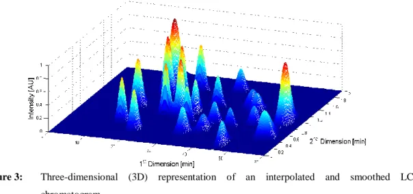
The interpolation and smoothing of the data assembled in Figure 2, for a given grid size (2 min×0.01 min, in this case) allow obtaining a three dimensional (3D) representation of the 2D chromatographic data, as shown in Figure 3, where a color code must be used for highlighting the values of intensity of the analytical signal.

Figure 3: Three-dimensional (3D) representation of an interpolated and smoothed LC×LC

chromatogram.

An alternative to the 3D representation of a 2D chromatogram is shown in Figure 4, under the form of a contour plot, which can be considered an excellent tool for the visualization of 3D representations. The use of a color code associated with the peak intensity allows an easy assessment of the distribution and resolution of the chromatographic peaks.

Figure 4: Contour plot of a LC×LC chromatogram.

1st_{Dimension [min]} 2 nd D im en si on [m in ] 0 10 20 30 40 50 60 0 0.5 1 1.5 2

(49)

13

In ideal 2D chromatography, the above mentioned representations may not be as clear as one would like. There are artifacts, such as background fluctuations and noise (Reichenbach et al., 2003, Zhang et al., 2007, Zeng et al., 2011, Amigo et al., 2010, Matos

et al., 2012, Paraster and Tauler, 2013), overlapped peaks (Stoll et al., 2007, Amigo et al.,

2010, Allan and Rutan, 2011), and shifts in retention time (Fraga et al., 2001, van Mispelaar et al., 2003, Johnson et al., 2004, Pierce et al., 2005, Zhang et al., 2008, Alen and Rutan, 2011, Matos et al., 2012, Yu et al., 2013, Bailey and Rutan, 2013) that should be removed or avoided in order to glean chemical information from the 2D chromatograms. These types of artifacts are common to other 2D separation methods (e.g. GC×GC) and the way to remove them is the same as in any of these systems.

2.2.1 Removal of background and noise

The raw data provided by 2D chromatograms are not always ready for their immediate interpretation because it may contain artifacts, such as background and noise that hinder the extraction of chemical information. Background can be understood as any kind of signal not related to the analyte that causes a systematic interference, as shown in Figure 5, and according to Pierce et al. (2012) its removal is the first step most usually performed in chromatographic data analysis.

Figure 5: Representation of the background signal on a simulated LC×LC chromatogram.

0 ₁₀ 20 ₃₀ 40 50 ₆₀ 0 0.5 1 1.5 2 0 0.2 0.4 0.6 0.8 1 2st_{Dimension [min]} 1st_{Dimension [min]} In te n si ty [A U ]

(50)

Chapter II

14

Reichenbach et al. (2003) suggested an algorithm based on image processing software for background estimation and removal, taking into consideration the statistical and structural properties of different regions of pixels observed on the images obtained in their work with GC×GC. Amigo et al. (2010) proposed another two methods to solve the problem of background removal: a) fit a certain curve (e.g. polynomial) to be able to subtract this curve from the overall signal; and b) model the baseline as part of an overall factor model. The first method is the most easily to be used but it does not provide always the best data quality, while the second approach is an added benefit of the factor model and cannot be taken as a separate component. Zhang et al. (2007) also developed a chemometric method to be used in trilinear data from 2D separation instruments coupled to multichannel detectors. The main idea of this method is to model the background variations on the raw datasets by subtracting the individual signal of background drift from the original raw chromatographic data, thus removing the three dimensional drift. This technique can be applied for all 2D separations coupled to multichannel detectors. Another methodology was developed by Zeng et al. (2011) for dealing with the background consisting in the application to each 2D chromatographic peak, a baseline correction as well as a “moving windows average” method for data smoothing.

As pointed out by Matos et al. (2012), one strategy to elude the background problem is to avoid changes in the composition of the mobile phase, as well as reduce to a minimum the variations in columns temperature, pressure, and fluctuations caused by the interfacing valve.

Noise is another interference generally observed in analytical signals (Matos et al., 2012), which is usually related to the sensitivity of the detector. An example of simulated chromatogram with noise interference is given in Figure 6. The noise refers to any random variation occurring in the signal. These non-systematic variations can cause quantification problems associated with changes in both the shape and the elution time of the peaks (Matos et al., 2012). This interference may be reduced by applying smoothing algorithms, but it is particularly difficult in practice to separate the noise of the signal from the background, particularly when the signal-to-noise ratio (S/N) is low (Parastar and Tauler, 2013).

(51)

15

Figure 6: Representation of the noise on a simulated LC×LC chromatogram.

Most of time, it is not easy to separate background from noise and some authors use the same method to separate these two artifacts. Therefore, a completely different and alternative method based on the application of algorithms of image processing has been suggested by Reichenbach et al. (2003) for dealing with the background and noise in 2D chromatography. The authors claim that this method takes advantage of the following specific structural and statistical properties of the background from the images of 2D chromatograms, namely: a) dead-bands, which are the regions without analytical signal; b) the constant value of the average of background level, which does not change much in comparison with the characteristic peak widths; and c) the random nature of noise has the same statistical properties of the random noise.

On the other hand, according to Zhang et al. (2007), there are two methods to overcome the interferences caused by the background and noise: the first is to use the “mean centering”, and for its implementation the background must be stable; the second is to remove the background by subtraction of a blank chromatographic run. However, the subtraction of the response of the eluent does not always provide acceptable results due to two main sorts of variations: a) the variations in the response intensity of the spectrum of the eluent during a chromatographic run; and b) the occurrence of small shape changes in the spectrum of the eluent.

0 10 20 30 40 50 60 0 0.5 1 1.5 2 0 0.2 0.4 0.6 0.8 1 2nd dimension [min] 1st dimension [min] In te n si ty [A U ]

(52)

Chapter II

16

2.2.2. Dealing with overlapping

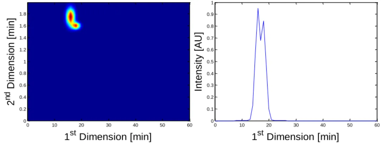
In their work, Stoll et al. (2007) refer that another problem usually detected is the occurrence of overlapped peaks, thus becoming difficult, if not impossible, to quantify the individual peaks. Figure 7 shows a simulated occurrence of overlapped peaks in the LC×LC data structure and its corresponding 1D chromatogram.

Figure 7: Representation of overlapped peaks on a simulated LC×LC chromatogram and its

corresponding one-dimensional chromatogram.

As noted by Allen and Rutan (2012), two methods can be applied for the quantification of overlapped peaks: integration and multi-way analysis. The integration method consists on the summation of the areas of consecutive 2D peaks that contain a single 2D peak. This method has already been discussed by van Mispelaar et al. (2003) and they referred that it is only applied when there is a complete separation at the baseline level between adjacent 2D peaks. So, Bailey and Rutan (2011) developed an integration method to address the concern of van Mispelaar et al. (2003) when working with LC×LC systems. The multi-way algorithms proposed for resolving overlapped peaks encompass the multivariate curve resolution-alternating least squares (MCR-ALS), the generalized rank annihilation method (GRAM), and the parallel factor analysis- alternating least squares (PARAFAC-ALS). 1st Dimension [min] 2 n d D im ens ion [m in] 0 10 20 30 40 50 60 0 0.2 0.4 0.6 0.8 1 1.2 1.4 1.6 1.8 0 10 20 30 40 50 60 0 0.1 0.2 0.3 0.4 0.5 0.6 0.7 0.8 0.9 1 1st Dimension [min] Int ens it y [ AU ]

(53)

17

2.2.2.1. Multivariate curve resolution- alternating least squares

(MCR-ALS)

Hantao et al. (2012) reported that “the main goal of any MCR method is to transform the raw experimental data into a simple composition-weighted linear additive model of pure responses, with a single term per component contribution”. This method is widely used to resolve the issues caused by overlapping peaks in the analytical response, and it is especially used in 2D separations. As a non-iterative method, MCR searches for a single solution in which the pure variables are uniquely deﬁned according to the mathematical principles involved, and the final objective is to analyze each individual constituent in its pure chromatograms (Stoll et al., 2007). One widely used technique encompasses the connection of the MCR method with the ALS algorithm (MCR-ALS), which consists of a multivariate curve fitting technique that also allows to separate dataset components by least squares optimization of chemical data structure using mathematical constraints, such as non-negativity, unimodality, and multilinearity (Bailey and Rutan, 2011). The advantage of using the MCR-ALS method can be seen in the work of Jalali-Heravi et al. (2011), who applied GC-MS for the analysis of rosemary oil, resulting in the detection of 68 compounds. With the application of MCR-ALS, the number of compounds that were able to be identified increased to 99. Bailey and Rutan (2011) applied LC×LC-DAD for the analysis of human urine samples and for quantification purposes. The authors used MCR-ALS with only two constraints (non-negativity and selectivity) and did not apply the multilinearity constraint because the degree of retention time shifting from sample to sample, which occurs in both 1D and 2D chromatograms, is significant enough to prevent the validity of either the trilinearity or quadrilinearity assumptions. According to the same authors, the major disadvantage of this method is the lack of complete automation since it requires intervention of the analyst, but this intervention can be easily handled and it becomes very fast from the point of view of implementation. As reviewed by Arancibia

et al. (2012), a significant advantage of the MCR-ALS is that this algorithm does not

(54)

Chapter II

18

2.2.2.2. Generalized rank annihilation method (GRAM)

The GRAM is a non-iterative algorithm used for qualitative and quantitative analysis (Ferré and Comas, 2011) and it is particularly useful in chromatography, for the quantification of analytes that usually co-elute with interferences existing in complex samples. This method requires a previous calibration step for comparison with the obtained chromatograms and they should be perfectly matched. The start-up of the GRAM requires an input of an estimate of the number of different components existing in the samples under study (Fraga and Corley, 2005). The key requirement for GRAM application is that the two data matrices corresponding to the sample and the standard must be trilinear, thus becoming necessary to ensure that the peaks associated with the components of interest have the same retention time and the same profile in both the sample and the standard chromatograms (Matos et al., 2012). Although GRAM is a non-iterative method, this technique tends to be computationally faster, but it has the limitation of dealing with up to three-way data sets, since only two samples can be analysed at a time, while other algorithms, such as PARAFAC-ALS, can deal with datasets of higher dimensions (Stoll et

al., 2007). The GRAM has been successfully applied in various studies using data obtained

by GC×GC, such as in the analysis of fuels (Bruckner et al., 1998, Prazen et al., 1999), ethylbenzene and m-xylene in modified white gasoline (Bruckner et al., 1998), methyl tert-butyl ether (Prazen et al., 1999), and aromatic isomers (Fraga et al., 2000).

2.2.2.3. Parallel factor analysis – alternating least squares

(PARAFAC-ALS)

The PARAFAC is one of the most widely applied multi-way method, especially for resolving overlapping peaks occurring in 2D chromatograms (Fraga and Corley, 2005, Amigo et al., 2010, Allen and Rutan, 2012), identifying spectral signals (Sinha et al., 2004), removing background signals, and improving S/N (Porter et al., 2006, Parastar and Tauler, 2013). Additionally, the PARAFAC is a mathematical model well suited to deal with 4-way data sets (Allen and Rutan, 2011).

(55)

19

The main requirements for the use of the PARAFAC model is that the component solutions produced must be unique and true if the correct number of components is selected and, thus, the data must obey the multilinearity rule (Allen and Rutan, 2011). It is of paramount importance to select the correct number of components, because if the components are not well selected then the obtained results may not be correct. The first algorithm used to adjust the parameters of the PARAFAC model was the ALS, since it is able to handle unresolved chemical components in three-way or even higher-order data array (Bro, 1997). The estimation of the number of appropriate factors in the PARAFAC model is a very difficult task. Typically, this value is estimated by the sum of interferences and analytes present in the 2D chromatogram, but it is extremely hard to know in advance that number, especially in the presence of a low S/N and overlapping peaks. In order to overcome this problem, Hoggard and Synovec (2007) proposed an algorithm that it is able to select automatically the number of factors to be used by PARAFAC. The models of PARAFAC are automatically generated having an incrementally higher number of factors until mass spectral matching of the corresponding loadings in the model against a target analyte mass spectrum indicates that over fitting has occurred. Then, the model selected simply has one less factor than the over fitted model. So, this model selection approach is viable across the detection range of the instrument from overloaded analyte signal down to low S/N analyte signal. As reported by Bro (1997), in each interaction, the ALS algorithm improves the estimates of the constants of the PARAFAC model, in order to find the solution using the method of least squares. The greatest advantage of the PARAFAC-ALS method when compared to GRAM is its ability to quantify and solve the components of interest taking into account only the sample information, without the need for a standard chromatogram or countless replicates (Porter et al., 2006). A drawback was found by van Mispelaar et al. (2003) when comparing the performance of PARAFAC with that of a conventional integration method using data derived from GC×GC-FID. This integration method integrated 2D slices, followed by a summation along the 1D. The program worked well on baseline-separated peaks, but it lacked sophisticated integration algorithms to cope with a GC × GC chromatogram of a typical synthetic perfume sample with less than ideal situations. Therefore, van Mispelaar et al. (2003) developed a multi-way method to resolve the problem and concluded that the conventional method exhibits a better precision, while the PARAFAC works faster.

(56)

Chapter II

20

2.2.2 Synchronization and shifts of retention time

An artifact that can also appear in the chromatograms is the desynchronization of the retention time. The synchronization is important to ensure the precision of the retention time of each peak in the chromatographic analysis. The 2D chromatograms always show fluctuations in the retention time of the peaks, which may arise from variations in the temperature and pressure, but also from the degradation of the stationary phase or even due to matrix effects (François et al., 2009). These deviations can be easily identified by the comparison with patterns, i.e., a standard sample containing all analytes that constitute each individual sample that would be analyzed. According to Matos et al. (2012), it is necessary to ensure that the retention times between replicates are repeatable and reproducible, that the time axes are synchronized and the peaks are aligned, because only then one can achieve a proper and successful data processing. In case of either complex or complicated data matrices, peak alignment can be attained by using different algorithms, such as MCR-ALS, GRAM, and PARAFAC. Fraga et al. (2001) proposed a technique using the GRAM method. In this technique, the alignment can be done in the 1D or 2D, and the 2D alignment method corrects run-to-run shifts in the sample data matrix relative to a standard data matrix, on both separation time axes, and in an independent fashion. van Mispelaar et al. (2003) suggested a correlation/optimization method based on the inner product associated with selected regions of GC×GC data. The suggested algorithm uses as reference a 2D chromatogram to align all sections and to identify the site of the best fit position. Johnson et al. (2004), when quantifying naphthalenes in jet fuel by GC×GC, developed another method based on windowed rank minimization alignment with interpolative stretching between the windows. Pierce et al. (2005) proposed the use of an algorithm of alignment that allows deformation in both dimensions using a new chromatographic indexing scheme. Although this algorithm has been developed for GC data, it can be applied to any 2D separation problem. Zhang et al. (2008) developed the 2D Correlation Optimized Warping Algorithm (2D COWA) through the data obtained from GC×GC. This algorithm allows stretching and compressing a segment of the 2D chromatograms in order to maximize the correlation of the sample with a chromatographic reference. Hollingsworth et al. (2006) developed a different method for automatic

(57)

21

alignment of the chromatograms using software based on algorithms of image processing. As noted by Matos et al. (2012), a limitation of the described methods is their inability to deal with orders higher than three-way data sets. For example, multichannel detectors produce a 4-way data structure, which requires the development of more sophisticated techniques to align the retention time of the peaks. Allen and Rutan (2011) recently developed an algorithm especially suited to LC×LC-DAD that allows dealing with four-way data with satisfactory results. A new study was also recently developed by Yu et al. (2013) for alignment of chromatographic signals with multiple detection channels. This method uses a new strategy based on the rank minimization method (GRAM), which aligns the chromatographic peak shifts among samples and then uses trilinear decomposition methodology to interpret the overlapped chromatographic peaks in order to quantify the analytes of interest. The method corrects the displacements and can be used accurately, even in the presence of interferences. The results indicate that this method is more automatic than GRAM, and it could be suitable for the alignment of the retention time shifts of analytes that are completely overlapped by co-eluted interferences.

Recently, Bailey and Rutan (2013) suggested a new alignment algorithm for synchronizing the retention times in the 2D between sample injections, which consists in determining the position of the maximum of the peaks that appear in all samples injections. Then, the earliest eluting 2D retention time is used as a reference point for all the peaks, and the change in retention time of the sample compared to the reference is determined for all the peaks and for all sample injections. The average of the retention time deviations is calculated for all the peaks and for each sample injection and the maximum and minimum value of the shift parameter across all samples is determined. Finally, each sample chromatogram is then essentially shifted in the second retention time dimension by removing the same total number of data points from the beginning.

2.3. Chromatographic responses functions (CRF)

In order to assess the best chromatographic separation conditions in LC×LC, there are several parameters that can be used to evaluate the quality of the chromatograms

(58)

Chapter II

22

(Matos et al. 2012), such as the resolution, elution time, and number of peaks (Duarte and Duarte, 2010). These parameters can be combined into a single global index of quality referred to as chromatographic response function (CRF). Duarte and Duarte (2010) suggested the following CRF for 1D chromatography:

∑

( )

Where θ corresponds to the resolution, N is the number of peaks, tR,L is the retention

time of the last eluted peak, and t0 is the elution time corresponding to the column void

volume. This function was designed to reach a maximum as the optimum is approached. This equation is quite affected by the overlapped peaks, because the value of N is lower, which results also in a decrease of the CRF value, being also affected by the window time, where all the peaks appear in the chromatogram (Duarte and Duarte, 2010).

pe - r o et al. (2001) developed a mathematical equation to estimate the resolution between unresolved peaks. This mathematical formulation was derived using the Kaiser´s definition, which is a function of overlapping peak. With this concept, Duarte and Duarte (2010) reformulated the previous equation for adjacent peaks, and the final equation can be observed below:

_| | |

| | | (2)

where Hv, Hl, Hs, tR,l, tR,s and tR,v are the heights of the large and small peaks, the valley

between those peaks and their respective elution times, as can be seen in Figure 8 below. Duarte and Duarte (2010) developed a new CRF (also called Duarte’s Chromatographic Response Function, DCRF), whose form can be seen in equation 3, for analyzing complex samples by size exclusion chromatography (SEC). Nevertheless, as described by Matos et al. (2012), the DCRF function cannot be used to optimize separations when the time of analysis plays a major role, such as in the development of analytical procedures (e.g. RP separation methods) to be used in routine analysis.

(59)

23

Figure 8: Schematic representation of a 1D chromatogram illustrating the parameters for the estimative

of resolution between unresolved peaks using equation 2.

This equation also should not be used in cases where one only wants to identify the maximum number of chromatographic peaks present in a chromatogram, mostly because the degree of separation criterion and the number of peaks have the same weight: the function can choose as optimum a chromatogram with a low number of very well resolved peaks instead of a chromatogram with a higher number of poor resolved peaks (Matos et

al., 2012).

∑

(3)

and f(t) is defined according Matos et al. (2012) as:

(4)

where tR,L i the retention time of the last eluted peak and t0 is the elution time

corresponding to the column void volume, as mentioned above.

According to Matos et al. (2012), the f(t) parameter, in equation 4, is defined as a ratio between the available time of analysis and total time of analysis. This parameter has a constrain: when the retention time of the last eluted peak (tR,L) is 10 times more higher than

(60)

Chapter II

24

the retention time corresponding to the column void volume (t0) (e.g., when dealing with a

reversed phase separation process), the subtraction is very close to tR,L, which implies that

f(t) is approximately 1, making it impossible to distinguish and differentiate the chromatograms obtained under such operational conditions (Matos et al., 2012). Another limitation of this parameter has been mentioned by Duarte and Duarte (2010): the criterion f(t) is only important for distinguish between chromatograms with the same number of peaks and the degree of separation, but with different analysis times. Indeed, the total time of analysis is an important criterion in chromatography but it does produce a relevant impact in the value of the DCRF (equation 3), especially in the case of chromatograms with a large number of peaks. Incorporating the criteria tR,L, t0, and N, Matos et al. (2012)

developed the following equation for a new time-saving term (f(t)w):

(5)

where N is the total number of resolvable and overlapped chromatographic peaks detected in a chromatogram, and the other parameters have been already described. The value of f(t)w is then maximum when tR,L is very close to t0. For example, for a chromatogram with

five detected peaks and a t0 value of 500 (100 times higher), the value of f(t)w is close to

five. The logarithm effect incorporated in equation 5 becomes notable because small times of analysis provide a better differentiation between chromatograms, but large times of analysis still allows achieving some degree of differentiation (Matos et al., 2012).

The DCRF equation developed by Duarte and Duarte (2010) only works well when the number of peaks and degree of separation has the same impact on the result. In such cases, the f(t) criterion becomes important for differentiating chromatograms with the same number of peaks and degree of separation. However, according to Matos et al. (2012), in practice, there are a plethora of different possible scenarios in the optimization of a chromatographic process that are not taken into account if applying the same weight to each one of these three criteria. In order to overcome this constrain, Matos et al. (2012) improved the model of equation (3) in order to include weights in each of the criteria, thus yielding the following equation 6:

(∑

(61)

25

where α is the weigh associated to the number of peaks, β is the weigh associated to the degree of separation and the γ is the weigh associated to the new time-saving criterion. The condition of these three parameters for different weights is that their sum must be equal to the unity, i.e.: α+ β+ γ=1. There are several possible combinations (almost unlimited) of values of α, β, and γ, in order to verify this condition, and their values depend on the identification of the relevance of each criterion in the analytical work under consideration (Matos et al., 2012). Table 1 describes the four major types of scenarios that usually translate the main needs of an analyst interested in applying the DCRFf.

Table 1: Different weights for the parameters of DCRFf equation, used for different analytical scenarios.

Scenario α β γ

1 0.80 0.10 0.10

2 0.50 0.25 0.25

3 0.60 0.10 0.30

4 0.10 0.80 0.10

The first scenario implies that the most important criterion is the number of peaks with an α value of 0.8, while degree of separation and time-saving have the same weigh. In the second scenario, the number of peaks is still the most important criterion, although the weigh given to this criterion is lower than in the first scenario. As in the previous case, the degree of separation and time-saving have the same weigh, however, the sum of β and γ has the same impact as the most important criterion (α). In the third scenario, the most important criterion still is the number of peaks, followed by the time-saving and finally the degree of separation of peaks. In the fourth scenario, the most important criterion is the degree of separation (β). The number of peaks and time saving criteria has the same relevance to the value of DCRFf. As pointed out by Matos et al. (2012), “the choice of

either of these scenarios should be done carefully, since the result of the DCRFf will have a

great impact on the choice of the best chromatogram, and consequently in the chromatographic optimization process”.

The use of 2D-LC implies the use of different mathematical functions compared to 1D-LC. Duarte et al. (2012) introduced the following chromatographic function (DCRF2D)

(62)

Chapter II

26

for 2D-LC systems, based on peak purity (Pi2D), number of peaks (N2D), and time-saving

f(t)2D criterion.

∑ (7)

The term that measures the ration between the volume of the overlapped region of the 2D peak and the total volume of this same 2D peak is the peak purity (Pi2D). The f(t)2D

is considered as a penalty for the DCRF2D, and Duarte et al. (2012) suggested the

following 2D time-saving equation, associated with the time spent in the analysis:

( ) ( ) ( )

(8)

where tR,L,1D and tR,L,2D are the elution times of the last 2D peaks in the first and second

chromatographic dimensions, respectively, and t0,1D and t0,2D are the elution times

corresponding to the extra column volumes of the columns of the first and second dimensions, respectively. An improvement to this time-saving criterion has been further suggested by Matos et al. (2012), being this translated in Equation 9. As discussed by Matos et al. (2012), Equation 8 shows an important drawback. In this latter equation there is a direct relationship for the calculation of the chromatographic areas, especially between the time spent in the 1D and 2D, as this criterion gives similar values for a chromatogram with a short elution time in the 1D but with a large retention time in the 2D and another chromatogram with a large retention time in the 1D but with a short retention time in the

2

D. According to Matos et al. (2012), and despite the fact these chromatograms exhibit the same geometric area, they are not equal in terms of time spent on the analysis and, therefore, they should not have the same result in terms of time-saving criterion.

√ √

√

(9)

where the parameter Ø is π/2 and the arctan is calculated in radians, respectively. This parameter will penalize the least , the chromatogram with the lowest time spent in both chromatographic dimensions, but it gives more importance to the time spent in the 2D than in the 1D, which can benefit those chromatograms where the time spent in the 1D is