Detecting Nature in Pictures

F

ACULDADE DE

E

NGENHARIA DA

U

NIVERSIDADE DO

P

ORTO

Detecting Nature in Pictures

Tiago Miguel Pereira Andrade

Mestrado Integrado em Engenharia Informática e Computação Supervisor: Jorge Alves da Silva

Detecting Nature in Pictures

Tiago Miguel Pereira Andrade

Mestrado Integrado em Engenharia Informática e Computação

Approved in oral examination by the committee:

Chair: Rui Carlos Camacho de Sousa Ferreira da Silva (Associate Professor) External Examiner: José Manuel de Castro Torres (Associate Professor) Supervisor: Jorge Alves da Silva (Assistant Professor)

Abstract

With the advent of large-scale image sharing on the internet, on websites such as Flickr and Panor-amio, combined with the ability to share the geographical location of those pictures, there are now large sources of data ready to be mined for useful information.

Using this data to automatically create a map of man-made and natural areas of our planet, taking advantage of these readily available sources of information, would provide additional know-ledge to decision-makers responsible for world-conservation.

The problem of determining the degree of naturalness of an image, which is required to create such a map based on pictures, can be generalized as a scene classification task, which is an active area of research in the computer vision and image processing fields.

The analysis of scene classification literature revealed an underlying pattern for classification: the extraction of relevant features, followed by their transformation into an intermediate represent-ation, having an image classifier as the final step.

Experiments were performed to better understand the applicability of each of the identified scene classification techniques to perform the distinction between man-made and natural images. Their advantages and limitations, such as their computational costs, are detailed.

By carefully selecting the techniques and their parameters it was possible to build a classifier that is capable of distinguishing between natural and man-made scenery with high accuracy and that can also process a large amount of pictures within a reasonable time frame.

Resumo

Com o advento da partilha de imagens em grande escala, em portais como o Flickr e Panoramio, e combinado com a capacidade de partilhar a localização geográfica dessas mesmas imagens, ex-istem agora grandes fontes de dados prontas a serem processadas para a extração de informação útil.

A utilização destes dados para a criação de um mapa das áreas naturais e de origem humana do nosso planeta, tirando partido destas fontes de dados prontamente disponíveis, pode fornecer conhecimento adicional aos decisores políticos responsáveis pela conservação do planeta.

O problema de determinar o grau de naturalidade de uma imagem, pré-condição para a criação de tal mapa, pode ser generalizado como um problema de classificação de paisagens, que é uma área ativa de investigação nas áreas de visão por computador e processamento de imagem.

A análise da literatura sobre classificação de paisagens revela um padrão subjacente para classi-ficação: a extração de características relevantes, seguido da sua transformação numa representação intermédia, tendo um classificador como o passo final.

Foram executadas experiências para melhor compreender a aplicabilidade de cada uma das técnicas identificadas para a classificação de paisagens quando aplicadas à tarefa de distinguir entre imagens naturais e de origem humana. As suas vantagens e limitações, como os seus requisitos computacionais, são detalhados.

Com uma escolha cuidada das técnicas e respetivos parâmetros foi possível construir um classi-ficador capaz de distinguir entre paisagens naturais e de origem humana com elevada precisão, mas também capaz de processar uma grande quantidade de imagens num espaço de tempo razoável.

Acknowledgements

A very big thank you to my supervisor, Prof. Jorge Silva, for readily answering all of my queries and reviewing my work, even when my requests for feedback came dangerously close to the deliv-ery deadlines. The in-depth feedback and suggestions were invaluable and significantly improved the quality of my work.

I would also like thank everyone at UNEP-WCMC for providing me with a motivating and very pleasant work environment, and for giving me the freedom to organize and progress with my work as I deemed fit. I also appreciate all the well-thought-out questions, suggestions and feedback that I received during the presentations I made there.

And a special thanks to everyone both here in Cambridge and back in Portugal who boosted my morale and pushed me to exceed myself whenever I struggled to make progress during the development of this dissertation. Thank you for your support and friendship.

Contents

1 Introduction 1

1.1 Context and Motivation . . . 1

1.1.1 Protected Planet . . . 1

1.1.2 Mapping Natural Areas . . . 2

1.2 Problem Definition . . . 2 1.3 Main Goals . . . 3 1.4 Document Structure . . . 3 2 Scene Classification 5 2.1 Features . . . 5 2.1.1 Colour . . . 5 2.1.2 Texture . . . 6 2.1.3 Filter Outputs . . . 6 2.1.4 Gradients . . . 6 2.2 Descriptors . . . 7 2.2.1 Gist . . . 8 2.2.2 SIFT . . . 8 2.2.3 HOG . . . 9 2.2.4 LBP . . . 9 2.2.5 CENTRIST . . . 10 2.3 Extraction Method . . . 10 2.3.1 Sparse . . . 10 2.3.2 Dense . . . 11 2.3.3 Multi-resolution . . . 11 2.4 Descriptor Transformation . . . 12 2.4.1 Hellinger Kernel . . . 12

2.4.2 Principal Component Analysis . . . 12

2.5 Intermediate Representations . . . 13

2.5.1 Bag-of-Words Representation . . . 13

2.5.2 Fisher Kernel . . . 16

2.6 Spatial Information . . . 18

2.6.1 Spatial Pyramid Matching . . . 18

2.6.2 Spatial Fisher Vector . . . 19

2.7 Learning Techniques . . . 19

2.7.1 kNN . . . 19

2.7.2 SVM . . . 21

2.7.3 kNN-SVM . . . 23

CONTENTS

2.8.1 Fifteen scene dataset . . . 24

2.8.2 SUN database . . . 25

2.8.3 Vogel & Schiele . . . 25

2.9 Literature Shortcomings . . . 25

2.9.1 Degree of Naturalness . . . 25

2.9.2 Performance Evaluations . . . 26

2.9.3 Comparing Improvements Separately . . . 27

3 Classification Framework 29 3.1 Functionality . . . 29 3.2 Features . . . 30 3.2.1 Flexibility . . . 30 3.2.2 Caching . . . 32 3.2.3 Extensibility . . . 32 3.2.4 Parallelization . . . 32 3.3 Libraries . . . 32 3.3.1 CImg . . . 33 3.3.2 VLFeat . . . 33 3.3.3 Boost . . . 33 3.3.4 Yael . . . 33 3.3.5 LIBSVM . . . 34 3.3.6 LIBLINEAR . . . 34 3.3.7 GMM-Fisher . . . 34 4 Methodology 35 4.1 Objectives . . . 35 4.2 Experimental Set-up . . . 35 4.3 Definition of Natural . . . 36 4.4 Default Values . . . 36 4.5 Performance Analysis . . . 37 4.6 New Dataset . . . 37 4.7 Limitations . . . 39 4.7.1 Execution time . . . 39 4.7.2 Implementation complexity . . . 39 4.7.3 Memory allocation . . . 39 5 Detecting Nature 41 5.1 Experiments . . . 41 5.1.1 Descriptor Type . . . 41 5.1.2 Image Smoothing . . . 42 5.1.3 Image Resizing . . . 42 5.1.4 Colour Information . . . 44 5.1.5 Descriptor Scale . . . 44 5.1.6 Distance Transforms . . . 45 5.1.7 Dimensionality Reduction . . . 46 5.1.8 Encoding Method . . . 46 5.1.9 Spatial Information . . . 47 5.1.10 Type of Classifier . . . 48 5.1.11 Tuning Classifier . . . 49 viii

CONTENTS

5.1.12 Number of Training Images . . . 49

5.2 Optimization . . . 50

5.2.1 Optimizing for Accuracy . . . 50

5.2.2 Optimizing for Speed . . . 51

5.3 Additional Information . . . 52 5.3.1 Cross-dataset Generalization . . . 52 5.3.2 Confidence Rating . . . 54 6 Result Analysis 55 6.1 Comparing algorithms . . . 55 6.1.1 Importance of Experimenting . . . 55 6.1.2 Adapting Techniques . . . 55

6.2 Building the Framework . . . 56

6.3 Computational Cost . . . 56

6.4 Mixing Datasets . . . 56

6.5 Ignoring Irrelevant Information . . . 56

6.6 Detailing Methodology . . . 57

6.7 Human-in-the-Loop . . . 58

6.8 Naturalness Ranking . . . 58

6.9 Large Scale Viability . . . 58

7 Conclusions 61 7.1 Future Work . . . 62 References 63 A Implemented Techniques 67 A.1 Features . . . 67 A.2 Descriptors . . . 67

A.3 Extraction Method . . . 67

A.4 Descriptor Transform . . . 68

A.5 Intermediate Representations . . . 68

A.6 Spatial Information . . . 68

A.7 Learning Techniques . . . 68

B Configuration Parameters 69 B.1 image . . . 69 B.1.1 type . . . 69 B.1.2 maxResolution . . . 69 B.1.3 forceSize . . . 69 B.1.4 smoothingSigma . . . 70 B.2 features . . . 70 B.2.1 type . . . 70 B.2.2 gridSpacing . . . 70 B.2.3 patchSize . . . 70 B.2.4 transforms . . . 70 B.3 codebook . . . 70 B.3.1 type . . . 71 B.3.2 codewords . . . 71

CONTENTS B.3.3 pcaDimension . . . 71 B.3.4 textonImages . . . 71 B.3.5 totalFeatures . . . 71 B.4 histogram . . . 71 B.4.1 type . . . 71 B.4.2 pyramidLevels . . . 72 B.5 classifier . . . 72 B.5.1 type . . . 72 B.5.2 c . . . 72 B.5.3 trainImagesPerClass . . . 72 x

List of Figures

1.1 Screen captures of the protectedplanet.net website . . . 2

2.1 Visual representations of different descriptors . . . 7

2.2 SIFT descriptor example using a 2 by 2 patch . . . 8

2.3 Multiple LBP configurations . . . 9

2.4 Two distinct extraction techniques . . . 10

2.5 Diagram of the bag-of-codewords technique . . . 13

2.6 Clustering techniques for the codebook creation . . . 15

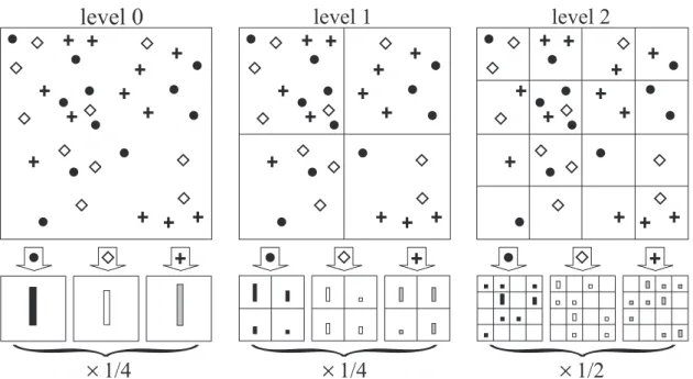
2.7 Example of a three-level pyramid . . . 18

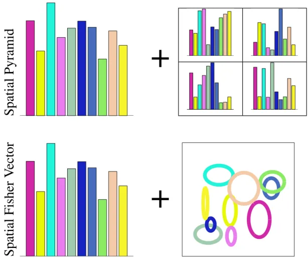
2.8 Comparison of SPM and SFV . . . 20

2.9 Images that NBNN has difficulty distinguishing . . . 21

2.10 Example of using a kernel to map data into a higher dimensionality space . . . . 23

2.11 Example pictures of the fifteen scene dataset . . . 24

2.12 Classification results for the SUN database . . . 26

4.1 Images in the SUN Database with disputable labels . . . 38

5.1 The SVM misclassification penalty parameter . . . 50

5.2 Impact of number of training images in classification accuracy . . . 51

6.1 Effect of humans on the foreground of an image . . . 57

LIST OF FIGURES

List of Tables

2.1 Classification results for the fifteen scene dataset . . . 25

4.1 Classification results where mean per-class accuracy is better . . . 36

4.2 Default settings used during the experiments . . . 37

5.1 Classification results for different types of descriptors . . . 41

5.2 Blurring images before extracting descriptors . . . 42

5.3 Impact of scaling images before feature extraction . . . 43

5.4 Using colour information during descriptor extraction . . . 44

5.5 Impact of scale and spacing of SIFT descriptors . . . 45

5.6 Transforming descriptors using Hellinger kernel . . . 46

5.7 Reducing dimensionality of a SIFT descriptor with size 128 . . . 46

5.8 The impact of codebook size in the Fisher framework . . . 47

5.9 The impact of codebook size when using Bag-of-Words . . . 47

5.10 Using spatial information with Bag-of-Words . . . 48

5.11 Differences between linear and non-linear SVM classifiers . . . 49

5.12 Settings used to achieve the best accuracy . . . 52

5.13 Confusion matrix for the best results . . . 52

5.14 Settings used to achieve better speed . . . 53

5.15 Confusion matrix for the balanced results . . . 53

5.16 Confusion matrix for the 15-scene dataset merged into two classes . . . 54

LIST OF TABLES

Abbreviations

CENTRIST CENsus TRansform hISTogram CUDA Compute Unified Device Architecture EXIF Exchangeable Image File

GPS Global Positioning System GPU Graphics Processing Unit HOG Histogram of Oriented Gradients HSV Hue, Saturation, Value

JSON JavaScript Object Notation kNN k-Nearest Neighbours LBP Local Binary Pattern

NBNN Naive Bayes Nearest Neighbour OpenCL Open Computing Language PCA Principal Component Analysis RGB Red, Green, Blue

SIFT Scale-Invariant Feature Transform SIMD Single Instruction, Multiple Data SFV Spatial Fisher Vectors

SPM Spatial Pyramid Matching SVM Support Vector Machine

UNEP United Nations Environment Programme WCMC Word Conservation Monitoring Centre

Chapter 1

Introduction

Decision-makers responsible for the monitoring and legislation of issues related to biodiversity and world conservation require data and expert knowledge on which to base their decisions.

This is where UNEP World Conservation Monitoring Centre comes in, as it is their mission to ‘evaluate and highlight the many values of biodiversity and put authoritative biodiversity know-ledge at the centre of decision-making’ (UNEP-WCMC2013).

With the objective of further expanding the range of information they can provide, UNEP-WCMC is also experimenting with automated data gathering and crowd-sourcing.

1.1

Context and Motivation

UNEP World Conservation Monitoring Centre, with data gathering and analysis as the core of their mission, described two different situations that could be improved with the use of computer vision and image processing techniques. Both of these scenarios, described in the following sections, refer to the same problem in their core, which is one of detecting nature in pictures.

1.1.1 Protected Planet

Protectedplanet.net is an interactive website that uses ‘Citizen Science’ to boost the global interest in protected areas. This means users are encouraged to find and improve information on protected areas around the world. This information ranges from their description and points of interest to pictures which can be shared and scored by the users for each of the protected areas of our planet. Figure1.1shows the appearance of the website.

To ensure the correctness of the information available in the website, all information submitted by users is curated by the the Protected Areas Programme’s staff at UNEP-WCMC. This manual process incurs in extra costs and carries a degree of subjectivity on what does and does not get accepted.

When dealing with user-submitted images, in order to reduce the costs and decrease the sub-jectivity of the review process, an automated solution, supported by computer vision and image processing techniques is ideal.

Introduction

(a) Main page (b) Protected area details

Figure 1.1: Screen captures of the protectedplanet.net website

1.1.2 Mapping Natural Areas

Websites like Flickr and Panoramio allow users to share geotagged images. The image’s location can be either obtained directly from the image by using Exchangeable Image File format (EXIF) tags, or provided manually by the user.

By using an image’s location and identifying whether it represents a natural scene or a man-made one, it is possible to determine the degree of naturalness on a particular location and time.

Processing a large number of images can fuel the creation of a map that identifies which areas of the Earth have been affected by human interference and which are still in their natural state. If an image’s timestamp is also taken into account, then it is also possible to see the evolution of these man-made and natural areas.

This information is important to legislators and decision-makers as it provides them with de-tails regarding possibly problematic areas that may require intervention or to study the impact of other actions that may have been taken previously. Another use for this data is that it can also be cross-referenced with information about protected areas to evaluate their effectiveness.

1.2

Problem Definition

The problem to be solved consists of the definition and implementation of a tool that is capable of automatically evaluating a picture and classifying it into one of two classes: natural or man-made. In order to improve its acceptance as a replacement for manual evaluation, the tool should always output its confidence rating regarding the decision made, allowing for the final verdict to be deferred to a human operator when a low confidence decision is reached.

For an automation of the entire classification process, the tool should be able to be easily in-tegrated into existing applications, such as the protectedplanet.net website, or to be plugged into a new application that may require the same kind of data evaluation, allowing for its parametrization for more effective image processing in each of these different contexts.

Introduction

1.3

Main Goals

The main goals of this work can be summarized as follows:

• Compare the usefulness of several competing state-of-the-art scene classification algorithms

when applied to the task of determining the degree of naturalness of an image.

• Provide an open-source, easy to extend framework for automated scene classification and

algorithm evaluation.

• Evaluate the computational cost of the implemented techniques and the influence of changes

in their parameters in said cost and analyse any trade-offs between speed and accuracy.

• Analyse the implemented algorithm’s ability to generalize the information gathered from

training on one dataset and applying it to a different data source.

• Test the framework’s ability to cope with irrelevant information that may appear on images,

such as the presence of humans in pictures.

• Provide a detailed description of all settings used to during the experiments to allow for easy

reproduction of the results.

1.4

Document Structure

Chapter2reviews the current state-of-the-art techniques used in the scene classification area. An overview of each technique, as well as its possible advantages and shortcomings in comparison to other alternatives are also presented. Always taking into account the goals of this work, this chapter also identifies some of the knowledge gaps in the literature.

Details about the developed framework are presented in chapter 3. The main tasks that are required of such framework are listed, as well as other optional improvements that were also added. External libraries and details about their inclusion in the project are also described here.

Chapter4describes the procedure used to execute all of the reported experiments. Information about the dataset and how it was built, as well as all parameters is also included. The main limitations of the experiments that were performed are also detailed in this section.

The results of the experiments are presented in chapter5. The algorithms identified in chapter2

are compared, as well as their parameters, reporting their impact on the classification performance and computational cost. Taking into account these experiments, an overview of the impact of optimizing the framework’s parameter for both speed and accuracy is provided.

Chapter6goes through the goals of this work, analysing and discussing their viability based on the results of the experiments.

Introduction

Chapter 2

Scene Classification

Scene classification, or scene recognition, refers to the problem of automatically assigning a label to an image among a set of semantic categories (e.g. forest, mountain, and street) (Wu and Rehg

2011; Zhou, Zhou and Hu2013). The applications for scene classifications range from acquir-ing context for object recognition (Torralba2003), to content-based image indexing and retrieval (Vogel and Schiele2007), and to robot and vehicle navigation (Wu and Rehg2011).

One can define the problem of detecting whether the view represented in a picture corresponds to a natural or a man-made scene as a subset of the scene classification problem. In fact, determ-ining the degree of naturalness of a picture is a part of the ‘Spatial Envelope’ technique proposed by Oliva and Torralba (2001) for scene classification.

The act of classifying an image has three major components. The first one is the extraction of a set of features from the image, which is detailed in sections2.1 to2.3. Then, a representation of the image is created, using the process outlined in sections2.4to2.6. The final part is using a machine learning technique to classify the images, as described in sections2.7and2.8.

2.1

Features

A feature of an image is a representation, characteristic or property of that image (Boutell, Brown and Luo2002).

There are several features that can be used for scene classification, such as colour, texture, filter outputs and gradients.

2.1.1 Colour

Computers can represent colours in many different formats. Each of these may provide different in-variance properties, such as light colour or light intensity changes and shifts, to image descriptors, when used as part of an image classification framework. Some of the most popular are RGB, Opponent and HSV (Van de Sande, Gevers and Snoek2010).

RGB is the most common colour space used by computer images since it is the same repres-entation required by computer screens. It uses three channels corresponding to the intensity of the

Scene Classification

colours red, green and blue. These three components are added together using an additive colour model in order to get the final colour.

The opponent colour space corresponds to the Principal Component Analysis of the RGB colour representation on a set of images. The transformation described in eq. (2.1), obtained by using PCA on a set of natural images, can be used to decorrelate the colour components of a set of images (Boutell, Brown and Luo2002).

   O1 O2 O3    =     R_√−G 2 R+G_√−2B 6 R+G+B_√ 3     (2.1)

HSV is another way to represent colours, by using the hue, saturation and value components. While the properties of this model make for a good colour picker system and is commonly used in image editing software, it has also been successfully used in the field of computer vision (Bosch, Zisserman and Muñoz2008).

2.1.2 Texture

The texture of an image patch refers to an object’s surface and structural properties. While the direct application of textural properties has been used to distinguish between different material and textile patterns, such as in the work by Ojala, Pietikainen and Maenpaa (2002), most works in scene classification opt for simpler properties to describe an image, such as gradients, described in section2.1.4.

2.1.3 Filter Outputs

Several signal processing filters can be applied to image processing as well. Among these, the Fourier transform and Gabor filters are the most common. Gabor filters can be used as an edge detection tool as they can filter an image’s components that are oriented in a certain angle. The Fourier transform, on the other hand, decomposes a signal into its sinusoidal components. When these two filters are combined, they can be used to determine the frequency of a signal in an image for a given orientation.

2.1.4 Gradients

Gradients can be used to determine orientations and borders of objects and shapes. There are sev-eral ways of representing gradients, ranging from simple binary representations, saying whether the value increased or decreased between two points, to more complex representations that calcu-late the gradient intensity and orientation.

Gradients are the most common features used by descriptors in scene classification (Lowe

2004; Dalal and Triggs2005).

Scene Classification

2.2

Descriptors

In order to turn the features described in the previous chapter into a more tractable representa-tion, several descriptors have been proposed for image processing. These descriptors attempt to move away from pixel representations and to provide a description closer to the image semantics (Boutell, Brown and Luo2002). There are several desirable properties in a descriptor for its use in scene classification (Wu and Rehg2011). Descriptors should allow for a holistic representation of the scene, since a global view of an image can give more details about a scene than informa-tion about its components. They should be able to capture structural properties of a scene, such as shapes, flat surfaces, and tiles without getting distracted by detailed textural information. The descriptor should also be generalizable, allowing for the comparison of vastly different visual representations of the same semantic concept.

The next sections describe the most often used descriptors that achieve good results for scene classification: Gist, SIFT, HOG, LBP, and CENTRIST. Figure2.1shows the results of the applic-ation of some descriptors to an example picture.

(a) Original picture (b) Gist descriptor

(c) SIFT descriptor (d) HOG descriptor

Scene Classification

2.2.1 Gist

First described by Oliva and Torralba (2001) this descriptor attempts to represent spatial structures by using a ‘Discrete Fourier Transform’ to calculate the power spectra of an image and ‘Prin-cipal Component Analysis’ to filter the frequencies used to describe the image. This allows for a representation of the image that uses exclusively global features.

While an important work, as a pioneer for scene recognition without segmenting or recogniz-ing local objects, its results have been surpassed by state-of-the-art approaches.

2.2.2 SIFT

‘Scale-Invariant Feature Transform’ is one of the most used descriptors in the scene classification literature (Bosch, Muñoz and Martí2007; Wu and Rehg2011). It was proposed by Lowe (2004) as a way to extract features that could be used to match different views of an object or scene.

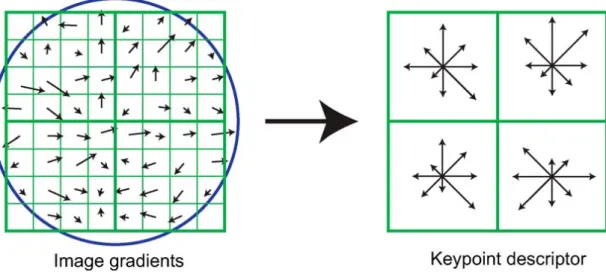
Once the point where the descriptor will be extracted from has been determined, using one of the techniques described in section2.3, including its scale and rotation, the SIFT can be calculated for that point. This is done by creating an histogram of gradient intensity and orientations, where Lowe (2004) uses a 4 by 4 grid of bins and 8 gradient orientations, resulting in a 4× 4 × 8 = 128 element feature vector, as exemplified in fig.2.2. Each of these bins is weighted using a Gaussian window, meaning that bins further away from the descriptor centre are weighted less than the ones closer to the centre.

Distinctive Image Features from Scale-Invariant Keypoints

101

Figure 7. A keypoint descriptor is created by first computing the gradient magnitude and orientation at each image sample point in a region around the keypoint location, as shown on the left. These are weighted by a Gaussian window, indicated by the overlaid circle. These samples are then accumulated into orientation histograms summarizing the contents over 4x4 subregions, as shown on the right, with the length of each arrow corresponding to the sum of the gradient magnitudes near that direction within the region. This figure shows a 2× 2 descriptor array computed from an 8× 8 set of samples, whereas the experiments in this paper use 4 × 4 descriptors computed from a 16 × 16 sample array.

6.1.

Descriptor Representation

Figure 7 illustrates the computation of the keypoint

de-scriptor. First the image gradient magnitudes and

ori-entations are sampled around the keypoint location,

using the scale of the keypoint to select the level of

Gaussian blur for the image. In order to achieve

ori-entation invariance, the coordinates of the descriptor

and the gradient orientations are rotated relative to

the keypoint orientation. For efficiency, the gradients

are precomputed for all levels of the pyramid as

de-scribed in Section 5. These are illustrated with small

arrows at each sample location on the left side of

Fig. 7.

A Gaussian weighting function with

σ equal to one

half the width of the descriptor window is used to

as-sign a weight to the magnitude of each sample point.

This is illustrated with a circular window on the left

side of Fig. 7, although, of course, the weight falls

off smoothly. The purpose of this Gaussian window is

to avoid sudden changes in the descriptor with small

changes in the position of the window, and to give less

emphasis to gradients that are far from the center of the

descriptor, as these are most affected by misregistration

errors.

The keypoint descriptor is shown on the right side

of Fig. 7. It allows for significant shift in gradient

po-sitions by creating orientation histograms over 4

× 4

sample regions. The figure shows eight directions for

each orientation histogram, with the length of each

ar-row corresponding to the magnitude of that histogram

entry. A gradient sample on the left can shift up to 4

sample positions while still contributing to the same

histogram on the right, thereby achieving the objective

of allowing for larger local positional shifts.

It is important to avoid all boundary affects in which

the descriptor abruptly changes as a sample shifts

smoothly from being within one histogram to another

or from one orientation to another. Therefore,

trilin-ear interpolation is used to distribute the value of each

gradient sample into adjacent histogram bins. In other

words, each entry into a bin is multiplied by a weight of

1

−d for each dimension, where d is the distance of the

sample from the central value of the bin as measured

in units of the histogram bin spacing.

The descriptor is formed from a vector containing

the values of all the orientation histogram entries,

cor-responding to the lengths of the arrows on the right side

of Fig. 7. The figure shows a 2

× 2 array of

orienta-tion histograms, whereas our experiments below show

that the best results are achieved with a 4

× 4 array of

histograms with 8 orientation bins in each. Therefore,

the experiments in this paper use a 4

× 4 × 8 = 128

element feature vector for each keypoint.

Finally, the feature vector is modified to reduce the

effects of illumination change. First, the vector is

nor-malized to unit length. A change in image contrast in

which each pixel value is multiplied by a constant will

multiply gradients by the same constant, so this contrast

change will be canceled by vector normalization. A

brightness change in which a constant is added to each

image pixel will not affect the gradient values, as they

are computed from pixel differences. Therefore, the

de-scriptor is invariant to affine changes in illumination.

However, non-linear illumination changes can also

oc-cur due to camera saturation or due to illumination

Figure 2.2: SIFT descriptor example using a 2 by 2 patch (Lowe2004)

Once the descriptor has been calculated, it is normalized using a two step normalization pro-cess. First, the descriptor is L2-normalized, then the values of all bins are clamped to a maximum of 0.2, and the descriptor is, once again, normalized with L2-norm. These operations aim to reduce the effects of illumination changes.

A more recent approach, used by Vedaldi and Fulkerson (2008) employs an approximation, which instead of using a Gaussian window to weight the bins, uses a flat window which is then

Scene Classification

reweighed by the average Gaussian of all bins. This speeds up the calculation of the descriptor by an order of magnitude, with little or no impact in the classification results.

The strengths of the SIFT descriptor are related to its invariance to scale and rotation of each feature. It is also robust against changes in distortion, viewpoint, noise, and illumination.

2.2.3 HOG

Originality described by Dalal and Triggs (2005) for human detection, the ‘Histogram of Oriented Gradients’ descriptor has been shown to perform very well in scene classification tasks (Xiao et al.

2010; Zhou, Zhou and Hu2013).

This descriptor represents a picture by calculating an histogram of the orientation of gradients for a small patch of the image. In order to calculate the histograms, a number of orientations is defined, usually ranging from 4 to 16, and the intensity of the gradients for each of the orientations is calculated.

2.2.4 LBP

‘Local Binary Patterns’ is a grey scale and rotation invariant descriptor used for uniform pattern detection (Ojala, Pietikainen and Maenpaa2002).

LBP works by comparing a central, anchor point, to a number of points along a circle of a pre-defined radius around the anchor. This comparison is a purely binary decision on whether the sampled point is larger than the central value or not, which provides a great invariance to light intensity changes. When the position of one of the points does not match with a pixel, interpolation is used to retrieve the image information.

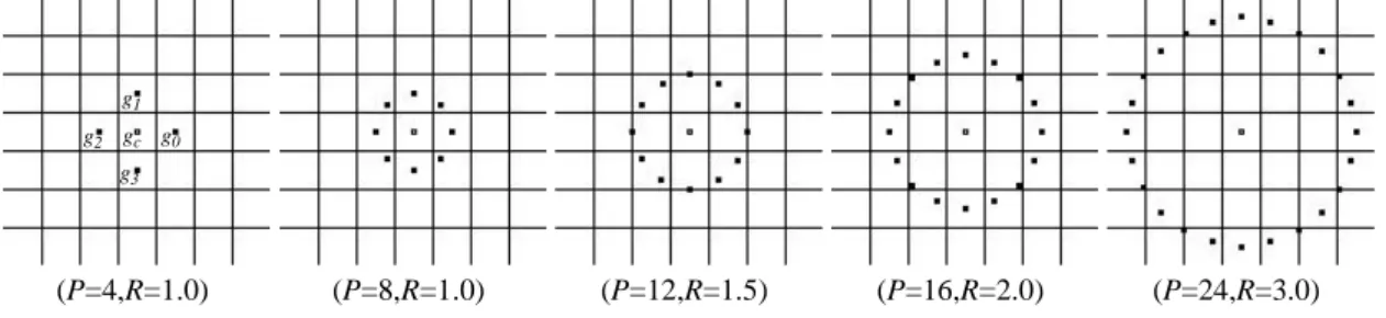
The number of points and the radius of the circle are the only two parameters of this descriptor, which is represented as a subscript of the LBP name, starting with the number of points and followed by the radius. LBP8,1represents an LBP descriptor with 8 points sampled along a circle

of radius 1. See fig.2.3for some examples of different sized LBP descriptors.

2.1 Achieving Gray Scale Invariance

As the first step towards gray scale invariance we subtract, without losing information, the gray value of the center pixel (g_c) from the gray values of the circularly symmetric neighbor-hood g_p (p=0,...,P-1) giving:

Next, we assume that differences g_p-g_c are independent of g_c, which allows us to factorize Eq.(2):

In practice an exact independence is not warranted, hence the factorized distribution is only an approximation of the joint distribution. However, we are willing to accept the possible small loss in information, as it allows us to achieve invariance with respect to shifts in gray scale. Namely, the distribution t(g_c) in Eq.(3) describes the overall luminance of the image, which is

unrelated to local image texture, and consequently does not provide useful information for tex-ture analysis. Hence, much of the information in the original joint gray level distribution (Eq.(1)) about the textural characteristics is conveyed by the joint difference distribution [29]:

This is a highly discriminative texture operator. It records the occurrences of various pat-terns in the neighborhood of each pixel in a P-dimensional histogram. For constant regions, the differences are zero in all directions. On a slowly sloped edge, the operator records the highest difference in the gradient direction and zero values along the edge, and for a spot the differ-ences are high in all directions.

Fig. 1. Circularly symmetric neighbor sets for different (P,R). (P=8,R=1.0) (P=4,R=1.0) (P=12,R=1.5) (P=16,R=2.0) (P=24,R=3.0) gc g1 g2 g3 g0 T = t g( _c,g₀–g_c,g₁–g_c, ,... g_P–1–g_c) (2) T≈t g( )_c t g( ₀–g_c,g₁–g_c, ,... g_P–1–g_c) (3) T≈t g( ₀–g_c,g₁–g_c, ,... g_P–1–g_c) (4)

Figure 2.3: Multiple LBP configurations (Ojala, Pietikainen and Maenpaa2002)

Further improvements are also proposed in order to achieve rotation invariance, by repeatedly applying a circular bit-wise shift, with the objective of minimizing the descriptor value. What this achieves is a descriptor that only cares about the general shape of the pattern being represented, as as any rotation to that pattern will be cancelled by the bit-wise shift.

Scene Classification

Another improvement proposed by the authors is the removal of descriptors that contain more than two bitwise 0/1 changes. While this operation filters a large number of descriptors, they only account for 10% of the total descriptors in the texture images used by Ojala, Pietikainen and Maenpaa (2002), and thus do not provide enough data for reliable image comparison.

The main advantage of this descriptor is its very small size, which can usually fit in a single integer value. In turn, this means that LBP descriptors can be extracted very densely, up to a descriptor for every pixel in the image, thus reducing the amount of information that may be discarded by other proposed descriptors.

2.2.5 CENTRIST

The newest descriptor, named ‘CENsus TRansform hISTogram’, was proposed by Wu and Rehg (2011) and was designed for place and scene recognition tasks. It is a simplification of the LBP descriptor, corresponding to the LBP8,1, but using a scan-line approach to order the bits instead of

the circular extraction used by Ojala, Pietikainen and Maenpaa (2002).

This descriptor boasts its lack of parameters to tune, its fast evaluation speed and ease of implementation. The results presented for the fifteen scene dataset, described in section2.8.1, are on par or superior to those of the more popular SIFT descriptor.

2.3

Extraction Method

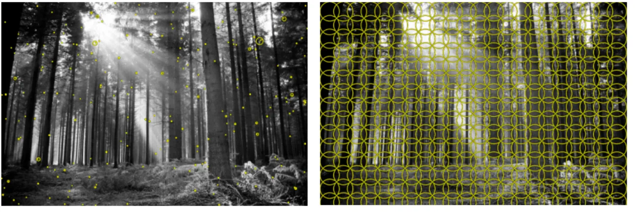
There are several techniques that can be applied to feature extraction when using the previous descriptors. Figure2.4exemplifies some of the extraction techniques which will be explained in detail in the following sections.

(a) Points of interest (b) Dense grid

Figure 2.4: Two distinct extraction techniques

2.3.1 Sparse

SIFT descriptors, as defined by Lowe (2004), use a technique to discover points of interest. These points of interest are usually corners or edge points with high gradients which contain useful

Scene Classification

information that can be used to compare objects or scenes taken from different viewpoints. The descriptors are then extracted for each of these points of interest.

In order to determine the points of interest a technique called difference-of-Gaussians is used. To apply this technique the image is blurred using several different Gaussian levels and the res-ulting images are subtracted from each other. The points corresponding to the extrema of these differences are then used as interest points.

2.3.2 Dense

Alternatively, features can be extracted on a dense grid. This involves the division of the image into small patches, wherein a feature is extracted, whether or not the patch contains any gradient or other useful characteristic. The distance between each of these patches, measured in pixels, can also be called ‘descriptor spacing’.

For scene classification, dense extraction of features has been shown to improve the results, since the lack of any significant features can be an important piece of information by itself (Fei-Fei and Perona2005).

It has also been shown that overlapping the patches where the features are extracted can further improve the scene classification results (Bosch, Zisserman and Muñoz2008).

2.3.3 Multi-resolution

The multi-resolution technique involves the extraction of features on multiple resolution levels of the image (Wu and Rehg2011; Zhou, Zhou and Hu2013). It requires the extraction of features, using either a dense or sparse approach, followed by the halving of the size of the image. This process can be repeated several times, resulting in several sets of features, one for each different resolution. Zhou, Zhou and Hu (2013) identify the use of three levels as an ideal amount of image scales to use in the context of scene classification.

When combined with dense feature extraction, the size of the patch is also scaled down, in order to gather roughly the same amount of descriptors for each image resolution.

An alternative to scaling an image directly is to extract the descriptors in multiple scales, which simulates the image resizing. Scaling descriptors involves calculating the descriptor using a larger or smaller number of pixels around a central point, which results in a descriptor that summarizes more or less information, respectively. Several works have used this technique, improving the classification results when compared to using a single scale descriptor (Bosch, Zisserman and Muñoz 2008; Perronnin, Sánchez and Mensink 2010; Krapac, Verbeek and Jurie 2011). The implementation of this multi-scale feature extraction may differ regarding the placement of the different scale descriptors, having some authors opted for concentric descriptor extraction and others for no alignment between different scales.

Scene Classification

2.4

Descriptor Transformation

2.4.1 Hellinger Kernel

Many of the intermediate representations presented in the following section require the compar-ison of descriptors. To achieve this, techniques such as k-means traditionally use L2 distance, also known as Euclidean distance. Using the Euclidean distance has been shown to be less than ideal for the comparison of histogram representations. As descriptors such as SIFT and HOG are his-tograms themselves better results can be achieved if a more adequate distance comparison is used (Arandjelovic and Zisserman2012).

A simple way to use another distance measure without rewriting the image processing pipeline is to apply a mapping function to the descriptors. Several approximate mappings for kernels have been proposed by Vedaldi and Zisserman (2010) but one in particular is very useful for descriptor transformation, as it can be applied in place, without changing the size of the descriptor, which is the Hellinger kernel.

The Hellinger mapping, also called RootSIFT when applied to SIFT descriptors, can be cal-culated in two simple steps. The first step it to normalize the descriptor using L1 distance, also known as Manhattan distance. Then, each element of the descriptor is replaced by its square root. This simple and cheap to compute transformation has been shown to greatly improve the classification results in scene and object classification tasks (Arandjelovic and Zisserman 2012; Garg, Chandra and Jawahar2012).

2.4.2 Principal Component Analysis

Principal Component Analysis (PCA), is a technique that can be used to decorrelate and reduce dimensionality of data. While using PCA to reduce the dimensionality of data results in loss of information, this analysis maximizes the compression to loss ratio (Smith2002).

The first step of performing PCA on a dataset is to center the data so it has mean zero. This allows for the computation of the covariance matrix, which is a square matrix with side equal to the number of dimensions of the data and represents how likely it for the data in one dimen-sion to change when the data in another dimendimen-sion also changes. Calculating the eigenvectors and the corresponding eigenvalues of this covariance matrix allows the dimensions to be trans-formed according to their relevance and importance for the representation of data, as the higher the eigenvalue, the higher the significance of the respective eigenvector. In order to reduce an

N-dimensional data into a D-dimensional representation it has to simply be multiplied by a matrix

containing the D N-dimensional eigenvectors with the highest eigenvalues.

PCA can be combined with other encoding techniques described in this chapter by using it to process and reduce the dimensionality of the descriptors before using them as one would do with any other descriptor.

Scene Classification

2.5

Intermediate Representations

Some of the proposed techniques for scene classification use the extracted features to directly describe an image, such as is the case with NBNN described in section2.7.1. However, new devel-opments in the scene classification literature have shown that using an intermediate representation of the extracted features can boost the accuracy of the scene classification task (Bosch, Muñoz and Martí2007).

2.5.1 Bag-of-Words Representation

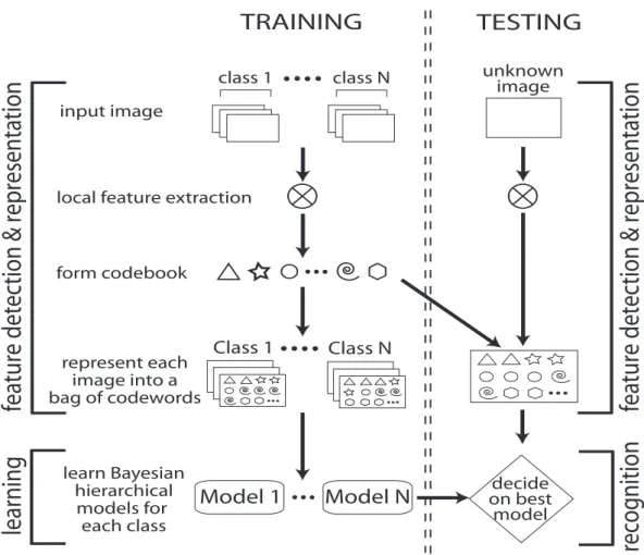
The Bag-of-Words technique, used for text analysis and categorization, has shown excellent per-formance when applied to scene classification. This technique, as described by Fei-Fei and Perona (2005), is named as Bag-of-Codewords, Bag-of-Features or Bag-of-Visual-Words in the literature. Bag-of-Codewords abstracts the representation of an image by creating a codebook of features. This codebook is formed by extracting a large number of features from a diverse set of images and then grouping those features into a smaller, pre-defined number of codewords using clustering techniques. A diagram explaining this process can be found in fig.2.5

and expensive, and because expert-defined labels are

some-what arbitrary and possibly sub-optimal.

Much can also be learnt from studies for classifying

dif-ferent textures and materials [10, 5, 16]. Traditional texture

models first identify a large dictionary of useful textons (or

codewords). Then for each category of texture, a model is

learnt to capture the signature distribution of these textons.

We could loosely think of a texture as one particular

in-termediate representation of a complex scene. Again, such

methods yield a model for this representation through

man-ually segmented training examples. Another limitation of

the traditional texture model is the hard assignment of one

distribution for a class. This is fine if the underlying images

are genuinely created by a single mixture of textons. But

this is hardly the case in complex scenes. For example, it

is not critical at all that trees must occupy 30% of a suburb

scene and houses 60%. In fact, one would like to recognize

a suburb scene whether there are many trees or just a few.

The key insights of previous work, therefore, appear to

be that using intermediate representations improves

perfor-mance, and that these intermediate representations might be

thought of as textures, in turn composed of mixtures of

tex-tons, or codewords. Our goal is to take advantage of these

insights, but avoid using manually labeled or segmented

im-ages to train the system, if possible at all. To this end, we

adapt to the problems of image analysis recent work by Blei

and colleagues [1], which was designed to represent and

learn document models. In this framework, local regions

are first clustered into different intermediate themes, and

then into categories. Probability distributions of the local

regions as well as the intermediate themes are both learnt in

an automatic way, bypassing any human annotation. No

su-pervision is needed apart from a single category label to the

training image. We summarize our contribution as follows.

• Our algorithm provides a principled approach to learning

rel-evant intermediate representations of scenes automatically

and without supervision.

• Our algorithm is a principled probabilistic framework for

learning models of textures via codewords (or textons) [5,

16, 10]. These approaches, which use histogram models of

textons, are a special case of our algorithm. Given the

flex-ibility and hierarchy of our model, such approaches can be

easily generalized and extended using our framework.

• Our model is able to group categories of images into a

sensi-ble hierarchy, similar to what humans would do.

We introduce the generative Bayesian hierarchical model

for scene categories in Section 2. Section 3 describes our

dataset of 13 different categories of scenes and the

experi-mental setup. Section 4 illustrates the experiexperi-mental results.

TRAINING

TESTING

fe

ature detec

tion & representation

learning

fe

ature detec

tion & representation

recognition

unknown image class 1 class N input image

Model 1

Model N

learn Bayesian hierarchical models for each class

local feature extraction

form codebook Class 1 Class N represent each image into a bag of codewords decide on best model

Figure 2.

Flow chart of the algorithm.

2. Our Approach

Fig.2 is a summary of our algorithm in both learning and

recognition. We model an image as a collection of local

patches. Each patch is represented by a codeword from a

large vocabulary of codewords (Fig.4). The goal of learning

is to achieve a model that best represents the distribution of

these codewords in each category of scenes. In recognition,

therefore, we first identify all the codewords in the unknown

image. Then we find the category model that fits best the

distribution of the codewords of the particular image.

Our algorithm is modified based on the Latent

Dirich-let Allocation (LDA) model proposed by Blei et al. [1].

We differ from their model by explicitly introducing a

cat-egory variable for classification. Furthermore, we propose

two variants of the hierarchical model (Fig.3(a) and (b)).

2.1

Model Structure

It is easier to understand the model (Fig.3(a)) by going

through the generative process for creating a scene in a

spe-cific category. To put the process in plain English, we begin

by first choosing a category label, say a mountain scene.

Given the mountain class, we draw a probability vector that

will determine what intermediate theme(s) to select while

generating each patch of the scene. Now for creating each

patch in the image, we first determine a particular theme

out of the mixture of possible themes. For example, if a

“rock” theme is selected, this will in turn privilege some

codewords that occur more frequently in rocks (e.g. slanted

lines). Now the theme favoring more horizontal edges is

chosen, one can draw a codeword, which is likely to be a

horizontal line segment. We repeat the process of drawing

both the theme and codeword many times, eventually

form-ing an entire bag of patches that would construct a scene of

mountains. Fig.3(a) is a graphical illustration of the

gener-Figure 2.5: Diagram of the bag-of-codewords technique (Fei-Fei and Perona2005) 13

Scene Classification

Once each descriptor has been assigned to one of the codewords, an histogram of codeword occurrences is built for the entire image. It is this histogram that forms the basis of the comparison between images.

2.5.1.1 k-means Clustering

One of the most popular techniques used to cluster the extracted features of the images is k-means (Gao, Tsang and Chia 2013). This technique takes a number of representative features and at-tempts to calculate a pre-defined number of clusters, minimizing the distance between each cluster centroid and the features assigned to it.

This can be formulated as the solution to the problem described by eq. (2.2) (Yang et al.2009), where X = [x1, . . . , xM]∈ RM×Dis a set of D-dimensional descriptors, V = [v1, . . . , vK] are the K

cluster centres to be determined by the algorithm, and∥ · ∥2is the L2-norm of the vectors: min V M

∑

m=1 min k=1...K∥ xm− vk∥ 2 _(2.2)

The k-means algorithm solves this problem by using an iterative, two-step process, as de-scribed in algorithm2.1. The first part of the algorithm is an ‘assignment step’, where each feature is assigned to its nearest cluster centre. This is followed by an ‘update step’, where new cluster centres are determined by averaging the assignments to each cluster. The entire process is then repeated until the centres do not change between two consecutive iterations.

Algorithm 2.1k-means clustering algorithm Input:

X = [x1, . . . , xM] ◃ data to be clustered

K ◃ number of clusters

Output:

V = [v1, . . . , vK] ◃ cluster centres

D(x) = centre closest to x ◃ centre assignments

V ← initial cluster centres ◃ e.g. random selection of X

repeat

for all xi∈ X do

D(xi)← argmin_{j∈{1,...,K}}distance(xi,Vj) ◃ find the closest centre

end for

for i =1→ K do

vi← centroid of {x|D(x) = i} ◃ update cluster centres

end for

until V does not change

The main advantages of this algorithm is that not only is it very simple to implement, but it also quickly converges to a local optimum, which means it can be interrupted before fully converging and still return usable cluster centres.

On the other hand, as a clustering technique, it does have several shortcomings. Due to the 14

Scene Classification

way k-means uses a simple L2-distance as a measure to find the closest cluster centres, it tends to generate equal sized clusters, which may not be the optimal encoding for the features. Its high dependency on the initial, randomly generated cluster centres, as well as its loss of information, in particular when considering the features closest to the cluster boundaries, are also are issues that must be considered when using this technique (Gao et al.2010).

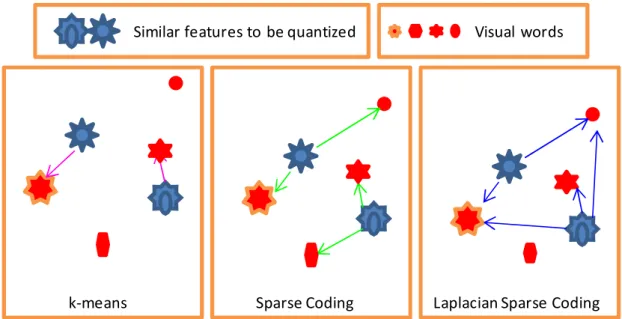
2.5.1.2 Sparse Coding

Newer alternatives have been proposed to form the codebook using a sparse-coding algorithm to allow for soft assignment of features (Gemert et al.2008). This means that each feature may be assigned to more than one cluster centroid. Figure2.6contrasts the different clustering techniques.

Local Features Are Not Lonely – Laplacian Sparse Coding for

Image Classification

Shenghua Gao, Ivor Wai-Hung Tsang,

Liang-Tien Chia, Peilin Zhao

School of Computer Engineering, Nanyang Technological University, Singapore

{gaos0004,IvorTsang,asltchia,zhao0106}@ntu.edu.sg

Abstract

Sparse coding which encodes the original signal in a

sparse signal space, has shown its state-of-the-art

perfor-mance in the visual codebook generation and feature

quan-tization process of BoW based image representation.

How-ever, in the feature quantization process of sparse coding,

some similar local features may be quantized into

differ-ent visual words of the codebook due to the sensitiveness of

quantization. In this paper, to alleviate the impact of this

problem, we propose a Laplacian sparse coding method,

which will exploit the dependence among the local features.

Specifically, we propose to use histogram intersection based

kNN method to construct a Laplacian matrix, which can

well characterize the similarity of local features. In

addi-tion, we incorporate this Laplacian matrix into the

objec-tive function of sparse coding to preserve the consistence

in sparse representation of similar local features.

Compre-hensive experimental results show that our method achieves

or outperforms existing state-of-the-art results, and exhibits

excellent performance on Scene 15 data set.

1. Introduction

Image classification is one of the fundamental

prob-lems in computer vision, which has attracted lots of

re-searchers’ attention these years. Many image

representa-tion models have been proposed for this problem, such as

Part-based model [

3

], Bag of Words(BoW) model [

18

], etc.

Amongst these models, BoW model has shown excellent

performance and been widely used in many real

applica-tions (such as image classification [

22

], image annotation

[

21

], image retrieval [

16

] and video event detection [

24

])

due to its robustness to scale, translation and rotation

vari-ance.

BoW image representation contains the following three

modules: (i) Region selection and representation; (ii)

Code-book generation and feature quantization; (iii) Frequency

histogram based image representation.

k-means Sparse Coding Laplacian Sparse Coding Similar features to be quantized Visual words

Figure 1. Feature Quantization strategies for different methods. In

k-means, each feature is only assigned to one clustering center; In

sparse coding, features are automatically assigned to the centers

that can optimally reconstruct this feature, but it is sensitive to

feature variance. In Laplacian sparse coding, similar features are

not only assigned to optimally-selected cluster centers, but we also

guarantee the selected cluster centers are also similar. Therefore,

Laplacian sparse coding is more robust for feature quantization.

In these three modules, codebook generation and feature

quantization are the most important and govern the quality

of image presentation. Codebook, whose entries are termed

as visual words, is a collection of basic patterns used to

re-construct the input local features. Usually hard assignment

method, such as k-means is adopted to generate the

code-book, and kNN is used to assign each local feature to the

visual words. However, such method may cause severe

in-formation loss [

1

] by assigning each visual feature to only

one visual word, especially for those features located at

the boundary of several visual words. Thereafter, soft

as-signment [

16

,

19

] is introduced to assign each feature to

more than one visual words. However, the way of assigning

weight to the visual words and the number of visual words

to be assigned for each visual feature are not trivial to be

determined.

One evident drawback in BoW model is the spatial

in-formation loss. To overcome this, Lazebnik et al.[

8

]

ex-tended the BoW model with Spatial Pyramid Matching

Ker-nel (SPM) by exploiting the spatial information of location

regions. More specifically, each image is partitioned into

increasingly finer sub-regions and Pyramid Match Kernel

[

4

] is used to compare corresponding sub-regions. Many

work [

8

,

24

,

25

] have shown the effectiveness of SPM in

3555

978-1-4244-6985-7/10/$26.00 ©2010 IEEE

Figure 2.6: Clustering techniques for the codebook creation (Gao et al.2010)

The sparse coding problem can be seen as a generalization of the hard clustering problem defined in eq. (2.2). Equation (2.2) can be transformed into a matrix factorization problem, having

U = [u1, . . . , uK] represent the cluster membership, ∥ · ∥ is the L2-norm of a vector, | · | is the

L1-norm, and Card(x) is the number of non-zero elements in x: min U,V M

∑

m=1 ∥ xm− umV∥2

subject to: Card(um) = 1,|um| = 1,um≽ 0,∀m

(2.3) By relaxing the Card(um) = 1 requirement we can turn the problem into one of soft assignment.

In order to limit the number of non-zero assignments, a term containing the L1-norm um can

be introduced. The importance of this term, which basically represents the sum of the cluster membership assignments, can be tweaked using the factorλ, resulting in the following formulation

Scene Classification for the sparse coding problem (Yang et al.2009):

min U,V M

∑

m=1 ∥ xm− umV ∥2_+λ|um| subject to: ∥ vk∥≤ 1,∀k = 1,2,...,K (2.4) An improvement to the Sparse Coding technique has been proposed by Gao et al. (2010), called Laplacian Sparse Coding, who identify that descriptors that are similar amongst themselves sometimes end up being encoded using a completely different set of codewords. To fix this, they introduce the use of a Laplacian matrix, which characterizes the similarity of local features, in order to ensure similar features are encoded into similar codewords.

This category of techniques, which relax the descriptor assignment into codewords, resulting in less data loss, shows significantly better results over the standard k-means when applied to scene classification (Gemert et al.2008; Gao et al.2010). This is explained by Boiman, Shechtman and Irani (2008) who argue that, while feature quantization does significantly decrease the feature dimensionality, it also degrades the discriminative power of descriptors. As such, a representation that is closer to the original descriptor, such as Sparse Coding, will result in a more discriminative representation.

2.5.2 Fisher Kernel

The Fisher Kernel is a framework which combines both generative and discriminative approaches to characterise a signal. For the image classification problem, this framework can be adapted by considering an image as the input signal and by using a visual vocabulary as the generative model. For this vocabulary, Gaussian Mixture Models, or GMMs for short, can be used to represent the distribution of low-level features in images (Perronnin and Dance2007).

GMMs are built by taking a number of descriptors and adapting a pre-defined number of Gaussians to that data. They do this with the help of an expectation-maximization algorithm which iteratively improves the fit between the gaussians and the data.

The kernel itself, which is used to compute the similarity between two Fisher vectors, can be computed using the following equation, where Fxis the Fisher vector for image x:

K(X ,Y ) = F_XTI−1FY (2.5)

I represents the Fisher information matrix. Since this matrix can have a very high dimension,

it is commonly replaced with a diagonal approximation (Krapac, Verbeek and Jurie2011). 2.5.2.1 Fisher Vector

The contents of the Fisher vector itself can change depending on what information is included during its calculation. If all information is used, which results in a more detailed representation and

Scene Classification

thus better classification results, it contains a total of K(1+2D) dimensions, where K is the number of keywords and D is the dimension of each descriptor (Perronnin and Dance2007). Of these dimensions, K correspond to the weights of each keyword, KD to the average of the descriptors assigned to a keyword, and another KD represent the standard deviation of those descriptors.

The biggest advantage this representation has over that of the Bag-of-Words technique is that, for the same codebook size, it results in a descriptor that is several orders of magnitude larger. This larger, more descriptive representation, allows for images to be classified using a simple linear classifier without any significant loss in performance. Section2.7provides additional information regarding classifiers.

2.5.2.2 Vector Normalization

Perronnin, Sánchez and Mensink (2010) determined that the Fisher vector representation contains some image-specific information. This means that two images containing the same subject but different amounts of background information, as is the case in pictures of the same subject in multiple scales, will result in different signatures. To reduce this problem, the Fisher vector can be normalized using L2-norm, allowing for better classification results. This is equivalent to replacing the classifier kernel with the following equation:

K(X ,Y )

√

K(X , X )K(Y,Y ) (2.6)

While using L2-normalization does improve the classification results, they can be further im-proved by combining it with another normalization technique. The need for another normaliza-tion process arises from the empirical observanormaliza-tion that a larger number of Gaussians will result in sparser Fisher vector representations. Perronnin, Sánchez and Mensink (2010) argue that L2-distance is a poor measure of L2-distance for sparse vectors and as such they propose the use of the transformation described in eq. (2.7), which they call ‘power normalization’, in order to reduce the effect of sparsity in the distance calculation, where 0≤α ≤ 1 is a parameter of the normalization and z represents each element of the Fisher vector. Through experimentation, Perronnin, Sánchez and Mensink (2010) have determined thatα = 0.5 provides good results for the 256 Gaussians they used throughout their experiments.

f (z) = sign(z)|z|α _(2.7)

In addition to these normalizations, Krapac, Verbeek and Jurie (2011) perform whitening nor-malization on the data, thus ensuring that each dimension of the Fisher vector has zero mean and unit variance. In order to perform this normalization an additive and a multiplicative normalizer must be determined by calculating, respectively, the mean and the variance in each of the dimen-sions of the vector, using a set of representative Fisher vectors. The objective of this process is to approximate the Fisher information matrix, thus allowing the vector to be classified using a simple linear classifier. This whitening normalization is itself an alternative to the analytical