Measurements of jet multiplicity and differential production cross sections of $Z +$ jets events in proton-proton collisions at $\sqrt{s} =$ 7 TeV

(1)

EUROPEAN ORGANIZATION FOR NUCLEAR RESEARCH (CERN)

CERN-PH-EP/2013-037 2015/03/17

CMS-SMP-12-017

Measurements of jet multiplicity and differential

production cross sections of Z+jets events in proton-proton

collisions at

√

s

=

7 TeV

The CMS Collaboration

∗

Abstract

Measurements of differential cross sections are presented for the production of a Z bo-son and at least one hadronic jet in proton-proton collisions at√s = 7 TeV, recorded by the CMS detector, using a data sample corresponding to an integrated luminosity of 4.9 fb−1. The jet multiplicity distribution is measured for up to six jets. The dif-ferential cross sections are measured as a function of jet transverse momentum and pseudorapidity for the four highest transverse momentum jets. The distribution of the scalar sum of jet transverse momenta is also measured as a function of the jet multiplicity. The measurements are compared with theoretical predictions at leading and next-to-leading order in perturbative QCD.

Published in Physical Review D as doi:10.1103/PhysRevD.91.052008.

c

2015 CERN for the benefit of the CMS Collaboration. CC-BY-3.0 license

∗_{See Appendix A for the list of collaboration members}

(2)

(3)

1

1 Introduction

Measurements of the production cross section of a Z boson with one or more jets in hadron collisions, hereafter Z+jets, can be compared with predictions of perturbative quantum chro-modynamics (pQCD). Analyses of data collected during the first run of the CERN LHC have used two main theoretical approaches, developed in the last decade, for the complete descrip-tion of the associated producdescrip-tion of vector bosons and jets up to stable particles in the final state. Multileg matrix elements, computed at leading order (LO) in pQCD, have been combined with parton showers (PS), merging different final jet multiplicities together. Alternatively, next-to-leading order (NLO) matrix elements have been interfaced with parton showers for final states of fixed jet multiplicity. CMS has relied on MADGRAPH [1] and POWHEG-BOX[2–4] as main implementations of the former and latter approaches, respectively. In the last few years, novel techniques have been developed in order to merge NLO calculations for several final state mul-tiplicities in a theoretically consistent way, and interface them with PS, as formerly done for LO matrix elements. This approach may provide a NLO accuracy for a range of complex topolo-gies, overcoming the limitations of fixed order NLO calculations, which cannot in general de-scribe completely inclusive distributions receiving contributions by final states of different jet multiplicity. Furthermore, a description of these final states up to stable particles is possible, since hadronization models can be used in combination with these calculations. The Z+jets final state provides jet kinematic distributions that are ideal for testing these different options for theoretical predictions.

Also, this process contributes a large background to many standard model processes, like top production or diboson final states, e.g. the associated production of a Higgs boson and a Z, where the former decays in bb pairs and the second in charged leptons [5, 6]. Searches for phenomena beyond the standard model may also be sensitive to this process, which plays a particularly important role as the main background in the study of supersymmetric scenarios with large missing transverse momentum. This has been one of the main motivations for a previous analysis of the angular distributions in Z+jets events presented by CMS [7], and the study presented in this paper is complementing it with the measurement of jet spectra.

Measurements of Z+jets production were published by the CDF and D0 collaborations based on a sample of proton-antiproton collisions at √s = 1.96 TeV [8, 9], and by the ATLAS [10] and CMS [11] collaborations from a sample of proton-proton collisions at√s =7 TeV collected at the LHC, corresponding to an integrated luminosity of 0.036 fb−1. ATLAS has reported an updated measurement at the same center-of-mass energy with a data set corresponding to an integrated luminosity of 4.6 fb−1[12].

In this paper, we update and expand upon the results obtained by the CMS Collaboration at √

s=7 TeV with a data sample corresponding to an integrated luminosity of 4.9±0.1 fb−1[13] collected in 2011. We present fiducial cross sections for Z+jets production as a function of the exclusive and inclusive jet multiplicity, where the Z bosons are identified through their decays into electron or muon pairs. The contribution from Z/γ∗ interference is considered to be part of the measured signal. We measure the differential cross sections as a function of the transverse momentum pT and pseudorapidity η of the four highest-pT jets in the event. The

pseudorapidity is defined as η = −ln tan[θ/2], where θ is the polar angle with respect to the counterclockwise-rotating proton beam. We also present results for the distribution of HT, the

scalar sum of jet transverse momenta, measured as a function of the inclusive jet multiplicity. The jet pT and η differential cross sections are sensitive to higher order QCD corrections. HT

is an observable characterizing globally the QCD emission structure of the event, and it is often used as a discriminant variable in searches for supersymmetric scenarios, to which Z+jets

(4)

2 3 Physics processes and detector simulation

contribute as a background. The measurement of its distribution is therefore of great interest. The paper is organized as follows. Section 2 presents a description of the CMS apparatus and its main characteristics. Section 3 provides details about the simulation used in this analysis. Section 4 discusses the event reconstruction and selection. Section 5 is devoted to the estimation of the signal event selection efficiency and to the subtraction of the background contributions. The procedure used to correct the measurement for detector response and resolution is pre-sented in Section 6. Section 7 describes the estimation of the systematic uncertainties, and in Section 8 the results are presented and theoretical predictions are compared to them.

2 The CMS detector

The central feature of the CMS apparatus is a superconducting solenoid of 6 m internal di-ameter that provides a magnetic field of 3.8 T. The field volume contains a silicon tracker, a lead tungstate crystal electromagnetic calorimeter (ECAL), and a brass/scintillator hadron calorimeter; each subdetector in the barrel section is enclosed by two end caps. The magnet flux-return yoke is instrumented with gas-ionization tracking devices for muon detection. In addition to the barrel and end cap detectors, CMS has an extensive forward calorimetry system. CMS uses a two-level trigger system. The first level is composed of custom hardware proces-sors, and uses local information from the calorimeters and muon detectors to select the most interesting events in a fixed time interval of less than 4 µs. The high-level trigger is a proces-sor farm that further decreases the event rate from a maximum of 100 kHz to roughly 300 Hz, before data storage. A detailed description of the CMS detector can be found in Ref. [14]. Here we briefly outline the detector elements and performance characteristics that are most relevant to this measurement. The inner tracker, which consists of silicon pixel and silicon strip detectors, reconstructs charged-particle trajectories within the range|η| < 2.5. The track-ing system provides an impact parameter resolution of 15 µm and a pT resolution of 1.5% for

100 GeV particles. Energy deposits in the ECAL are matched to tracks in the silicon detector and used to initiate the reconstruction algorithm for electrons. The tracking algorithm takes into account the energy lost by electrons in the detector material through bremsstrahlung. In the energy range relevant for Z-boson decays, the electron energy resolution is below 3%. Muon trajectories are reconstructed for|η| < 2.4 using detector planes based on three technologies: drift tubes, cathode-strip chambers, and resistive-plate chambers. Matching outer muon tra-jectories to tracks measured in the silicon tracker provides an average pTresolution of 1.6% for

the pTrange used in this analysis. For the jets reconstructed in this analysis, the pTresolution

is better than 10% and the energy scale uncertainty is less than 3% [15].

3 Physics processes and detector simulation

Simulated events are used to correct the signal event yield for detector effects and to subtract the contribution from background events. Simulated Drell–Yan Z/γ∗, tt, and W+jets events are generated using the MADGRAPH 5.1.1 [1] event generator. The package provides a tree level matrix-element calculation with up to four additional partons in the final state for vector boson production, and three additional partons for tt events. The leading-order CTEQ6L1 parton distribution functions (PDF) [16] are used with MADGRAPH. The residual QCD radiation, described by a parton shower algorithm, and the hadronization, which turns the partons into a set of stable particles, are implemented withPYTHIA6.424 [17] using the Z2 underlying event and fragmentation tune [18]. The default αSvalue of the PDF set used is adopted for the event

(5)

3

algorithm [19]. Decays of the τ lepton are described by theTAUOLA1.27 [20] package. Diboson events (WW, WZ, ZZ) are modeled entirely withPYTHIA. Single-top events in the Wt channel are simulated usingPOWHEG-BOX[2–4, 21], and followed byPYTHIAto describe QCD radiation beyond NLO and hadronization. An alternative description of the Drell–Yan signal is used for the evaluation of systematic uncertainties that is based on the SHERPA 1.4 [22–25] tree level matrix-element calculation, which has up to four additional partons in the final state, and uses the NLO CTEQ6.6M [26] PDF set.

The total cross sections for the Z signal and the W background are normalized to the next-to-next-to-leading-order (NNLO) predictions that are obtained withFEWZ[27] and the MSTW2008 [28] PDF set. The tt cross section is normalized to the NNLO prediction from Ref. [29]. Diboson cross sections are rescaled to the NLO predictions obtained withMCFM[30].

The interaction of the generated particles in the CMS detector is simulated using the GEANT4 toolkit [31, 32]. During data collection, an average of nine additional interactions occurred in each bunch crossing (pileup). Pileup events are generated withPYTHIA and added to the generated hard-scattering events. The evolution of beam conditions during data taking is taken into account by reweighting the Monte Carlo (MC) simulation to match the distribution of the number of pileup interactions observed in data.

4 Event reconstruction and selection

The production of a Z boson is identified through its decay into a pair of isolated leptons (electrons or muons). Trigger selection requires pairs of leptons with pT exceeding

prede-fined thresholds; these thresholds were changed during the data acquisition period because of the increasing instantaneous luminosity. For both lepton types threshold pairs of 17 GeV and 8 GeV are used for most of the data sample. The electron triggers include isolation require-ments in order to reduce the misidentification rate. Triggered events are reconstructed using the particle-flow algorithm [33, 34], which combines the information from all CMS subdetectors to reconstruct and classify muons, electrons, photons, charged hadrons, and neutral hadrons. Electrons are selected with pT > 20 GeV in the fiducial region of pseudorapidity |η| < 2.4, but excluding the region 1.44 < |η| < 1.57 between the barrel and the end caps of ECAL to ensure uniform quality of reconstruction. The electron identification criteria [35, 36] comprise requirements on the distance in η–φ space between the cluster barycenter and the electron track extrapolation, where φ is the azimuthal angle measured in the plane transverse to the beams, and the size and the shape of the electromagnetic shower in the calorimeter. Electron-positron pairs consistent with photon conversion are rejected. Electron isolation is evaluated using all particles reconstructed with the particle-flow algorithm within a cone around the electron di-rection of radius ∆R = 0.3, where ∆R =

√

(∆η)2+ (∆φ)2 is the distance in the η–φ plane. An isolation variable is defined as Irel = (Icharged+Iphoton+Ineutral)/peT, where Icharged, Iphoton,

Ineutralare respectively the pTsums of all charged hadrons, photons, and neutral hadrons in the

cone of interest, and pe_Tis the electron transverse momentum. The selection requires I_rel <0.15. Isolation variables are sensitive to contamination from pileup events and thus a correction for this effect is necessary for the high pileup environment of the LHC collisions. Only the particles consistent with originating from the reconstructed primary vertex of the event, the vertex with the largest quadratic sum of its constituent tracks’ pT, are included in the calculation of Icharged.

The Iphotonand Ineutralcomponents are corrected using the jet area subtraction approach [37].

The selected muons must have pT > 20 GeV and |η| < 2.4. Muon identification criteria are based on the quality of the global track reconstruction, which includes both tracker and muon

(6)

4 5 Signal efficiency and background

detectors. Muons from cosmic rays are removed with requirements on the impact parameter with respect to the primary vertex. In order to evaluate the isolation, the variables Icharged,

I_photon, and I_neutral are computed within a cone of radius ∆R = 0.4 around the trajectory of

the muon candidate, and I_rel is required to be less than 0.2. Charged hadrons from pileup interactions are rejected by requiring their tracks to be associated with the primary vertex. The transverse momentum sum of the charged hadrons that are not associated with the primary vertex is used to estimate the contribution from the neutral particles produced in the pileup interactions; half of this sum is subtracted from the isolation variable.

The two highest-pT, same-flavor, oppositely charged, and isolated leptons are selected to form

the Z-boson candidate if their invariant mass lies between 71 and 111 GeV. The lepton pair is required to be associated with the primary vertex of the event. Leptons associated with the primary vertex and passing the isolation criteria are removed from the collection of particles used for jet clustering.

For jet reconstruction, charged-particle tracks not associated with the primary vertex are re-moved from the collection of particles used for clustering. In this way, the dominant part of the pileup contamination of the events of interest is suppressed. The remaining particles are used as input to the jet clustering, which is based on the anti-kT algorithm [38] as implemented in

the FASTJETpackage [39, 40], with a distance parameter in the rapidity-azimuth plane of 0.5. In order to reject misreconstructed jets and instrumental noise, identification quality criteria are imposed on the jets based on the energy fraction of the charged, electromagnetic, and neutral hadronic components, and requiring at least one charged particle in the jet.

Several effects contribute to bias the measured jet energy, compared with the value it would acquire by clustering stable particles originating from the fragmented hard-scattered partons and from the underlying event. The sources of energy bias are pileup interactions, detector noise, and detector response nonuniformities in η and nonlinearities in pT. The jet energy scale

(JES) calibration [15] relies on a combination ofPYTHIAmultijet simulations and measurements of exclusive dijet and photon+jet events from data. The corrections are parameterized in terms of the uncorrected pT and η of the jet, and applied as multiplicative factors scaling the

four-momentum vector of each jet. These factors include the correction for the contribution from neutral pileup particles using the jet area approach [37], and corrections for residual discrep-ancies between data and simulation. The correction factors range between 1.0 and 1.2, depend mostly on pT, and are approximately independent of η.

Furthermore, the jet energy resolution (JER) in data is known to be worse than in the simulation, therefore the simulated resolution is degraded to compensate for this effect. The difference between the reconstructed jet transverse momentum and the corresponding generated one is scaled in the simulation so as to reproduce the observed resolution.

A minimum threshold of pT>30 GeV is required for the jets to reduce contamination from the

underlying event. Only jets with|η| <2.4 are considered, and jets are required to be separated from each lepton of the Z candidate by∆R≥0.5 in the η–φ plane.

5 Signal efficiency and background

A “tag-and-probe” technique [41] is used to estimate efficiencies for trigger selection, event re-construction, and the offline selection of the Z+jets sample. Scaling factors derived from the ratio between the data and simulation efficiencies are used to reweight simulated events in or-der to compensate for the residual data-simulation differences. The correction is determined

(7)

5

as a function of pT and η of the leptons, and background components are resolved using a

binned extended maximum-likelihood fit of the dilepton invariant-mass distribution between 60 and 120 GeV. The signal component of the distribution, which is taken from the Drell–Yan simulated sample, is convolved with a Gaussian function to account for the resolution differ-ence between data and simulation. The background contribution is modeled by an exponential function multiplied by an error function describing the kinematic threshold due to binning of the probe lepton pT. The combined single-flavor identification efficiency is the product of

con-tributions from the trigger, event reconstruction, and offline selection. The same technique is used on the data and in the simulation. The trigger efficiency of the data ranges between 94% and 99% for electrons and between 82% and 97% for muons. The combined identification and isolation efficiency depends on the pTand η of the leptons; it ranges between 68% and 91% for

electrons and between 86% to 99% for muons.

The fiducial acceptance for muons and electrons is different, since the latter are not well recon-structed in the transition region between the barrel and end cap electromagnetic calorimeters. In order to facilitate the combination of results from the Z→e+e−and Z→µ+µ−final states, this difference is evaluated using the simulation, giving a correction to the e+e−cross section, applied within the unfolding procedure described in the next section, that amounts to 8%. Several background processes can produce or mimic two reconstructed opposite-sign same-flavor leptons. The largest contribution comes from tt production , while diboson produc-tion contribute near the Z-boson invariant-mass peak. Other minor contribuproduc-tions arise from Z → τ+τ− as well as single-top and W+jets events. The contamination from multijet events produced through the strong interaction is negligible, as established with a control sample in which the two leptons in each event have the same charge [7]. The total contribution of the backgrounds is approximately 1% of the total yield of the selected events, and it increases as a function of jet multiplicity. At the highest measured jet multiplicities it reaches values up to 10%. The background subtraction procedure is performed after scaling the number of back-ground events to the integrated luminosity in the data sample using the corresponding cross section for each background process.

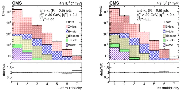
The exclusive jet multiplicity in the selected events is shown in Fig. 1. For both leptonic decay channels, the data show overall agreement with combined signal and background samples from the simulation. The ratio between the cross sections as a function of jet multiplicity in data and in signal plus background simulation, shown in the bottom part of the figure, is compatible with unity within the uncertainties.

6 Unfolding

The distributions of the observables are corrected for event selection efficiencies and for detec-tor resolution effects back to the stable particle level, in order to compare with predictions from event generators simulating Z+jets final states. Particles are considered stable if their proper average lifetime τ satisfies cτ > 10 cm. The correction procedure is based on unfolding tech-niques, as implemented in the ROOUNFOLD toolkit [42], which provides both the “singular value decomposition” (SVD) method [43] and the iterative algorithm based on the Bayes’ the-orem [44]. Both algorithms use a “response matrix” that correlates the values of the observable with and without detector effects.

The response matrix is evaluated using Z+jets events, generated by MADGRAPHfollowed by PYTHIA, with full detector simulation. For generator-level events, leptons and jets are structed from the collection of all stable final-state particles using criteria that mimic the

(8)

recon-6 7 Systematic uncertainties Events 10 2 10 3 10 4 10 5 10 data Z+jets +jets t t diboson +jets τ τ W/Wt (R = 0.5) jets T anti-k | < 2.4 jet η > 30 GeV, | jet T p ee → * γ Z/ (7 TeV) -1 4.9 fb CMS Jet multiplicity 1 2 3 4 5 6 7 data/MC 0 0.5 1 1.5 2 Events 10 2 10 3 10 4 10 5 10 data Z+jets +jets t t diboson +jets τ τ W/Wt (R = 0.5) jets T anti-k | < 2.4 jet η > 30 GeV, | jet T p µ µ → * γ Z/ (7 TeV) -1 4.9 fb CMS Jet multiplicity 1 2 3 4 5 6 7 data/MC 0 0.5 1 1.5 2

Figure 1: Distributions of the exclusive jet multiplicity for the electron channel (left) and muon channel (right). Data are compared to the simulation, which is the sum of signal and back-ground events. Scale factors have been used to correct simulation distributions for residual efficiency differences with respect to data. No unfolding procedure is applied. Only statistical uncertainties are shown.

structed data. Electrons and muons with the highest pT above 20 GeV in the pseudorapidity

range|η| < 2.4 are selected as Z-boson decay products. In order to include the effects of final-state electromagnetic radiation in the generator-level distributions, the electron and muon can-didates are reconstructed by clustering the leptons with all photons in a cone of radius∆R=0.1 in the η–φ plane. Leptons from Z-boson decay are removed from the particle collection used for the jet clustering at generator level. The remaining particles, excluding neutrinos, are clustered into jets using the anti-kT algorithm. A generated jet is included in the analysis if it satisfies

pT > 30 GeV,|η| < 2.4; the jet must contain at least one charged particle, to match the jet re-construction quality requirements used for data analysis, and the distance of the jet from the leptons forming the Z-boson candidate is larger than∆R=0.5.

The unfolded distributions are obtained with the SVD algorithm. As a cross-check, the unfold-ing of the distributions is also performed with the D’Agostini method, which leads to com-patible results within statistical uncertainties. The unfolding has a small effect on the jet η distributions, with migrations among the bins of a few percent for central jets and up to 10% in the outer regions. Larger unfolding effects are observed in the other distributions: up to 20% for the jet multiplicity, between 10% and 20% for the jet pT, and between 10% and 30% for the

HT distribution.

7 Systematic uncertainties

The sources of systematic uncertainties that affect the Z+jets cross section measurement are di-vided into the following categories: jet energy scale (JES) and jet energy resolution (JER) [15], unfolding procedure, efficiency correction and background subtraction, pileup reweighting procedure, and integrated luminosity measurement.

Jet energy scale and resolution uncertainties affect the jet pTreconstruction and the

(9)

7

and pT of the jet. The difference in the distribution of an observable, after varying the JES both

up and down by one standard deviation, is used as an estimate of the JES systematic uncer-tainty. Similarly, the effect of the systematic uncertainties in the scaling factor used in the JER degradation is estimated by varying its value up and down by one standard deviation.

The uncertainty in the unfolding procedure is due to both the statistical uncertainty in the re-sponse matrix from the finite size of the simulated sample and to any dependence on the signal model provided by different event generators. The statistical uncertainty is computed using a MC simulation, which produces variants of the matrix according to random Poisson fluctua-tions of the bin contents. The entire unfolding procedure is repeated for each variant, and the standard deviation of the obtained results is used as an estimate of this uncertainty. The sys-tematic uncertainty due to the generator model is estimated from the difference between events simulated with MADGRAPHandSHERPAat detector response level. The overall unfolding un-certainty is taken to be either the statistical unun-certainty alone, in the case where the results from the two event generators agree within one standard deviation, or the sum in quadrature of the simulation statistical uncertainty and the difference between the two MC generators.

Additional uncertainty arises from the efficiency corrections and from the background sub-traction. The contribution due to efficiency corrections is estimated by adding and subtracting the statistical uncertainties from the tag-and-probe fits. The systematic uncertainty from the background subtraction procedure is small relative to the other sources. For tt and diboson processes, the uncertainty in the normalization arises from both the theoretical uncertainty in the inclusive cross section and the difference between the theoretical prediction of the cross section (as in Section 3) and the corresponding CMS measurement [45–48]. The largest of these two values is taken as the magnitude of the uncertainty. As observed in previous studies [7], the single top quark and W+jets contributions are at the sub-per-mil level, and they are assigned a 100% uncertainty.

Since the background contribution as a function of the jet multiplicity is theoretically less well known than the fully inclusive cross section, control data samples are used to validate the simulation of this dependence. The modeling of the dominant tt background as a function of the jet multiplicity is compared with the data using a control sample enriched in tt events. This sample is selected by requiring the presence of two leptons of different flavors, i.e., eµ combinations, and an agreement is found between data and simulation at the 6% level [7]. The CMS measurement of the tt differential cross section [49], using an event selection compatible with the study presented in this paper, leads to a production rate for events with six jets in simulation overestimated by about 30%. This difference is used as the estimated uncertainty for the six-jets subsample. Variations in the MADGRAPH prediction for tt production from a change in the renormalization, factorization, and matching scales, as well as from the PDF choice, show that data and simulation agree within the estimated uncertainties.

The systematic uncertainty of the pileup reweighting procedure in MC simulation is due to the uncertainties in the minimum-bias cross section and in the instantaneous luminosity of the data sample. This uncertainty is evaluated by varying the number of simulated pileup interactions by±5%. The measurement of the integrated luminosity has an associated uncertainty of 2.2% that directly propagates to any cross section measurement.

The systematic uncertainties (excluding luminosity) used for the combination of the electron and muon samples are summarized in Tables 1, 2, and 3.

(10)

8 8 Results and comparison with theoretical predictions

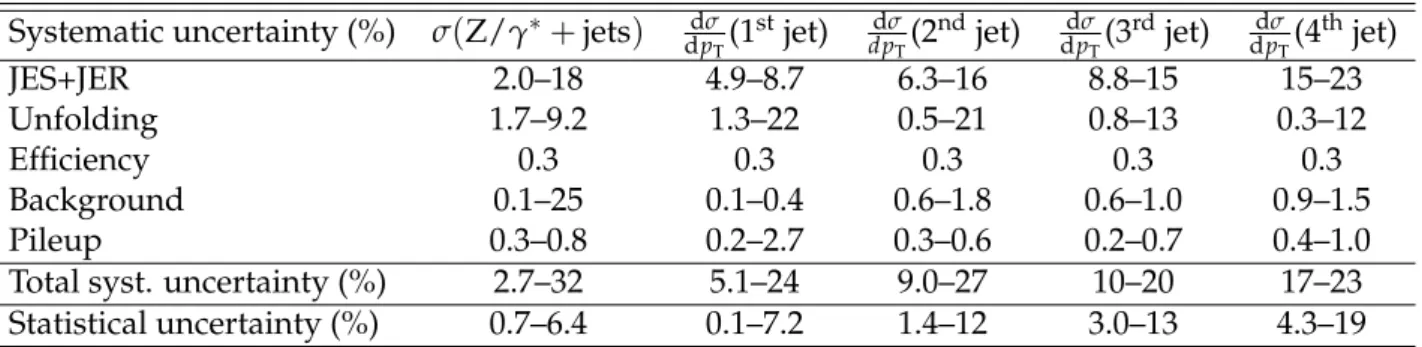
Table 1: Sources of uncertainties (in percent) in the differential exclusive cross section and in the differential cross sections as a function of the jet pT, for each of the four highest pT jets

exclusively. The constant luminosity uncertainty is not included in the total. Systematic uncertainty (%) σ(Z/γ∗+jets) _dpdσ

T(1 st_jet) dσ dpT(2 nd_jet) dσ dpT(3 rd_jet) dσ dpT(4 th_jet) JES+JER 2.0–18 4.9–8.7 6.3–16 8.8–15 15–23 Unfolding 1.7–9.2 1.3–22 0.5–21 0.8–13 0.3–12 Efficiency 0.3 0.3 0.3 0.3 0.3 Background 0.1–25 0.1–0.4 0.6–1.8 0.6–1.0 0.9–1.5 Pileup 0.3–0.8 0.2–2.7 0.3–0.6 0.2–0.7 0.4–1.0

Total syst. uncertainty (%) 2.7–32 5.1–24 9.0–27 10–20 17–23

Statistical uncertainty (%) 0.7–6.4 0.1–7.2 1.4–12 3.0–13 4.3–19

Table 2: Sources of uncertainties (in percent) in the differential cross sections as a function of η, for each of the four highest pT jets exclusively. The constant luminosity uncertainty is not

included in the total.

Systematic uncertainty (%) dσ_dη (1stjet) dσ_dη (2ndjet) dσ_dη (3rdjet) dσ_dη (4thjet)

JES+JER 3.5–8.2 7.2–8.9 9.4–12 13–15

Unfolding 6.5–13 8.4–11 5.0–12 6.4–13

Efficiency 0.3 0.3 0.3 0.3

Background 0.2 0.3–0.5 0.6–1.1 0.9–1.0

Pileup 0.2–0.4 0.3–0.5 0.3–0.7 0.5–1.2

Total syst. uncertainty (%) 7.8–17 11–15 11–19 15–23

Statistical uncertainty (%) 0.6–1.0 0.9–1.4 2.4–3.6 7.6–12

8 Results and comparison with theoretical predictions

The results presented for observable quantities are obtained by combining the unfolded dis-tributions for both leptonic channels into an uncertainty-weighted average for a single lepton flavor. Correlations between systematic uncertainties for the electron and muon channels are taken into account in the combination. Fiducial cross sections are shown, without further cor-rections for the geometrical acceptance or kinematic selection, for leptons and jets. All the results are compared with theoretical distributions, produced with the RIVETtoolkit [50], ob-tained with the generator-level phase space definition and on final-state stable particles as dis-cussed in Section 6. Neutrinos are excluded from the collection of stable particles.

Theoretical predictions at leading order in pQCD are computed with the MADGRAPH 5.1.1 Table 3: Sources of uncertainties (in percent) in the differential cross sections as a function of HT and inclusive jet multiplicity. The constant luminosity uncertainty is not included in the

total. Systematic uncertainty (%) _dHdσ T, Njet ≥1 dσ dHT, Njet ≥2 dσ dHT, Njet ≥3 dσ dHT, Njet ≥4 JES+JER 4.5–9.1 7.0–11 8.6–13 11–17 Unfolding 0.4–17 2.1–18 3.1–22 4.9–23 Efficiency 0.2–0.3 0.3 0.3–0.4 0.3 Background 0.1–0.7 0.3–0.7 0.5–0.8 0.6–1.1 Pileup 0.1–2.3 0.1–2.2 0.3–1.0 0.5–1.0

Total syst. uncertainty (%) 4.6–19 7.8–21 10–26 12–25

(11)

8.1 Jet multiplicity 9

generator followed byPYTHIA6.424 with the Z2 tune and CTEQ6L1 PDF set for fragmentation and parton shower simulation. For the MADGRAPH simulation, the factorization and renor-malization scales are chosen on an event-by-event basis as the transverse mass of the event, clustered with the kT algorithm down to a 2→2 topology, and kT at each vertex splitting,

re-spectively [19, 51]. The MADGRAPHpredictions are rescaled to the available NNLO inclusive cross section [27], which has a uniform associated uncertainty of about 5% that is not propa-gated into the figures.

Predictions at next-to-leading order in QCD are provided bySHERPA2.β2 [22–25, 52], using the CT10 NLO PDF set [53], in a configuration where NLO calculations for Z+0 and Z+1 jet event topologies are merged with leading-order matrix elements for final states with up to four real emissions and matched to the parton shower. The NLO virtual corrections are computed using the BLACKHAT library [54]. In this calculation, the factorization and renormalization scales are defined for each event by clustering the 2→n parton level kinematics onto a core 2→2 configuration using a kT-type algorithm, and using the smallest invariant mass or virtuality in

the core configuration as the scale [52]. The default configuration for the underlying event and fragmentation tune is used.

The third theoretical prediction considered is the NLO QCD calculation for the Z+1 jet ma-trix element as provided by thePOWHEG-BOXpackage [2–4, 55], with CT10 NLO PDF set, and matched with thePYTHIAparton shower evolution using the Z2 tune. In this case, the factor-ization and renormalfactor-ization scales in the inclusive cross section calculation are defined on an event-by-event basis as the Z-boson pT, while for the generation of the radiation they are given

by the pTof the produced radiation.

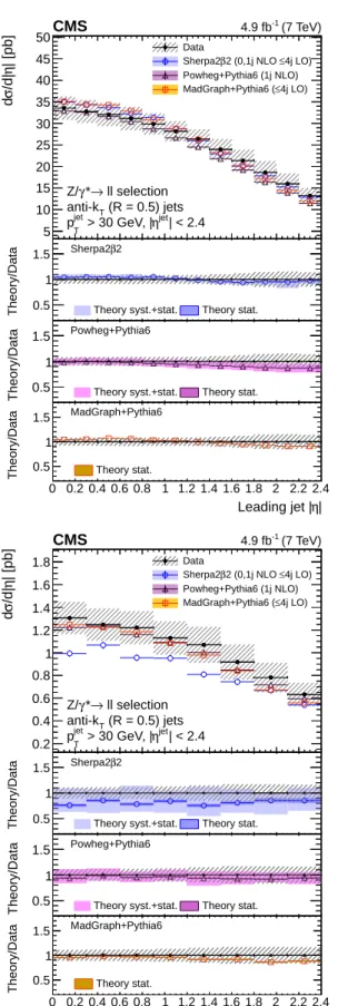
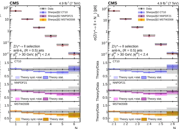
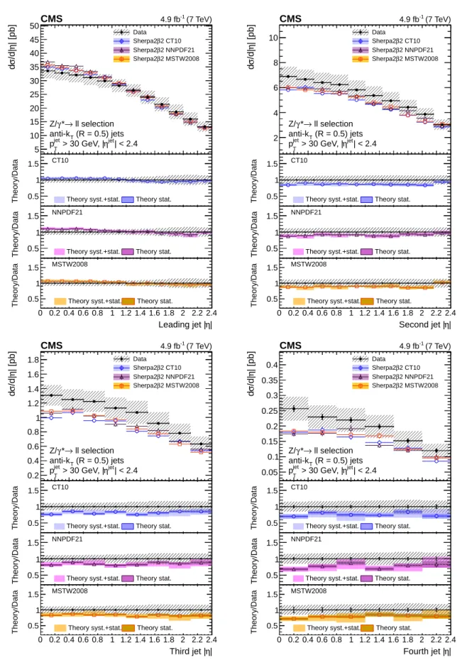
The comparison of these predictions with the corrected data are presented in Figs. 2–5. The effect of PDF choice is shown in Figs. 6–9. The error bars on the plotted data points represent the statistical uncertainty, while cross-hatched bands represent the total experimental uncer-tainty (statistical and systematic uncertainties summed in quadrature) after the unfolding pro-cedure. Uncertainties in the theoretical predictions are shown in the ratio of data to simulation only. For the NLO prediction, theoretical uncertainties are evaluated by varying simultane-ously the factorization and renormalization scales up and down by a factor of two (forSHERPA

andPOWHEG). For theSHERPAprediction only, the resummation scale is changed up and down

by a factor√2 and the parton shower matching scale is changed by 10 GeV in both directions. The effect of the PDF choice is shown for SHERPA, by comparing the results based on CT10 PDF set with those based on the alternative NLO PDFs MSTW2008 and NNPDF2.1 [56]. The theoretical part of the plotted uncertainty band for each PDF choice includes both the intrinsic PDF uncertainty, evaluated according to the prescriptions of the authors of each PDF set, and the effect of the variation of±0.002 in the value of the strong coupling constant αS around the

central value used in the PDF.

8.1 Jet multiplicity

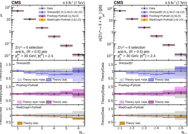
Figure 2 shows the measured cross sections as a function of the exclusive and inclusive jet multiplicities, for a total number of up to six jets in the final state. Beyond the sixth jet, the measurement is not performed due to the statistical limitation of the data and simulated sam-ples. The trend of the jet multiplicity represents the expectation of the pQCD prediction for a staircase-like scaling, with an approximately constant ratio between cross sections for suc-cessive multiplicities [57]. This result confirms the previous observation, which was based on a more statistically limited sample [11]. Within the uncertainties, there is agreement between theory and measurement for both the inclusive and the exclusive distributions.

(12)

10 8 Results and comparison with theoretical predictions 1 2 3 4 5 6 ) [pb] jet ll + N → * γ (Z/ σ -2 10 -1 10 1 10 2 10 ll selection → * γ Z/ (R = 0.5) jets T anti-k | < 2.4 jet η > 30 GeV, | jet T p (7 TeV) -1 4.9 fb CMS Data 4j LO) ≤ 2 (0,1j NLO β Sherpa2 Powheg+Pythia6 (1j NLO) 4j LO) ≤ MadGraph+Pythia6 ( 1 2 3 4 5 6 Theory/Data 0.5 1 1.5 Sherpa2β2

Theory syst.+stat. Theory stat.

1 2 3 4 5 6

Theory/Data 0.5 1

1.5 Powheg+Pythia6

jet N 1 2 3 4 5 6 Theory/Data 0.5 1 1.5 MadGraph+Pythia6 Theory stat. 1 2 3 4 5 6 ) [pb] jet ll + N → * γ (Z/ σ -2 10 -1 10 1 10 2 10 ll selection → * γ Z/ (R = 0.5) jets T anti-k | < 2.4 jet η > 30 GeV, | jet T p (7 TeV) -1 4.9 fb CMS Data 4j LO) ≤ 2 (0,1j NLO β Sherpa2 Powheg+Pythia6 (1j NLO) 4j LO) ≤ MadGraph+Pythia6 ( 1 2 3 4 5 6 Theory/Data 0.5 1 1.5 Sherpa2β2

1 2 3 4 5 6

Theory/Data 0.5 1

1.5 Powheg+Pythia6

jet N 1 ≥ ≥ 2 ≥ 3 ≥ 4 ≥ 5 ≥ 6 Theory/Data 0.5 1 1.5 MadGraph+Pythia6 Theory stat.

Figure 2: Exclusive (left) and inclusive (right) jet multiplicity distributions, after the unfolding procedure, compared withSHERPA,POWHEG, and MADGRAPHpredictions. Error bars around the experimental points represent the statistical uncertainty, while cross-hatched bands repre-sent statistical plus systematic uncertainty. The bands around theory predictions correspond to the statistical uncertainty of the generated sample and, for NLO calculations, to its combination with the systematic uncertainty related to scale variations.

(13)

8.2 Differential cross sections 11

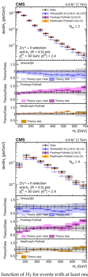
8.2 Differential cross sections

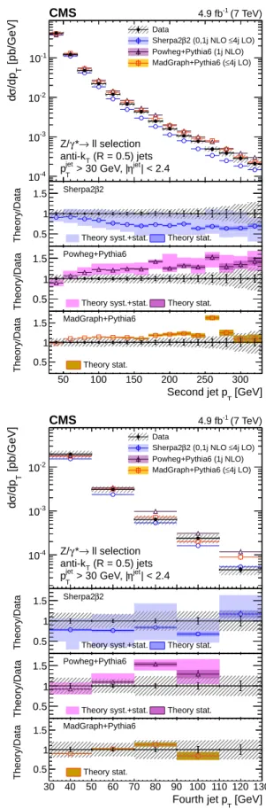
The differential cross sections as a function of jet pT and jet η for the first, second, third, and

fourth highest pT jet in the event are presented in Figs. 3 and 4, respectively. In addition,

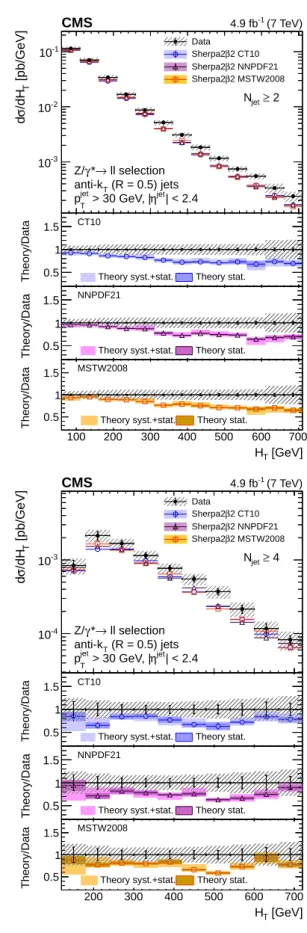
the differential cross sections as a function of HT for events with at least one, two, three, or

four jets are presented in Fig. 5. The pQCD prediction by MADGRAPHprovides a satisfactory description of data for most distributions, but shows an excess in the pT spectra for the first

and second leading jets at pT > 100 GeV. SHERPA tends to underestimate the high pTand HT

regions in most of the spectra, while remaining compatible with the measurement within the estimated theoretical uncertainty. POWHEGpredicts harder pT spectra than those observed in

the data for the events with two or more jets, where the additional hard radiation is described by the parton showers and not by matrix elements. This discrepancy is also reflected in the HT

distribution. Figures 6–9 show no significant dependence of the level of agreement between data and the SHERPAprediction on the PDF set chosen. Hence the PDF choice cannot explain the observed differences with data.

9 Summary

The fiducial production cross section of a Z boson with at least one hadronic jet has been mea-sured in proton-proton collisions at√s = 7 TeV in a sample corresponding to an integrated luminosity of 4.9 fb−1. The measurements comprise inclusive jet multiplicities, exclusive jet multiplicities, and the differential cross sections as a function of jet pT and η for the four

high-est pT jets of the event. In addition, the HT distribution for events with different minimum

numbers of jets has been measured. All measured differential cross sections are corrected for detector effects and compared with theoretical predictions at particle level.

The predictions of calculations combining matrix element and parton shower can describe, within uncertainties, the measured spectra over a wide kinematical range. The measured jet multiplicity distributions and their NLO theoretical predictions from theSHERPAandPOWHEG generators are consistent within the experimental and theoretical uncertainties. However,

SHERPA predicts softer pT and HT spectra than the measured ones, while POWHEGshows an

excess compared to data in the high pTand HTregions. In particular, thePOWHEGspectra are

harder for the highest jet multiplicities, which are described only by parton showers. The tree level calculation based on MADGRAPHpredicts harder pT spectra than the measured ones for

low jet multiplicities.

Acknowledgments

We congratulate our colleagues in the CERN accelerator departments for the excellent perfor-mance of the LHC and thank the technical and administrative staffs at CERN and at other CMS institutes for their contributions to the success of the CMS effort. In addition, we grate-fully acknowledge the computing centres and personnel of the Worldwide LHC Computing Grid for delivering so effectively the computing infrastructure essential to our analyses. Fi-nally, we acknowledge the enduring support for the construction and operation of the LHC and the CMS detector provided by the following funding agencies: the Austrian Federal Min-istry of Science, Research and Economy and the Austrian Science Fund; the Belgian Fonds de la Recherche Scientifique, and Fonds voor Wetenschappelijk Onderzoek; the Brazilian Fund-ing Agencies (CNPq, CAPES, FAPERJ, and FAPESP); the Bulgarian Ministry of Education and Science; CERN; the Chinese Academy of Sciences, Ministry of Science and Technology, and Na-tional Natural Science Foundation of China; the Colombian Funding Agency (COLCIENCIAS);

(14)

12 9 Summary 100 200 300 400 500 600 700 [pb/GeV] T /dp σ d -5 10 -4 10 -3 10 -2 10 -1 10 1 ll selection → * γ Z/ (R = 0.5) jets T anti-k | < 2.4 jet η > 30 GeV, | jet T p (7 TeV) -1 4.9 fb CMS Data 4j LO) ≤ 2 (0,1j NLO β Sherpa2 Powheg+Pythia6 (1j NLO) 4j LO) ≤ MadGraph+Pythia6 ( 100 200 300 400 500 600 700 Theory/Data 0.5 1 1.5 Sherpa2β2

100 200 300 400 500 600 700 Theory/Data 0.5

1

1.5 Powheg+Pythia6

[GeV] T Leading jet p 100 200 300 400 500 600 700 Theory/Data 0.5 1 1.5 MadGraph+Pythia6 Theory stat. 50 100 150 200 250 300 [pb/GeV] T /dp σ d -4 10 -3 10 -2 10 -1 10 ll selection → * γ Z/ (R = 0.5) jets T anti-k | < 2.4 jet η > 30 GeV, | jet T p (7 TeV) -1 4.9 fb CMS Data 4j LO) ≤ 2 (0,1j NLO β Sherpa2 Powheg+Pythia6 (1j NLO) 4j LO) ≤ MadGraph+Pythia6 ( 50 100 150 200 250 300 Theory/Data 0.5 1 1.5 Sherpa2β2

50 100 150 200 250 300 Theory/Data 0.5

1

1.5 Powheg+Pythia6

[GeV] T Second jet p 50 100 150 200 250 300 Theory/Data 0.5 1 1.5 MadGraph+Pythia6 Theory stat. 40 60 80 100 120 140 160 180 [pb/GeV] _T /dp σ d -4 10 -3 10 -2 10 -1 10 ll selection → * γ Z/ (R = 0.5) jets T anti-k | < 2.4 jet η > 30 GeV, | jet T p (7 TeV) -1 4.9 fb CMS Data 4j LO) ≤ 2 (0,1j NLO β Sherpa2 Powheg+Pythia6 (1j NLO) 4j LO) ≤ MadGraph+Pythia6 ( 40 60 80 100 120 140 160 180 Theory/Data 0.5 1 1.5 Sherpa2β2

40 60 80 100 120 140 160 180 Theory/Data 0.5

1

1.5 Powheg+Pythia6

[GeV] T Third jet p 40 60 80 100 120 140 160 180 Theory/Data 0.5 1 1.5 MadGraph+Pythia6 Theory stat. 30 40 50 60 70 80 90 100 110 120 130 [pb/GeV] _T /dp σ d -4 10 -3 10 -2 10 ll selection → * γ Z/ (R = 0.5) jets T anti-k | < 2.4 jet η > 30 GeV, | jet T p (7 TeV) -1 4.9 fb CMS Data 4j LO) ≤ 2 (0,1j NLO β Sherpa2 Powheg+Pythia6 (1j NLO) 4j LO) ≤ MadGraph+Pythia6 ( 30 40 50 60 70 80 90 100 110 120 130 Theory/Data 0.5 1 1.5 Sherpa2β2

30 40 50 60 70 80 90 100 110 120 130 Theory/Data 0.5

1

1.5 Powheg+Pythia6

[GeV] T Fourth jet p 30 40 50 60 70 80 90 100 110 120 130 Theory/Data 0.5 1 1.5 MadGraph+Pythia6 Theory stat.

Figure 3: Unfolded differential cross section as a function of pTfor the first (top left), second (top

right), third (bottom left), and fourth (bottom right) highest pT jets, compared with SHERPA,

POWHEG, and MADGRAPH predictions. Error bars around the experimental points represent

the statistical uncertainty, while cross-hatched bands represent statistical plus systematic un-certainty. The bands around theory predictions correspond to the statistical uncertainty of the generated sample and, for NLO calculations, to its combination with systematic uncertainty related to scale variations.

(15)

13 0 0.2 0.4 0.6 0.8 1 1.2 1.4 1.6 1.8 2 2.2 2.4 | [pb] η /d| σ d 5 10 15 20 25 30 35 40 45 50 ll selection → * γ Z/ (R = 0.5) jets T anti-k | < 2.4 jet η > 30 GeV, | jet T p (7 TeV) -1 4.9 fb CMS Data 4j LO) ≤ 2 (0,1j NLO β Sherpa2 Powheg+Pythia6 (1j NLO) 4j LO) ≤ MadGraph+Pythia6 ( 0 0.2 0.4 0.6 0.8 1 1.2 1.4 1.6 1.8 2 2.2 2.4 Theory/Data 0.5 1 1.5 Sherpa2β2

0 0.2 0.4 0.6 0.8 1 1.2 1.4 1.6 1.8 2 2.2 2.4 Theory/Data 0.5

1

1.5 Powheg+Pythia6

| η Leading jet | 0 0.2 0.4 0.6 0.8 1 1.2 1.4 1.6 1.8 2 2.2 2.4 Theory/Data 0.5 1 1.5 MadGraph+Pythia6 Theory stat. 0 0.2 0.4 0.6 0.8 1 1.2 1.4 1.6 1.8 2 2.2 2.4 | [pb] η /d| σ d 2 4 6 8 10 ll selection → * γ Z/ (R = 0.5) jets T anti-k | < 2.4 jet η > 30 GeV, | jet T p (7 TeV) -1 4.9 fb CMS Data 4j LO) ≤ 2 (0,1j NLO β Sherpa2 Powheg+Pythia6 (1j NLO) 4j LO) ≤ MadGraph+Pythia6 ( 0 0.2 0.4 0.6 0.8 1 1.2 1.4 1.6 1.8 2 2.2 2.4 Theory/Data 0.5 1 1.5 Sherpa2β2

0 0.2 0.4 0.6 0.8 1 1.2 1.4 1.6 1.8 2 2.2 2.4 Theory/Data 0.5

1

1.5 Powheg+Pythia6

| η Second jet | 0 0.2 0.4 0.6 0.8 1 1.2 1.4 1.6 1.8 2 2.2 2.4 Theory/Data 0.5 1 1.5 MadGraph+Pythia6 Theory stat. 0 0.2 0.4 0.6 0.8 1 1.2 1.4 1.6 1.8 2 2.2 2.4 | [pb] η /d| σ d 0.2 0.4 0.6 0.8 1 1.2 1.4 1.6 1.8 ll selection → * γ Z/ (R = 0.5) jets T anti-k | < 2.4 jet η > 30 GeV, | jet T p (7 TeV) -1 4.9 fb CMS Data 4j LO) ≤ 2 (0,1j NLO β Sherpa2 Powheg+Pythia6 (1j NLO) 4j LO) ≤ MadGraph+Pythia6 ( 0 0.2 0.4 0.6 0.8 1 1.2 1.4 1.6 1.8 2 2.2 2.4 Theory/Data 0.5 1 1.5 Sherpa2β2

0 0.2 0.4 0.6 0.8 1 1.2 1.4 1.6 1.8 2 2.2 2.4 Theory/Data 0.5

1

1.5 Powheg+Pythia6

| η Third jet | 0 0.2 0.4 0.6 0.8 1 1.2 1.4 1.6 1.8 2 2.2 2.4 Theory/Data 0.5 1 1.5 MadGraph+Pythia6 Theory stat. 0 0.2 0.4 0.6 0.8 1 1.2 1.4 1.6 1.8 2 2.2 2.4 | [pb] η /d| σ d 0.05 0.1 0.15 0.2 0.25 0.3 0.35 0.4 ll selection → * γ Z/ (R = 0.5) jets T anti-k | < 2.4 jet η > 30 GeV, | jet T p (7 TeV) -1 4.9 fb CMS Data 4j LO) ≤ 2 (0,1j NLO β Sherpa2 Powheg+Pythia6 (1j NLO) 4j LO) ≤ MadGraph+Pythia6 ( 0 0.2 0.4 0.6 0.8 1 1.2 1.4 1.6 1.8 2 2.2 2.4 Theory/Data 0.5 1 1.5 Sherpa2β2

0 0.2 0.4 0.6 0.8 1 1.2 1.4 1.6 1.8 2 2.2 2.4 Theory/Data 0.5

1

1.5 Powheg+Pythia6

| η Fourth jet | 0 0.2 0.4 0.6 0.8 1 1.2 1.4 1.6 1.8 2 2.2 2.4 Theory/Data 0.5 1 1.5 MadGraph+Pythia6 Theory stat.

Figure 4: Unfolded differential cross section as a function of the jet absolute pseudorapidity|η| for the first (top left), second (top right), third (bottom left), and fourth (bottom right) highest pT jets, compared withSHERPA,POWHEG, and MADGRAPHpredictions. Error bars around the

experimental points represent the statistical uncertainty, while cross-hatched bands represent statistical plus systematic uncertainty. The bands around theory predictions correspond to the statistical uncertainty of the generated sample and, for NLO calculations, to its combination with systematic uncertainty related to scale variations.

(16)

14 9 Summary 100 200 300 400 500 600 700 [pb/GeV] T /dH σ d -3 10 -2 10 -1 10 1 ll selection → * γ Z/ (R = 0.5) jets T anti-k | < 2.4 jet η > 30 GeV, | jet T p (7 TeV) -1 4.9 fb CMS 1 ≥ jet N Data 4j LO) ≤ 2 (0,1j NLO β Sherpa2 Powheg+Pythia6 (1j NLO) 4j LO) ≤ MadGraph+Pythia6 ( 100 200 300 400 500 600 700 Theory/Data 0.5 1 1.5 Sherpa2β2

100 200 300 400 500 600 700 Theory/Data 0.5

1

1.5 Powheg+Pythia6

[GeV] T H 100 200 300 400 500 600 700 Theory/Data 0.5 1 1.5 MadGraph+Pythia6 Theory stat. 100 200 300 400 500 600 700 [pb/GeV] T /dH σ d -3 10 -2 10 -1 10 ll selection → * γ Z/ (R = 0.5) jets T anti-k | < 2.4 jet η > 30 GeV, | jet T p (7 TeV) -1 4.9 fb CMS 2 ≥ jet N Data 4j LO) ≤ 2 (0,1j NLO β Sherpa2 Powheg+Pythia6 (1j NLO) 4j LO) ≤ MadGraph+Pythia6 ( 100 200 300 400 500 600 700 Theory/Data 0.5 1 1.5 Sherpa2β2

100 200 300 400 500 600 700 Theory/Data 0.5

1

1.5 Powheg+Pythia6

[GeV] T H 100 200 300 400 500 600 700 Theory/Data 0.5 1 1.5 MadGraph+Pythia6 Theory stat. 100 200 300 400 500 600 700 [pb/GeV]_T /dH σ d -4 10 -3 10 -2 10 ll selection → * γ Z/ (R = 0.5) jets T anti-k | < 2.4 jet η > 30 GeV, | jet T p (7 TeV) -1 4.9 fb CMS 3 ≥ jet N Data 4j LO) ≤ 2 (0,1j NLO β Sherpa2 Powheg+Pythia6 (1j NLO) 4j LO) ≤ MadGraph+Pythia6 ( 100 200 300 400 500 600 700 Theory/Data 0.5 1 1.5 Sherpa2β2

100 200 300 400 500 600 700 Theory/Data 0.5

1

1.5 Powheg+Pythia6

[GeV] T H 100 200 300 400 500 600 700 Theory/Data 0.5 1 1.5 MadGraph+Pythia6 Theory stat. 200 300 400 500 600 700 [pb/GeV]_T /dH σ d -4 10 -3 10 ll selection → * γ Z/ (R = 0.5) jets T anti-k | < 2.4 jet η > 30 GeV, | jet T p (7 TeV) -1 4.9 fb CMS 4 ≥ jet N Data 4j LO) ≤ 2 (0,1j NLO β Sherpa2 Powheg+Pythia6 (1j NLO) 4j LO) ≤ MadGraph+Pythia6 ( 200 300 400 500 600 700 Theory/Data 0.5 1 1.5 Sherpa2β2

200 300 400 500 600 700 Theory/Data 0.5

1

1.5 Powheg+Pythia6

[GeV] T H 200 300 400 500 600 700 Theory/Data 0.5 1 1.5 MadGraph+Pythia6 Theory stat.

Figure 5: Unfolded differential cross section as a function of HTfor events with at least one (top

left), two (top right), three (bottom left), and four (bottom right) jets compared withSHERPA,

POWHEG, and MADGRAPH predictions. Error bars around the experimental points represent

the statistical uncertainty, while cross-hatched bands represent statistical plus systematic un-certainty. The bands around theory predictions correspond to the statistical uncertainty of the generated sample and, for NLO calculations, to its combination with systematic uncertainty related to scale variations.

(17)

15 1 2 3 4 5 6 ) [pb] jet ll + N → * γ (Z/ σ -2 10 -1 10 1 10 2 10 ll selection → * γ Z/ (R = 0.5) jets T anti-k | < 2.4 jet η > 30 GeV, | jet T p (7 TeV) -1 4.9 fb CMS Data 2 CT10 β Sherpa2 2 NNPDF21 β Sherpa2 2 MSTW2008 β Sherpa2 1 2 3 4 5 6 Theory/Data 0.5 1 1.5 CT10

1 2 3 4 5 6

Theory/Data 0.5 1

1.5 NNPDF21

jet N 1 2 3 4 5 6 Theory/Data 0.5 1 1.5 MSTW2008

1 2 3 4 5 6 ) [pb] jet ll + N → * γ (Z/ σ -2 10 -1 10 1 10 2 10 ll selection → * γ Z/ (R = 0.5) jets T anti-k | < 2.4 jet η > 30 GeV, | jet T p (7 TeV) -1 4.9 fb CMS Data 2 CT10 β Sherpa2 2 NNPDF21 β Sherpa2 2 MSTW2008 β Sherpa2 1 2 3 4 5 6 Theory/Data 0.5 1 1.5 CT10

1 2 3 4 5 6

Theory/Data 0.5 1

1.5 NNPDF21

jet N 1 ≥ ≥ 2 ≥ 3 ≥ 4 ≥ 5 ≥ 6 Theory/Data 0.5 1 1.5 MSTW2008

Figure 6: Exclusive jet multiplicity distribution (left) and inclusive jet multiplicity distribu-tion (right), after the unfolding procedure, compared with SHERPA predictions based on the PDF sets CT10, MSTW2008, and NNPDF2.1. Error bars around the experimental points repre-sent the statistical uncertainty, while cross-hatched bands reprerepre-sent statistical plus systematic uncertainty. The bands around theory predictions correspond to the statistical uncertainty of the generated sample and to its combination with the theoretical PDF uncertainty.

(18)

16 9 Summary 100 200 300 400 500 600 700 [pb/GeV] T /dp σ d -5 10 -4 10 -3 10 -2 10 -1 10 1 ll selection → * γ Z/ (R = 0.5) jets T anti-k | < 2.4 jet η > 30 GeV, | jet T p (7 TeV) -1 4.9 fb CMS Data 2 CT10 β Sherpa2 2 NNPDF21 β Sherpa2 2 MSTW2008 β Sherpa2 100 200 300 400 500 600 700 Theory/Data 0.5 1 1.5 CT10

100 200 300 400 500 600 700 Theory/Data 0.5

1

1.5 NNPDF21

[GeV] T Leading jet p 100 200 300 400 500 600 700 Theory/Data 0.5 1 1.5 MSTW2008

50 100 150 200 250 300 [pb/GeV] T /dp σ d -4 10 -3 10 -2 10 -1 10 ll selection → * γ Z/ (R = 0.5) jets T anti-k | < 2.4 jet η > 30 GeV, | jet T p (7 TeV) -1 4.9 fb CMS Data 2 CT10 β Sherpa2 2 NNPDF21 β Sherpa2 2 MSTW2008 β Sherpa2 50 100 150 200 250 300 Theory/Data 0.5 1 1.5 CT10

50 100 150 200 250 300 Theory/Data 0.5

1

1.5 NNPDF21

[GeV] T Second jet p 50 100 150 200 250 300 Theory/Data 0.5 1 1.5 MSTW2008

40 60 80 100 120 140 160 180 [pb/GeV] _T /dp σ d -4 10 -3 10 -2 10 -1 10 ll selection → * γ Z/ (R = 0.5) jets T anti-k | < 2.4 jet η > 30 GeV, | jet T p (7 TeV) -1 4.9 fb CMS Data 2 CT10 β Sherpa2 2 NNPDF21 β Sherpa2 2 MSTW2008 β Sherpa2 40 60 80 100 120 140 160 180 Theory/Data 0.5 1 1.5 CT10

40 60 80 100 120 140 160 180 Theory/Data 0.5

1

1.5 NNPDF21

[GeV] T Third jet p 40 60 80 100 120 140 160 180 Theory/Data 0.5 1 1.5 MSTW2008

30 40 50 60 70 80 90 100 110 120 130 [pb/GeV] _T /dp σ d -4 10 -3 10 -2 10 ll selection → * γ Z/ (R = 0.5) jets T anti-k | < 2.4 jet η > 30 GeV, | jet T p (7 TeV) -1 4.9 fb CMS Data 2 CT10 β Sherpa2 2 NNPDF21 β Sherpa2 2 MSTW2008 β Sherpa2 30 40 50 60 70 80 90 100 110 120 130 Theory/Data 0.5 1 1.5 CT10

30 40 50 60 70 80 90 100 110 120 130 Theory/Data 0.5

1

1.5 NNPDF21

[GeV] T Fourth jet p 30 40 50 60 70 80 90 100 110 120 130 Theory/Data 0.5 1 1.5 MSTW2008

Figure 7: Unfolded differential cross section as a function of pT for the first (top left), second

(top right), third (bottom left), and fourth (bottom right) highest pTjets, compared withSHERPA

predictions based on the PDF sets CT10, MSTW2008, and NNPDF2.1. Error bars around the experimental points represent the statistical uncertainty, while cross-hatched bands represent statistical plus systematic uncertainty. The bands around theory predictions correspond to the statistical uncertainty of the generated sample and to its combination with the theoretical PDF uncertainty.

(19)

17 0 0.2 0.4 0.6 0.8 1 1.2 1.4 1.6 1.8 2 2.2 2.4 | [pb] η /d| σ d 5 10 15 20 25 30 35 40 45 50 ll selection → * γ Z/ (R = 0.5) jets T anti-k | < 2.4 jet η > 30 GeV, | jet T p (7 TeV) -1 4.9 fb CMS Data 2 CT10 β Sherpa2 2 NNPDF21 β Sherpa2 2 MSTW2008 β Sherpa2 0 0.2 0.4 0.6 0.8 1 1.2 1.4 1.6 1.8 2 2.2 2.4 Theory/Data 0.5 1 1.5 CT10

0 0.2 0.4 0.6 0.8 1 1.2 1.4 1.6 1.8 2 2.2 2.4 Theory/Data 0.5

1

1.5 NNPDF21

| η Leading jet | 0 0.2 0.4 0.6 0.8 1 1.2 1.4 1.6 1.8 2 2.2 2.4 Theory/Data 0.5 1 1.5 MSTW2008

0 0.2 0.4 0.6 0.8 1 1.2 1.4 1.6 1.8 2 2.2 2.4 | [pb] η /d| σ d 2 4 6 8 10 ll selection → * γ Z/ (R = 0.5) jets T anti-k | < 2.4 jet η > 30 GeV, | jet T p (7 TeV) -1 4.9 fb CMS Data 2 CT10 β Sherpa2 2 NNPDF21 β Sherpa2 2 MSTW2008 β Sherpa2 0 0.2 0.4 0.6 0.8 1 1.2 1.4 1.6 1.8 2 2.2 2.4 Theory/Data 0.5 1 1.5 CT10

0 0.2 0.4 0.6 0.8 1 1.2 1.4 1.6 1.8 2 2.2 2.4 Theory/Data 0.5

1

1.5 NNPDF21

| η Second jet | 0 0.2 0.4 0.6 0.8 1 1.2 1.4 1.6 1.8 2 2.2 2.4 Theory/Data 0.5 1 1.5 MSTW2008

0 0.2 0.4 0.6 0.8 1 1.2 1.4 1.6 1.8 2 2.2 2.4 | [pb] η /d| σ d 0.2 0.4 0.6 0.8 1 1.2 1.4 1.6 1.8 ll selection → * γ Z/ (R = 0.5) jets T anti-k | < 2.4 jet η > 30 GeV, | jet T p (7 TeV) -1 4.9 fb CMS Data 2 CT10 β Sherpa2 2 NNPDF21 β Sherpa2 2 MSTW2008 β Sherpa2 0 0.2 0.4 0.6 0.8 1 1.2 1.4 1.6 1.8 2 2.2 2.4 Theory/Data 0.5 1 1.5 CT10

0 0.2 0.4 0.6 0.8 1 1.2 1.4 1.6 1.8 2 2.2 2.4 Theory/Data 0.5

1

1.5 NNPDF21

| η Third jet | 0 0.2 0.4 0.6 0.8 1 1.2 1.4 1.6 1.8 2 2.2 2.4 Theory/Data 0.5 1 1.5 MSTW2008

0 0.2 0.4 0.6 0.8 1 1.2 1.4 1.6 1.8 2 2.2 2.4 | [pb] η /d| σ d 0.05 0.1 0.15 0.2 0.25 0.3 0.35 0.4 ll selection → * γ Z/ (R = 0.5) jets T anti-k | < 2.4 jet η > 30 GeV, | jet T p (7 TeV) -1 4.9 fb CMS Data 2 CT10 β Sherpa2 2 NNPDF21 β Sherpa2 2 MSTW2008 β Sherpa2 0 0.2 0.4 0.6 0.8 1 1.2 1.4 1.6 1.8 2 2.2 2.4 Theory/Data 0.5 1 1.5 CT10

0 0.2 0.4 0.6 0.8 1 1.2 1.4 1.6 1.8 2 2.2 2.4 Theory/Data 0.5

1

1.5 NNPDF21

| η Fourth jet | 0 0.2 0.4 0.6 0.8 1 1.2 1.4 1.6 1.8 2 2.2 2.4 Theory/Data 0.5 1 1.5 MSTW2008

Figure 8: Unfolded differential cross section as a function of the jet absolute pseudorapidity |η|for the first (top left), second (top right), third (bottom left), and fourth (bottom right) high-est pT jets, compared with SHERPA predictions based on the PDF sets CT10, MSTW2008, and

NNPDF2.1. Error bars around the experimental points represent the statistical uncertainty, while cross-hatched bands represent statistical plus systematic uncertainty. The bands around theory predictions correspond to the statistical uncertainty of the generated sample and to its combination with the theoretical PDF uncertainty.

(20)

18 9 Summary 100 200 300 400 500 600 700 [pb/GeV] T /dH σ d -3 10 -2 10 -1 10 1 ll selection → * γ Z/ (R = 0.5) jets T anti-k | < 2.4 jet η > 30 GeV, | jet T p (7 TeV) -1 4.9 fb CMS 1 ≥ jet N Data 2 CT10 β Sherpa2 2 NNPDF21 β Sherpa2 2 MSTW2008 β Sherpa2 100 200 300 400 500 600 700 Theory/Data 0.5 1 1.5 CT10

100 200 300 400 500 600 700 Theory/Data 0.5

1

1.5 NNPDF21

[GeV] T H 100 200 300 400 500 600 700 Theory/Data 0.5 1 1.5 MSTW2008

100 200 300 400 500 600 700 [pb/GeV] T /dH σ d -3 10 -2 10 -1 10 ll selection → * γ Z/ (R = 0.5) jets T anti-k | < 2.4 jet η > 30 GeV, | jet T p (7 TeV) -1 4.9 fb CMS 2 ≥ jet N Data 2 CT10 β Sherpa2 2 NNPDF21 β Sherpa2 2 MSTW2008 β Sherpa2 100 200 300 400 500 600 700 Theory/Data 0.5 1 1.5 CT10

100 200 300 400 500 600 700 Theory/Data 0.5

1

1.5 NNPDF21

100 200 300 400 500 600 700 [pb/GeV]_T /dH σ d -4 10 -3 10 -2 10 ll selection → * γ Z/ (R = 0.5) jets T anti-k | < 2.4 jet η > 30 GeV, | jet T p (7 TeV) -1 4.9 fb CMS 3 ≥ jet N Data 2 CT10 β Sherpa2 2 NNPDF21 β Sherpa2 2 MSTW2008 β Sherpa2 100 200 300 400 500 600 700 Theory/Data 0.5 1 1.5 CT10

100 200 300 400 500 600 700 Theory/Data 0.5

1

1.5 NNPDF21

200 300 400 500 600 700 [pb/GeV]_T /dH σ d -4 10 -3 10 ll selection → * γ Z/ (R = 0.5) jets T anti-k | < 2.4 jet η > 30 GeV, | jet T p (7 TeV) -1 4.9 fb CMS 4 ≥ jet N Data 2 CT10 β Sherpa2 2 NNPDF21 β Sherpa2 2 MSTW2008 β Sherpa2 200 300 400 500 600 700 Theory/Data 0.5 1 1.5 CT10

200 300 400 500 600 700 Theory/Data 0.5

1

1.5 NNPDF21

[GeV] T H 200 300 400 500 600 700 Theory/Data 0.5 1 1.5 MSTW2008

Figure 9: Unfolded differential cross section as a function of HTfor events with at least one (top

left), two (top right), three (bottom left), and four (bottom right) jets compared withSHERPA predictions based on the PDF sets CT10, MSTW2008, and NNPDF2.1. Error bars around the experimental points represent the statistical uncertainty, while cross-hatched bands represent statistical plus systematic uncertainty. The bands around theory predictions correspond to the statistical uncertainty of the generated sample and to its combination with the theoretical PDF uncertainty.

(21)

References 19

the Croatian Ministry of Science, Education and Sport, and the Croatian Science Foundation; the Research Promotion Foundation, Cyprus; the Ministry of Education and Research, Esto-nian Research Council via IUT23-4 and IUT23-6 and European Regional Development Fund, Estonia; the Academy of Finland, Finnish Ministry of Education and Culture, and Helsinki Institute of Physics; the Institut National de Physique Nucléaire et de Physique des Partic-ules / CNRS, and Commissariat à l’ Énergie Atomique et aux Énergies Alternatives / CEA, France; the Bundesministerium f ür Bildung und Forschung, Deutsche Forschungsgemeinschaft, and Helmholtz-Gemeinschaft Deutscher Forschungszentren, Germany; the General Secretariat for Research and Technology, Greece; the National Scientific Research Foundation, and Na-tional Innovation Office, Hungary; the Department of Atomic Energy and the Department of Science and Technology, India; the Institute for Studies in Theoretical Physics and Mathematics, Iran; the Science Foundation, Ireland; the Istituto Nazionale di Fisica Nucleare, Italy; the Ko-rean Ministry of Education, Science and Technology and the World Class University program of NRF, Republic of Korea; the Lithuanian Academy of Sciences; the Ministry of Education, and University of Malaya (Malaysia); the Mexican Funding Agencies (CINVESTAV, CONACYT, SEP, and UASLP-FAI); the Ministry of Business, Innovation and Employment, New Zealand; the Pakistan Atomic Energy Commission; the Ministry of Science and Higher Education and the National Science Centre, Poland; the Fundação para a Ciência e a Tecnologia, Portugal; JINR, Dubna; the Ministry of Education and Science of the Russian Federation, the Federal Agency of Atomic Energy of the Russian Federation, Russian Academy of Sciences, and the Russian Foundation for Basic Research; the Ministry of Education, Science and Technologi-cal Development of Serbia; the Secretar´ıa de Estado de Investigaci ón, Desarrollo e Innovaci ón and Programa Consolider-Ingenio 2010, Spain; the Swiss Funding Agencies (ETH Board, ETH Zurich, PSI, SNF, UniZH, Canton Zurich, and SER); the Ministry of Science and Technology, Taipei; the Thailand Center of Excellence in Physics, the Institute for the Promotion of Teach-ing Science and Technology of Thailand, Special Task Force for ActivatTeach-ing Research and the National Science and Technology Development Agency of Thailand; the Scientific and Techni-cal Research Council of Turkey, and Turkish Atomic Energy Authority; the National Academy of Sciences of Ukraine, and State Fund for Fundamental Researches, Ukraine; the Science and Technology Facilities Council, UK; the US Department of Energy, and the US National Science Foundation.

Individuals have received support from the Marie-Curie programme and the European Re-search Council and EPLANET (European Union); the Leventis Foundation; the A. P. Sloan Foundation; the Alexander von Humboldt Foundation; the Belgian Federal Science Policy Of-fice; the Fonds pour la Formation `a la Recherche dans l’Industrie et dans l’Agriculture (FRIA-Belgium); the Agentschap voor Innovatie door Wetenschap en Technologie (IWT-(FRIA-Belgium); the Ministry of Education, Youth and Sports (MEYS) of the Czech Republic; the Council of Sci-ence and Industrial Research, India; the HOMING PLUS programme of Foundation for Polish Science, cofinanced from European Union, Regional Development Fund; the Compagnia di San Paolo (Torino); the Consorzio per la Fisica (Trieste); MIUR project 20108T4XTM (Italy); the Thalis and Aristeia programmes cofinanced by EU-ESF and the Greek NSRF; and the National Priorities Research Program by Qatar National Research Fund.

References

[1] J. Alwall et al., “MadGraph 5: going beyond”, JHEP 06 (2011) 128,

doi:10.1007/JHEP06(2011)128, arXiv:1106.0522.

(22)

20 References

algorithms”, JHEP 11 (2004) 040, doi:10.1088/1126-6708/2004/11/040, arXiv:hep-ph/0409146.

[3] S. Frixione, P. Nason, and C. Oleari, “Matching NLO QCD computations with parton shower simulations: the POWHEG method”, JHEP 11 (2007) 070,

doi:10.1088/1126-6708/2007/11/070, arXiv:0709.2092.

[4] S. Alioli, P. Nason, C. Oleari, and E. Re, “A general framework for implementing NLO calculations in shower Monte Carlo programs: the POWHEG BOX”, JHEP 06 (2010) 043,

doi:10.1007/JHEP06(2010)043, arXiv:1002.2581.

[5] CMS Collaboration, “Search for the standard model Higgs boson produced in association with a W or a Z boson and decaying to bottom quarks”, Phys. Rev. D 89 (2014) 012003,

doi:10.1103/PhysRevD.89.012003, arXiv:1310.3687.

[6] ATLAS Collaboration, “Search for the bb decay of the Standard Model Higgs boson in associated (W/Z)H production with the ATLAS detector”, JHEP 01 (2015) 069, doi:10.1007/JHEP01(2015)069, arXiv:1409.6212.

[7] CMS Collaboration, “Event shapes and azimuthal correlations in Z + jets events in pp collisions at√s=7 TeV”, Phys. Lett. B 722 (2013) 238,

doi:10.1016/j.physletb.2013.04.025, arXiv:1301.1646.

[8] CDF Collaboration, “Measurement of inclusive jet cross-sections in Z/γ∗(→e+e−) + jets production in p ¯p collisions at√s = 1.96 TeV”, Phys. Rev. Lett. 100 (2008) 102001,

doi:10.1103/PhysRevLett.100.102001, arXiv:0711.3717.

[9] D0 Collaboration, “Measurements of differential cross sections of Z/γ∗+jets+X events in p ¯p collisions at√s = 1.96 TeV”, Phys. Lett. B 678 (2009) 45,

doi:10.1016/j.physletb.2009.05.058, arXiv:0903.1748.

[10] ATLAS Collaboration, “Measurement of the production cross section for Z/γ∗in

association with jets in pp collisions at√s = 7 TeV with the ATLAS detector”, Phys. Rev. D 85 (2012) 032009, doi:10.1103/PhysRevD.85.032009, arXiv:1111.2690. [11] CMS Collaboration, “Jet production rates in association with W and Z bosons in pp

collisions at√s = 7 TeV”, JHEP 01 (2012) 010, doi:10.1007/JHEP01(2012)010, arXiv:1110.3226.

[12] ATLAS Collaboration, “Measurement of the production cross section of jets in association with a Z boson in pp collisions at√s = 7 TeV with the ATLAS detector”, JHEP 07 (2013) 032, doi:10.1007/JHEP07(2013)032, arXiv:1304.7098.

[13] CMS Collaboration, “Absolute Calibration of the Luminosity Measurement at CMS: Winter 2012 Update”, CMS Physics Analysis Summary CMS-PAS-SMP-12-008, 2012. [14] CMS Collaboration, “The CMS experiment at the CERN LHC”, JINST 3 (2008) S08004,

doi:10.1088/1748-0221/3/08/S08004.

[15] CMS Collaboration, “Determination of jet energy calibration and transverse momentum resolution in CMS”, JINST 6 (2011) P11002,

(23)

References 21

[16] P. Jonathan et al., “New generation of parton distributions with uncertainties from global QCD analysis”, JHEP 07 (2002) 012, doi:10.1088/1126-6708/2002/07/012, arXiv:hep-ph/0201195.

[17] T. Sj ¨ostrand, S. Mrenna, and P. Skands, “PYTHIA 6.4 physics and manual”, JHEP 05 (2006) 026, doi:10.1088/1126-6708/2006/05/026, arXiv:hep-ph/0603175. [18] CMS Collaboration, “Charged particle multiplicities in pp interactions at√s = 0.9, 2.36,

and 7 TeV”, JHEP 01 (2011) 079, doi:10.1007/JHEP01(2011)079, arXiv:1011.5531.

[19] J. Alwall et al., “Comparative study of various algorithms for the merging of parton showers and matrix elements in hadronic collisions”, Eur. Phys. J. C 53 (2008) 473, doi:10.1140/epjc/s10052-007-0490-5, arXiv:0706.2569.

[20] P. Golonka et al., “The tauola-photos-F environment for the TAUOLA and PHOTOS packages, release II”, Comput. Phys. Commun. 174 (2006) 818,

doi:10.1016/j.cpc.2005.12.018, arXiv:hep-ph/0312240.

[21] E. Re, “Single-top W t-channel production matched with parton showers using the POWHEG method”, Eur. Phys. J. C 71 (2011) 1547,

doi:10.1140/epjc/s10052-011-1547-z, arXiv:1009.2450.

[22] T. Gleisberg and S. H ¨oche, “Comix, a new matrix element generator”, JHEP 12 (2008) 039, doi:10.1088/1126-6708/2008/12/039, arXiv:0808.3674.

[23] S. Schumann and F. Krauss, “A parton shower algorithm based on Catani-Seymour dipole factorisation”, JHEP 03 (2008) 038, doi:10.1088/1126-6708/2008/03/038,

arXiv:0709.1027.

[24] T. Gleisberg et al., “Event generation with SHERPA 1.1”, JHEP 02 (2009) 007, doi:10.1088/1126-6708/2009/02/007, arXiv:0811.4622.

[25] S. H ¨oche, F. Krauss, S. Schumann, and F. Siegert, “QCD matrix elements and truncated showers”, JHEP 05 (2009) 053, doi:10.1088/1126-6708/2009/05/053,

arXiv:0903.1219.

[26] P. M. Nadolsky et al., “Implications of CTEQ global analysis for collider observables”, Phys. Rev. D 78 (2008) 013004, doi:10.1103/PhysRevD.78.013004,

arXiv:0802.0007.

[27] K. Melnikov and F. Petriello, “Electroweak gauge boson production at hadron colliders through O(α2_s)”, Phys. Rev. D 74 (2006) 114017, doi:10.1103/PhysRevD.74.114017,

arXiv:hep-ph/0609070.

[28] A. D. Martin, W. J. Stirling, R. S. Thorne, and G. Watt, “Parton distributions for the LHC”, Eur. Phys. J. C 63 (2009) 189, doi:10.1140/epjc/s10052-009-1072-5,

arXiv:0901.0002.

[29] M. Czakon, P. Fiedler, and A. Mitov, “Total Top-Quark Pair-Production Cross Section at Hadron Colliders ThroughO(α4_S)”, Phys. Rev. Lett. 110 (2013) 252004,

doi:10.1103/PhysRevLett.110.252004, arXiv:1303.6254.

[30] J. M. Campbell, R. K. Ellis, and C. Williams, “Vector boson pair production at the LHC”, JHEP 07 (2011) 018, doi:10.1007/JHEP07(2011)018, arXiv:1105.0020.

(24)

22 References

[31] S. Agostinelli et al., “GEANT4—a simulation toolkit”, Nucl. Instrum. Meth. A 506 (2003) 250, doi:10.1016/S0168-9002(03)01368-8.

[32] J. Allison et al., “GEANT4 developments and applications”, IEEE Trans. Nucl. Sci. 53 (2006) 270, doi:10.1109/TNS.2006.869826.

[33] CMS Collaboration, “Particle-Flow Event Reconstruction in CMS and Performance for Jets, Taus, and Emiss_T ”, CMS Physics Analysis Summary CMS-PAS-PFT-09-001, 2009. [34] CMS Collaboration, “Commissioning of the Particle-flow Event Reconstruction with the

first LHC collisions recorded in the CMS detector”, CMS Physics Analysis Summary CMS-PAS-PFT-10-001, 2010.

[35] CMS Collaboration, “Electron reconstruction and identification at√s =7 TeV”, CMS Physics Analysis Summary CMS-PAS-EGM-10-004, 2010.

[36] CMS Collaboration, “Energy calibration and resolution of the CMS electromagnetic calorimeter in pp collisions at√s=7 TeV”, JINST 8 (2013) P09009,

doi:10.1088/1748-0221/8/09/P09009, arXiv:1306.2016.

[37] M. Cacciari and G. P. Salam, “Pileup subtraction using jet areas”, Phys. Lett. B 659 (2008) 119, doi:10.1016/j.physletb.2007.09.077, arXiv:0707.1378.

[38] M. Cacciari, G. P. Salam, and G. Soyez, “The anti-ktjet clustering algorithm”, JHEP 04

(2008) 063, doi:10.1088/1126-6708/2008/04/063, arXiv:0802.1189.

[39] M. Cacciari and G. P. Salam, “Dispelling the N3myth for the ktjet-finder”, Phys. Lett. B

641(2006) 57, doi:10.1016/j.physletb.2006.08.037,

[40] M. Cacciari, G. P. Salam, and G. Soyez, “FastJet user manual”, Eur. Phys. J. C 72 (2012) 1896, doi:10.1140/epjc/s10052-012-1896-2, arXiv:1111.6097.

[41] CMS Collaboration, “Measurement of the inclusive W and Z production cross sections in pp collisions at√s =7 TeV with the CMS experiment”, JHEP 10 (2011) 132,

doi:10.1007/JHEP10(2011)132, arXiv:1107.4789.

[42] T. Adye, “Unfolding algorithms and tests using RooUnfold”, (2011). arXiv:1105.1160.

[43] A. H ¨ocker and V. Kartvelishvili, “SVD approach to data unfolding”, Nucl. Instrum. Meth. A 372 (1996) 469, doi:10.1016/0168-9002(95)01478-0,

[44] G. D’Agostini, “A multidimensional unfolding method based on Bayes’ theorem”, Nucl. Instrum. Meth. A 362 (1995) 487, doi:10.1016/0168-9002(95)00274-X.

[45] CMS Collaboration, “Measurement of the tt production cross section in the dilepton channel in pp collisions at√s =7 TeV”, JHEP 11 (2012) 067,

doi:10.1007/JHEP11(2012)067, arXiv:1208.2671.

[46] CMS Collaboration, “Measurement of the tt production cross section in pp collisions at_√ s =7 TeV with lepton + jets final states”, Phys. Lett. B 720 (2013) 83,