Marta Luísa Salsas
Batista
A Computational Study of Ionic Liquids Used In The
Production of Fuels and Biofuels
Estudo Computacional de Líquidos Iónicos Usados
na Produção de Combustíveis e Biocombustíveis
Marta Luísa Salsas
Batista
A Computational Study of Ionic Liquids Used In The
Production of Fuels and Biofuels
Estudo Computacional de Líquidos Iónicos Usados
na Produção de Combustíveis e Biocombustíveis
Tese apresentada à Universidade de Aveiro para cumprimento dos requisitos necessários à obtenção do grau de Doutor em Engenharia Química, realizada sob a orientação científica do Professor Doutor João Manuel da Costa e Araújo Pereira Coutinho, Professor Catedrático no Departamento de Química da Universidade de Aveiro, e do Doutor José Richard Baptista Gomes, Investigador Principal no Departamento de Química da Universidade de Aveiro
Apoio financeiro do POCTI no âmbito do III Quadro Comunitário de Apoio.
Apoio financeiro da FCT no âmbito do III Quadro Comunitário de Apoio. (SFRH/ BD / 74551 / 2010)
Dedico este trabalho à minha família.
o júri
presidente Prof. Doutor Luís António Ferreira Martins Dias Carlos
Professor Catedrático da Universidade de Aveiro
Prof. Doutor João Manuel da Costa e Araújo Pereira Coutinho (orientador)
Professor Catedrático da Universidade de Aveiro
Prof. Doutor José Nuno Aguiar Canongia Lopes
Professor Associado da Universidade de Lisboa
Prof. Doutor Luís Manuel das Neves Belchior Faia dos Santos
Professor Associado da Universidade do Porto
Prof. Doutor João Paulo Cristóvão Almeida Prates Ramalho
Professor Associado da Universidade de Évora
Prof. Doutor Simão Pedro de Almeida Pinho
Professor Coordenador do Instituto Politécnico de Bragança
Doutor José Richard Baptista Gomes (co-orientador)
Investigador Principal da Universidade de Aveiro
Doutora Luciana Isabel Nabais Tomé
agradecimentos Não posso de deixar de começar por agradecer ao professor João Coutinho e ao Dr. José Richard Gomes, não só pela orientação e apoio ao longo destes quatro anos de doutoramento, mas também pelos seus ensinamentos e oportunidades que me proporcionaram. Ao professor Edward Maginn, devo um especial agradecimento, não só pela orientação mas pela recepção no seu grupo, motivação e apoio que precisava na altura em que eu estive na Universidade de Notre Dame. Finalmente, e não menos importante, quero também agradecer ao Professor Simão Pinho, com quem tive prazer em trabalhar.
“Alone we can do so little, together we can do so much.”
Hellen Keller É com esta citação da famosa Hellen Keller que quero agradecer a todos os meus amigos/companheiros.
Aos meus colegas do Path, e do grupo liderado pelo Dr. Richard, aos meus amigos de toda vida, aos que conheci nesta longa caminhada. Felizmente, tenho um número significativo de pessoas a quem gostaria de dedicar um especial obrigado, mas é meu desejo poder continuar a dizê-lo pessoalmente, por muito tempo.
À minha família. A eles e tudo por eles. Pelo amor e apoio incondicional. Ao meu companheiro de vida. Quero agradecer-lhe toda a paciência que teve comigo nos períodos menos bons, e ao seu apoio incondicional.
Obrigada, obrigada, obrigada!
palavras-chave Líquidos iónicos, simulação de dinâmica molecular, combustíveis e biocombustíveis;
resumo Nas últimas décadas a redução de emissões de gases poluentes resultantes da combustão de combustíveis fósseis tem sido uma preocupação mundial. Para tal, a redução de compostos à base de enxofre e a sua substituição por biocombustíveis (como o bioetanol, produzido em elevadas quantidades a partir de sacarose, amido ou compostos lenhocelulósicos) tem sido estudada e aplicada.
Visando este propósito, uma nova classe de solventes denominada de líquidos iónicos (LIs) têm sido estudada visando o desenvolvimento de novos processos de separação para a substituição dos solventes orgânicos atualmente utilizados. Os LIs podem ser constituídos por diferentes combinações de catiões e aniões, conferindo propriedades únicas a estes solventes. A capacidade de ajustar estas propriedades para um determinado fim ou aplicação é um dos aspetos mais relevantes dos LIs.
Dado o número elevado de combinações possíveis para os iões constituintes dos LIs, é necessário recorrer a abordagens preditivas que permitam avaliar, a
priori, o potencial dos LIs para uma dada aplicação. Uma abordagem possível
consiste em técnicas de simulação de dinâmica molecular, baseadas em mecânica estatística e nas leis de movimento de Netwon, que permitem a reprodução e caracterização de sistemas macroscópicos, pela previsão de propriedades e organização estrutural dos átomos nos sistemas em questão. No caso dos LIs, a aplicação da dinâmica molecular tem sido amplamente usada, com um desafio adicional dada a dinâmica (lenta) característica dos LIs, o que requer melhorias nos campos de força atualmente usados, como também um acrescido esforço computacional.
Esta tese aborda diferentes estudos realizados em sistemas representativos de linhas de produção dos combustíveis e biocombustíveis, onde são estudados os mecanismos de interação estabelecidos pelos LIs, através de simulações de dinâmica molecular. Desta forma, sistemas compostos por LIs e tiofeno, benzeno, água, etanol, e moléculas de glucose, serão caracterizados e avaliados. No caso das moléculas de glucose, será também estudado um campo de força recentemente publicado, de forma a avaliar a sua capacidade para reproduzir o comportamento dinâmico do sistema em solução aquosa. Os resultados obtidos mostram que as interações estabelecidas pelos LIs estão relacionadas com as características individuais de cada LI. Em geral, a polaridade dos LIs estudados é determinante nas interações estabelecidas. Embora seja inquestionável as vantagens de usar simulação de dinâmica molecular nestes sistemas, é preciso reconhecer a necessidade de melhorias
keywords Ionic liquids, molecular dynamics simulation, fossil fuels and biofuels.
abstract For the past decades it has been a worldwide concern to reduce the emission of harmful gases released during the combustion of fossil fuels. This goal has been addressed through the reduction of sulfur-containing compounds, and the replacement of fossil fuels by biofuels, such as bioethanol, produced in large scale from biomass.
For this purpose, a new class of solvents, the Ionic Liquids (ILs), has been applied, aiming at developing new processes and replacing common organic solvents in the current processes. ILs can be composed by a large number of different combinations of cations and anions, which confer unique but desired properties to ILs. The ability of fine-tuning the properties of ILs to meet the requirements of a specific application range by mixing different cations and anions arises as the most relevant aspect for rendering ILs so attractive to researchers.
Nonetheless, due to the huge number of possible combinations between the ions it is required the use of cheap predictive approaches for anticipating how they will act in a given situation. Molecular dynamics (MD) simulation is a statistical mechanics computational approach, based on Newton’s equations of motion, which can be used to study macroscopic systems at the atomic level, through the prediction of their properties, and other structural information. In the case of ILs, MD simulations have been extensively applied. The slow dynamics associated to ILs constitutes a challenge for their correct description that requires improvements and developments of existent force fields, as well as larger computational efforts (longer times of simulation).
The present document reports studies based on MD simulations devoted to disclose the mechanisms of interaction established by ILs in systems representative of fuel and biofuels streams, and at biomass pre-treatment process. Hence, MD simulations were used to evaluate different systems composed of ILs and thiophene, benzene, water, ethanol and also glucose molecules. For the latter molecules, it was carried out a study aiming to ascertain the performance of a recently proposed force field (GROMOS 56ACARBO) to reproduce the dynamic behavior of such molecules in aqueous solution.
The results here reported reveal that the interactions established by ILs are dependent on the individual characteristics of each IL. Generally, the polar character of ILs is deterministic in their propensity to interact with the other molecules. Although it is unquestionable the advantage of using MD simulations, it is necessary to recognize the need for improvements and
Contents
List of Figures _________________________________________________________________ iii List of Tables _________________________________________________________________ viii Nomenclature __________________________________________________________________ix List of symbols ___________________________________________________________ x Greek Letters ____________________________________________________________ x Chemical formulas _______________________________________________________ xi ILs _____________________________________________________________ xi Other compounds _________________________________________________ xii Subscripts _____________________________________________________________ xiii Superscripts ____________________________________________________________xiii
1. Introduction ________________________________________________________________ 1 1.1. Scope and Objectives ____________________________________________________ 2 1.2. Ionic Liquids ___________________________________________________________ 4 1.3. Fossil fuels improvement – desulfurization processes __________________________6 1.4. Biofuels _______________________________________________________________ 8 1.4.1. Lignocellulosic materials and pre-treatment processes _____________________9 References ________________________________________________________________ 16 2. Computer approaches and Ionic Liquids’ properties prediction ______________________20 2.1. Prediction of IL’s properties through MD simulations ________________________26 2.1.1. Density ___________________________________________________________ 29 2.1.2. Melting Point _____________________________________________________ 33 2.1.3. Vapor pressure, boiling point and enthalpy of vaporization _______________ 35 2.1.4. Viscosity __________________________________________________________ 39 2.1.5. Diffusion coefficient _________________________________________________42 2.1.6. Surface Tension ____________________________________________________43 2.1.7. Structural characterization __________________________________________ 46 Summary _________________________________________________________________ 49 References ________________________________________________________________ 51 3. Developed Work ____________________________________________________________58 3.1. Evaluation of the Liquid-Liquid Equilibria of Ionic Liquids-based systems for Fuel
Improvements __________________________________________________________60 Motivation ____________________________________________________________ 61 Methodology __________________________________________________________ 64 Results and Discussion __________________________________________________ 68
Conclusions ___________________________________________________________ 89 References ____________________________________________________________ 90 3.2. Computational and Experimental Study of the Behavior of Cyano-Based Ionic Liquids in Aqueous Solutions ____________________________________________________93 Motivation ____________________________________________________________ 94 Methodology __________________________________________________________ 96 Results and Discussion _________________________________________________ 102 Conclusions __________________________________________________________ 116 References ___________________________________________________________ 118 3.3. Complementary Study of Systems composed of Ethanol/Water with Cyano-based Ionic Liquids ______________________________________________________________ 123 Motivation ___________________________________________________________ 124 Methodology _________________________________________________________ 127 Results and Discussion _________________________________________________ 130 Conclusions __________________________________________________________ 147 References ___________________________________________________________ 148 3.4. Evaluation of the latest GROMOS Force Field for the Calculation of Structural, Volumetric and Dynamic Properties of Aqueous Glucose Systems _______________153 Motivation ___________________________________________________________ 155 Methodology _________________________________________________________ 158 Results and Discussion _________________________________________________ 159 Conclusions __________________________________________________________ 173 References ___________________________________________________________ 174 3.5. Ionic Liquids: Characterization and Assessment as Glucose Solvent_____________ 177 Motivation ___________________________________________________________ 178 Methodology _________________________________________________________ 181 Results and Discussion _________________________________________________ 186 Conclusions__________________________________________________________ 203 References___________________________________________________________ 204 4. Conclusions and Future Work _______________________________________________ 210 5. Appendixes _______________________________________________________________213 Appendix A ______________________________________________________________ 214 Appendix B ______________________________________________________________ 236 Appendix C ______________________________________________________________ 249 Appendix D ______________________________________________________________ 256
Appendix E ______________________________________________________________ 260
List of Figures
Figure 1.1 - Primary energy use for fuel in the history of U.S.A from 1980 to 2040. Energy Information Administration (EIA), Monthly Energy Review, September 2013, DOE/EIA-0035 (2013/09).2 ________________________________________________________________ 2 Figure 1.2.1 - Most common cations and anions found in literature composing ionic liquids (ILs). _________________________________________________________________________ 4 Figure 1.4.1.1 - Structure of cellulose. _____________________________________________10 Figure 1.4.1.2 – Projection of the plane in cellulose I, showing the hydrogen bonding network and the numbering of the atoms. Each glucose residue forms two intramolecular hydrogen bond (O3-H—05´ and O6—H-02´) and one intermolecular bond (O6-H—O3). __________ 11 Figure 1.4.1.3 – Mechanism of pretreating lignocellulosic materials63. __________________ 12 Figure 2.1 - Illustration of the different length and time scales that can be reached by most common computational approaches. _____________________________________________ 21 Figure 3.1.1 - Chemical structure of the aromatic compounds and of the cations and anions of the ILs studied in this work, and corresponding atom labelling. _______________________ 62 Figure 3.1.2 - Liquid-liquid phase diagrams for [BMIM][NTf2] (measured in this work),
[BMIM][SCN]18 and [BMIM][CF3SO3]19 with thiophene. Dashed lines are guides to the
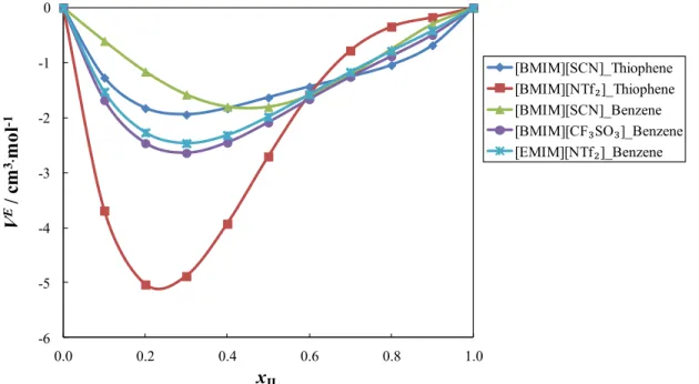
eye.__________________________________________________________________________ 69 Figure 3.1.3 - Excess molar volumes as a function of the mole fraction of the IL, in mixtures of [BMIM][SCN] with benzene, at different temperatures, namely, (u) 298.15 K, (p) 308.15
K, (n) 318.15 K and (l) 328.15 K. Solid lines represent the corresponding correlation of
Redlich-Kister. The dotted line corresponds to the limit of miscibility, where at the left is the immiscibility region. ___________________________________________________________75 Figure 3.1.4 - Estimated excess molar volumes through Redlich-Kister’s correlation as function of the mole fraction of the IL, at 298.15 K. _________________________________ 75 Figure 3.1.5 - Viscosity deviations as a function of the mole fraction of the IL, in mixtures of [BMIM][SCN] with thiophene, at different temperatures, namely, (u) 298.15 K, (p) 308.15 K, (n) 318.15 K and (l) 328.15 K. Solid lines represent the corresponding correlation of Redlich-Kister. The dotted line corresponds to the limit of miscibility, where at the left is the immiscibility region. ___________________________________________________________ 76 Figure 3.1.6 - Estimated viscosity deviations through Redlich-Kister’s correlation as function of the mole fraction of the IL, at 298.15 K. _________________________________________76
Figure 3.1.7 - 1H NMR chemical shift deviations for [BMIM][SCN] in the mixture with
thiophene. The dotted lines represent the hydrogen chemical shifts deviations for thiophene and full lines for the cation [BMIM]+. _____________________________________________80
Figure 3.1.8 - 13C NMR chemical shift deviations for [BMIM][SCN] in the mixture with
thiophene. The dotted lines represent the carbon chemical shifts deviations for thiophene, full lines for the cation [BMIM]+ and dashed lines for the anion [SCN]-. ___________________ 80
Figure 3.1.9 - 1H NMR chemical shift deviations for [BMIM][NTf
2] in the mixture with
thiophene. The dotted lines represent the hydrogen chemical shifts deviations for thiophene and full lines for the cation [BMIM]+. _____________________________________________81
Figure 3.1.10 - 13C NMR chemical shift deviations for [BMIM][NTf2] in the mixture with
thiophene. The dotted lines represent the carbon chemical shifts deviations for thiophene, full lines for the cation [BMIM]+ and dashed lines for the anion [NTf2]-. ___________________ 82
Figure 3.1.11 - Radial distribution functions of selected carbon atoms of a) [BMIM]+ around
the S atom of thiophene, b) thiophene atoms around the S atom of [SCN]-, in the system [BMIM][SCN] + thiophene. _____________________________________________________84 Figure 3.1.12 - Radial distribution functions of a) selected carbon atoms of [BMIM]+ around
the S atom of thiophene and b) thiophene atoms around the C1 atom of [NTf2]-, in the system
[BMIM][NTf2] + thiophene. _____________________________________________________ 85
Figure 3.1.13 - Spatial distribution functions (SDF) for [SCN]- (a, b) and [BMIM]+ (c) around thiophene from MD simulation of the [BMIM][SCN] + thiophene mixture. Yellow and blue regions represent SDF (isovalue = 25) for S and N atoms from the IL anion, respectively. Mauve, orange and brown regions represent SDF (isovalue = 32) for C10, C4 and C6 atoms of the IL cation, respectively. ____________________________________________________ 85 Figure 3.1.14 - Spatial distribution functions (SDF) for [NTf2]- (a, b) and [BMIM]+ (c) around
thiophene from MD simulation of the [BMIM][NTf2] + thiophene mixture. White and red
regions represent SDF (isovalues are 25 in a and 20 in b, respectively) for C and O atoms from the IL anion, respectively. Blue, orange and brown regions represent SDFs (isovalue = 32) for N2, C4 and C6 atoms of the IL cation, respectively. ___________________________86 Figure 3.1.15 - Atomic hits for SCN-constituting atoms at a) 2.5 Å, b) 3.0 Å and c) 3.5 Å around thiophene from MD simulation of the [BMIM][SCN] + thiophene mixture. Yellow, blue, cyan and white spheres stand for sulfur, nitrogen, carbon and hydrogen atoms, respectively. __________________________________________________________________ 88 Figure 3.2.1 - Chemical structures of the ions composing the studied ILs. _______________ 96 Figure 3.2.2 - Experimental and predicted water activity coefficients, at 298.2 K. Symbols are representing experimental data and full lines the COSMO-RS predictions (●,▬)
[BMIM][DCA], (u,▬) [BMIM][SCN], (■,▬) [BMIM][TCN] and (▲,▬) [EMIM][TCB]. The dashed lines for [BMIM][TCN] and [EMIM][TCB] indicate the immiscibility region of these ILs in water. _________________________________________________________________104 Figure 3.2.3 - Sigma profile for (▬) water, (▬) [DCA]-, (▬) [SCN]-, (▬) [TCN]-, (▬) [TCB]-,
(▬ ▬) [BMIM]+ and(▬ ●) [EMIM]+. ____________________________________________105 Figure 3.2.4 - Contribution of specific interaction to the total excess enthalpy, at xw = 0.5 and
T = 298.15 K. The contribution of excess enthalpies from electrostatic/misfit is represented by the blue bars, hydrogen bonding through the red bars, van der Waals through the green bars, and total excess enthalpies of the mixtures by the purple bars. __________________ 107 Figure 3.2.5. Radial distributions functions (RDFs) for mixtures of [BMIM][SCN] and water, at different mole fractions of IL and 298.15 K. RDFs for interaction of cation-water (H1-OW, ▬), anion-water (N-HW, ▬), cation-anion (H1-N, ▬) and solvent-solvent (OW-OW, ▬) are represented in each panel. _____________________________________________________ 109 Figure 3.2.6. Radial distributions functions (RDFs) for a) anion-water, b) cation-water, c) cation-anion and d) water-water interactions, at 80IL:20W and 298.15 K. RDFs for [BMIM][SCN] (▬), [BMIM][DCA] (▬), [BMIM][TCN] (▬) and [EMIM][TCB] (▬) are represented in each panel. _____________________________________________________ 110 Figure 3.2.7 - Spatial distribution functions (SDF) obtained by TRAVIS72, for the mixture
[BMIM][SCN] (above, left side), [BMIM][DCA] (above, right side), [BMIM][TCN] (down, left side) and [EMIM][TCB] (down, right side) and water, at 80IL:20W. Each anion is the
center element, surrounded by oxygen atoms of water (blue
surface)._____________________________________________________________________115 Figure 3.3.1 - Isobaric temperature-composition diagram of (a) [BMIM][SCN]+water, (b) [BMIM][DCA]+water, (c) [BMIM][TCN]+water, (d) [EMIM][TCB]+water. The solid lines represent COSMO-RS predictions. ______________________________________________131 Figure 3.3.2 - Isobaric temperature-composition diagram of (a) [BMIM][SCN]+ethanol, (b) [BMIM][DCA]+ethanol, (c) [BMIM][TCN]+ethanol, (d) [EMIM][TCB]+ethanol. The solid lines represent COSMO-RS prediction. __________________________________________ 132 Figure 3.3.3 - Radial distributions functions (RDFs) for a) [BMIM][SCN], b) [BMIM][DCA], c) [BMIM][TCN] and d) [EMIM][TCB], at 0.20 (on the left side) and 0.40 (on the right side) mole fraction of IL and 298.15 K. In each picture is represented all types of interaction, namely RDFs for anion-ethanol (▬), cation-ethanol (▬), cation-anion (▬) and ethanol-ethanol (▬) interactions. ______________________________________________________ 142 Figure 3.3.4 - Spatial distribution functions (SDFs) obtained by TRAVIS83, for the mixture [BMIM][SCN] (above, left side), [BMIM][DCA] (above, right side), [BMIM][TCN] (down,
left side) and [EMIM][TCB] (down, right side) and ethanol, at 0.20 mole fraction of IL. Each anion is the center element, surrounded by ethanol molecules (pink surface). ___________146 Figure 3.4.1 - Atom labels used in this work for glucose. ____________________________ 156 Figure 3.4.2 - Probability distribution of the hydroxymethyl group angle in glucose as a function of concentration.______________________________________________________ 159 Figure 3.4.3 - Comparison of experimental36 and simulation density values at 303.15 K. __160
Figure 3.4.4. Comparison of experimental36 and simulation viscosity values at 313.15 K. _ 163
Figure 3.4.5 - Radial distributions functions (RDFs) for glucose-water interactions, at six different glucose mole fraction and a temperature of 313.15 K. RDFs for interaction between O1-OW (▬), O2-OW(▬), O3-OW(▬), O4-OW (▬), O5-OW (▬) and O6-OW (▬) are represented in each figure. _____________________________________________________ 166 Figure 3.4.6 - Spatial distribution functions (SDFs) as a function of glucose concentration. A glucose molecule is the central element, surrounded by oxygen atoms of water (red surface)._____________________________________________________________________169 Figure 3.4.7 - The number of hydrogen bonds between glucose and water molecules (red, right axis) and water with water molecules (blue, left axis) as function of glucose concentration, at 313.15 K. _____________________________________________________170 Figure 3.4.8 - Comparison of experimental36 (line series) and simulation density values
estimated with scaled charges (dot series) and with the original charges (dotted-line series) at 313.15 K. ____________________________________________________________________172 Figure 3.4.9 - Comparison of experimental36 (line series) and simulation viscosity values estimated with scaled charges (dotted series) and with the original charges (dotted-line series) at 313.15 K. __________________________________________________________________172 Figure 3.5.1 – The solubility of glucose in water, [EMIM][SCN], [EMIM][DCA], [EMIM][TCN] and [EMIM][TCB], in a temperature range of (283.15 – 333.15) K. ______186 Figure 3.5.2 – Effect of different alkyl chain length of IL’s cation on glucose solubility, in a temperature range of (283.15 – 333.15) K. ________________________________________187 Figure 3.5.3 – Comparison of experimental and computed density, for systems composed of glucose and [EMIM][SCN] and [EMIM][DCA], at 313.15 K. ________________________189 Figure 3.5.4 – Comparison of experimental and computed viscosity, for systems composed of glucose and [EMIM][SCN] and [EMIM][DCA], at 313.15 K. ________________________ 189 Figure 3.5.5 – Atom labels used in this study for glucose. ____________________________191 Figure 3.5.6 - Radial distributions functions (RDFs) for water (above row), glucose-[EMIM][SCN] (middle row) and glucose-[EMIM][DCA] (bottom row) interactions, at six different glucose mole fraction and a temperature of 313.15 K. RDFs for interaction between
OW/N-HO12(▬), OW/N-HO8(▬), OW/N-HO6(▬), OW/N-HO4(▬), OW/N-HO2 (▬) are
represented in this figure. ______________________________________________________193 Figure 3.5.7 - Spatial distributions functions (SDFs) for water and glucose-anion/cation interactions, at six different glucose mole fraction and a temperature of 313.15 K. The central molecule is glucose, surrounded by water molecules (red surfaces), cations of IL (mauve surfaces) and anions of IL (blue surface). Isovalues for atoms in water and ILs are 36 and 7 particle·nm-‐3, respectively.______________________________________________196
Figure 3.5.8 - Radial distributions functions (RDFs) and Spatial distribution functions for glucose-anion interactions for the anions of CN-based ILs, at infinite dilution and a temperature of 313.15 K. RDFs for interaction between [EMIM][SCN](▬), [EMIM][DCA](▬), [EMIM][TCN](▬) and [EMIM][TCB](▬) with glucose are represented in this figure. Additionally, at SDFs, the mauve surfaces represent the cations, and the blue surfaces the anions surrounding a glucose molecule. ________________________________199 Figure 3.5.9 - Radial distributions functions (RDFs) and Spatial distribution functions for glucose-anion interactions for the anions of CN-based ILs and [EMIM][Ac], at different glucose concentrations and a temperature of 313.15 K. RDFs for interaction between [EMIM][SCN](▬), [EMIM][DCA](▬), and [EMIM][Ac](▬) with glucose are represented in this figure. Additionally, at SDFs, the blue surfaces represent the acetate anion surrounding a glucose molecule. _____________________________________________________________ 202
List of Tables
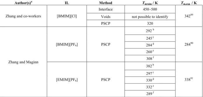
Table 2.1.1 - Detailed information concerning the MD simulations of studies reviewed in this section. ______________________________________________________________________ 26 Table 2.1.1.1 - Estimated densities by means of MD simulations and experimental data, at different temperatures. _________________________________________________________32 Table 2.1.2.1 - Comparison of estimated melting points obtained using different methodologies and MD simulations, Tm,sim, with available experimental, Tm,exp, data. ______35
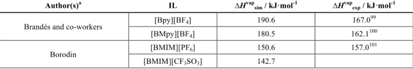
Table 2.1.3.1 - Calculated and Experimental Enthalpies of Vaporization, at T=298 K, for several ILs.___________________________________________________________________ 37 Table 2.1.4.1 - Estimated viscosities, at different temperatures, determined by means of MD simulations. ___________________________________________________________________41 Table 2.1.5.1 - Estimated diffusion constants, at different temperatures, determined by means of MD simulations._____________________________________________________________ 43 Table 2.1.2 - Accuracy of MD simulations for calculating structural and thermodynamic properties of ILs with respect to available experimental results. _______________________50 Table 3.1.1 - Experimental density as function of temperature for pure ionic liquids, thiophene, benzene and for their mixtures, in different mole fractions and at atmospheric pressure. ____________________________________________________________________ 69 Table 3.1.2 - Experimental viscosity data as function of temperature for pure ionic liquids, thiophene, and benzene, and also for their mixtures, in different mole fractions and at atmospheric pressure. __________________________________________________________72 Table 3.1.3 - Coefficients for Redlich-Kister correlations for excess molar volume. _______77 Table 3.1.4 - Coefficients for Redlich-Kister correlations for viscosity deviations. ________ 77 Table 3.2.1 - Experimental water activities (aw) and experimental and COSMO-RS water
activity coefficients (γw) in the binary mixtures at T = 298.2 K. _______________________ 102
Table 3.2.2 - Coordination number (Z) from the RDF peaks at distance below rZ nm for
anion-solvent, cation-solvent, cation-anion and solvent-solvent interaction, at each considered system and different IL mole fraction.____________________________________________112 Table 3.3.1 - Experimental isobaric VLE data for the system [BMIM][SCN] (1) + water (2)21
at (0.1, 0.07 and 0.05) MPa pressures. ____________________________________________134 Table 3.3.2 - Experimental isobaric VLE data for the system [BMIM][DCA] (1) + water (2) at (0.1, 0.07 and 0.05) MPa pressures. ______________________________________________ 134 Table 3.3.3 - Experimental isobaric VLE data for the system [BMIM][TCN] (1) + water (2) at (0.1, 0.07 and 0.05) MPa pressures. ______________________________________________ 135
Table 3.3.4 - Experimental isobaric VLE data for the system [BMIM][TCN] (1) + water (2) at (0.1, 0.07 and 0.05) MPa pressures. ______________________________________________ 136 Table 3.3.5 - Experimental isobaric VLE data for the system [BMIM][SCN] (1) + ethanol (2) at temperature T, liquid mole fraction x, at various system pressure 0.1, 0.07 and 0.05 MPa.________________________________________________________________________136 Table 3.3.6 - Experimental isobaric VLE data for the system [BMIM][DCA] (1) + ethanol (2) at temperature T, liquid mole fraction x, at various system pressure 0.1, 0.07 and 0.05 MPa.________________________________________________________________________137 Table 3.3.7 - Experimental isobaric VLE data for the system [BMIM][TCN] (1) + ethanol (2) at temperature T, liquid mole fraction x, at various system pressure 0.1, 0.07 and 0.05 MPa.________________________________________________________________________138 Table 3.3.8 - Experimental isobaric VLE data for the system [EMIM][TCB] (1) + ethanol (2) at temperature T, liquid mole fraction x, at various system pressure 0.1, 0.07 and 0.05 MPa.________________________________________________________________________139 Table 3.3.9 - Coordination number (Z) from the RDF peaks at distance below rZ nm, for
anion-ethanol, cation-ethanol, cation-anion and ethanol-ethanol interactions, at each system and different IL mole fraction, addressed in this study.______________________________144 Table 3.4.1 - Experimental36 and computational densities (ρ) for different glucose/water
mixtures at 303.15 K. Values in parentheses denote the uncertainties (the standard deviation) estimated with the calculated results. AAD represents the absolute deviations of the simulated data from the experimental values. ______________________________________________ 161 Table 3.4.2 - Experimental36 and calculated viscosities (η) at 313.15 K. Values in parentheses
denote uncertainties estimated accordingly to equation 3.4.3. AAD represents the absolute deviations of the simulated data from the experimental values. _______________________163 Table 3.4.3 - Computed self-diffusion coefficients at 313.15 K. Values in parentheses denote uncertainty (the standard deviation) associated with the calculated data. ______________ 164 Table 3.4.4 - Coordination number (CN) from the RDF peaks for glucose-water interactions, at each mixture considered. ____________________________________________________ 167 Table 3.5.1 – Coordination numbers (Z) from the RDFs peaks for glucose-water (OW
-HOglucose) and anion-glucose, at each mixture considered. ____________________________194
Table 3.5.2 – Number of hydrogen bonds established between glucose and water, [EMIM][SCN], [EMIM][DCA] and [EMIM][Ac], at two different glucose concentrations, at 313.15 K. ____________________________________________________________________197 Table 3.5.3 – Numerical values for the enthalpies calculated by Gaussian code, at gas phase
List of Symbols
aw Activity (of water)
kB Boltzmann Constant
δ Chemical Shift
Δδ Chemical Shift Deviation
Z Coordination Number
A Correlation/Fitting Parameter at equation 3.1.3 and 3.4.2/3
rZ Cutoffs
CN Cyano
H Enthalpy
ΔHvap Enthalpy of Vaporization
VE Excess Volume
G Free Energy of Gibbs
R Ideal Gas Constant
jxz Imposed Momentum Flux
L Length of the simulation box
Tm Melting Temperature/Point
x Molar fraction
U Molar Internal Energy
M Molecular weight
Pxx , Pxz Pressure Tensor (at different coordinates)
D Self-diffusion/ Diffusion Coefficient
T Temperature
t Time
ptotal Total Exchanged Momentum
∆η Viscosity Deviation, Viscosity Uncertainty - equation 3.4.3
V Volume
DNS 3,5-dinitrosalycilic acid
Greek Letters
ρ Density
α Fitting Parameter at equation 3.4.2/3
τ Fitting Parameter at equation 3.4.2/4
β Solvatochromic Parameter
γ Surface Tension, Activity Coefficient
Chemical Formulas
Ionic liquids
[EOHMIM][BF4] 1-(2-hydroxyethyl)-3-methylimidazolium tetrafluoroborate [OOHMIM][BF4] 1-(8-hydroxyoctyl)-3-methylimidazolium tetrafluoroborate [BMpyr][NTf2] 1-butyl-1-methylpyrrolidinium bis(trifluoromethanesulfonyl)imide [BMIM][Ac] / [BMIM][OAc]
/ [BMIM][C1CO2] 1-butyl-3-methylimidazolium acetate
[BMIM][NTf2] 1-butyl-3-methylimidazolium bis(trifluoromethylsulfonyl)imide [BMIM][Pf2] 1-butyl-3-methylimidazolium bis[(perfluoroethyl)sulfonyl]imide [BMIM][Br] 1-butyl-3-methylimidazolium bromide
[BMIM][Cl] 1-butyl-3-methylimidazolium chloride [BMIM][DCA] 1-butyl-3-methylimidazolium dicyanamide [BMIM][PF6] 1-butyl-3-methylimidazolium hexafluorophosphate [BMIM][I] 1-butyl-3-methylimidazolium iodide
[BMIM][CH3SO4] 1-butyl-3-methylimidazolium methane sulfate [BMIM][C1SO3] 1-butyl-3-methylimidazolium methylsulfonate [BMIM][NO3] 1-butyl-3-methylimidazolium nitrate
[BMIM][BF4] 1-butyl-3-methylimidazolium tetrafluoroborate [BMIM][SCN] 1-butyl-3-methylimidazolium thiocyanate [BMIM][TOS] 1-butyl-3-methylimidazolium tosylate
[BMIM][TCN] 1-butyl-3-methylimidazolium tricyanomethane [BMIM][CF3CO2] 1-butyl-3-methylimidazolium trifluoroacetate
[BMIM][CF3SO3] 1-butyl-3-methylimidazolium trifluoromethanesulfonate [pyr14][NTf2] 1-butyl-3-methylpyridinium bis(trifluoromethylsulfonyl)imide [C10MIM][NTf2] 1-decyl-3-methylimidazolium bis(trifluoromethylsulfonyl)imide [C12MIM][NTf2] 1-dodecyl-3-methylimidazolium bis(trifluoromethylsulfonyl)imide [EMIM][Ac] 1-ethyl-3-methylimidazolium acetate
[EMIM][NTf2] 1-ethyl-3-methylimidazolium bis(trifluoromethylsulfonyl)imide [EMIM][Br] 1-ethyl-3-methylimidazolium bromide
[EMIM][Cl] 1-ethyl-3-methylimidazolium chloride [EMIM][DCA] 1-ethyl-3-methylimidazolium dicyanamide [EMIM][C2H5SO4] 1-ethyl-3-methylimidazolium ethylsulfate
[EMIM][PF6] 1-ethyl-3-methylimidazolium hexafluorophosphate [EMIM][NO3] 1-ethyl-3-methylimidazolium nitrate
[EMIM][TCB] 1-ethyl-3-methylimidazolium tetracyanoborate [EMIM][BF4] 1-ethyl-3-methylimidazolium tetrafluoroborate [EMIM][SCN] 1-ethyl-3-methylimidazolium thiocyanate [EMIM][TOS] 1-ethyl-3-methylimidazolium tosylate
[EMIM][TCN] 1-ethyl-3-methylimidazolium tricyanomethane
[EMIM][CF3SO3] 1-ethyl-3-methylimidazolium trifluoromethanesulfonate [EMpy][C2H5SO4] 1-ethyl-3-methylpyridinium ethylsulfate
[HMIM][NTf2] 1-hexyl-3-methylimidazolium bis(trifluoromethylsulfonyl)imide [HMIM][Cl] 1-hexyl-3-methylimidazolium chloride
[HMIM][PF6] 1-hexyl-3-methylimidazolium hexafluorophosphate [HMIM][I] 1-hexyl-3-methylimidazolium iodide
[BMpy][BF4] 1-methyl-3-butylimidazolium tetrafluoroborate
[EMIM][N(SO2CF3)2] 1-methyl-3-ethylimidazolium bis(trifluoromethane)sulfonamide [patr][Br] 1-n-butyl-4-amino-1,2,4-trizolium bromide
[OMIM][NTf2] 1-octyl-3-methylimidazolium bis(trifluoromethylsulfonyl)imide [OMIM][PF6] 1-octyl-3-methylimidazolium hexafluorophosphate
[OMIM][I] 1-octyl-3-methylimidazolium iodide
[OMIM][BF4] 1-octyl-3-methylimidazolium tetrafluoroborate
[C14MIM][NTf2] 1-tetradecyl-3-methylimidazolium bis(trifluoromethylsulfonyl)imide [(OCH3)2C1im][PF3(C2F5)3] 1,3-dimethoxy-2-ethylimidazolium tris(pentafluoroethyl)trifluorophosphate [DMIM][NTf2] 1,3-dimethylimidazolium bis(trifluoromethanesulfonyl)imide
[DMIM][Cl] 1,3-dimethylimidazolium chloride
AP-N acyclic pentamethylpropylguanidinium nitrate AP-C acyclic pentamethylpropylguanidinium perchlorate CM-N cyclic tetramethylguanidinium nitrate
[N4111][NTf2] N-butyl-N,N,N-trimetylammonium bis(trifluoromethanesulfonyl)imide [Bpy][BF4] n-butylimidazolium tetrafluoroborate
[Bpy][Cl] n-butylpyridinium chloride
[K][N(SO2C2F5)2] potassium cis-bis(perfluoro-n-butylsulfonyl)amide [Na][N(SO2C2F5)2] sodium trans-bis(perfluoro-n-butylsulfonyl)amide [P6 6 6 14][OAc] tetradecylphosphonium acetate
[P 10 10 10 10][Br] tetradecylphosphonium bromide
[P6 6 6 14][CF3SO3] tetradecylphosphonium trifluoromethanesulfonate
[P6 6 6 14][NTf2] tetradecyltrihexylphosphonium bis(trifluoromethanesulfonyl)imide [N 1 1 1 1][DCA] tetramethylammonium dicyanamide
[PH(C6H5)3][N(SO2F)2] triphenylphosphonium bis(fluorosulfonyl)amide
Other compounds CO2 Carbon Dioxide CO Carbon Monoxide H2 Hydrogen (gas) H2O2 Hydrogen Peroxide CH4 Methane NOX Nitrogen Oxide N2O Nitrous Oxide SO2 Sulfur Dioxide SOX Sulfur Oxide
Subscripts
exp experimental glucose
i specie
IL Ionic Liquid
L length of the simulation box
m melting max mix mixture pure ref reference sim simulation total w, water water Superscripts cohesive E excess
gas gas phase
liq liquid phase vap vaporization
1.1.
Scope and Objectives
Unlike the expectations of many, fossil fuels are today, and will remain for long, our main source of energy and transport fuel1. Nevertheless, the environmental impact of their continued usage is well known by the emission of pollutant gases released during their combustion with concomitant extremely severe climatic consequences. Emissions of NOX (nitrogen oxides), SOX (sulfur oxides), CO2, N2O and CH4 are some of the most harmful gases responsible for acid rain and greenhouse effects, having also a significant negative impact on human health1. For this reason, there is a worldwide concern in reducing the high dependence on fossil fuels by replacing them for other alternatives, such as biofuels, as well as continuing to develop and improve technologies to reduce the emission of harmful gases from their combustion.
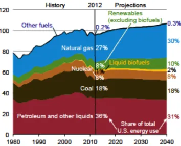
Figure 1.1 - Primary energy use in the U.S.A since 1980 and projections up to 2040. Energy Information Administration (EIA), Monthly Energy Review, September 2013, DOE/EIA-0035 (2013/09).2
Environmental regulations at different countries have imposed stringent rules, aiming at the reduction of SOX emissions (responsible for acid rains and also for poisoning the catalytic activity implemented on motor engines), requiring refineries to produce fuels with ultra-low sulfur content of 10 ppm according to EU and US legislation2,3. At the same time, alternatives to the use of fossil fuels have gained an interesting place, with a prediction for concomitant increases in their usage and for important investments in the next decades (Figure 1.1). Within the possible alternatives, biofuels seem to be one of the most promising options, becoming the object of a significant number of studies
devoted to their production, such as bioethanol and biodiesel, through processes based on the consumption of biomass (renewable material). Albeit biofuels eliminate the emission of harmful gases, their production still requires a lot of attention, either from academia and industry, since they are not yet economic and sustainable alternatives.4
For the last decades, for both fuel improvement and biofuel production processes, a new class of solvents named ionic liquids (ILs)5 has been studied and applied. These solvents are molten salts, that have attracted a lot of attention from academia and industry due to their unique properties, including a fine-tuning ability when combining different cations and anions, aimed for a specific application.6 Considering the chemical industry, such as fuel and biofuel industries, the ILs have gained an interesting role acting as extractive solvents, by presenting attractive physicochemical properties which enable optimization of processes, as well as, reduction of operational costs.7
Predictive approaches, namely, methods based on equations of state (EoS), quantitative structure – property/activity relationships (QSPR/QSAR), and computer approaches (e.g. quantum density functional and wavefunction method, or classical molecular dynamics or Monte Carlo simulations) have been used to understand the behavior of ILs at different working conditions. Molecular dynamics (MD) simulation stands out by its ability to reproduce the dynamics of real systems, allowing to evaluate and estimate properties at the microscopic level.8 Additionally, the reproduction of systems composed of ILs by means of MD simulation is a hot topic in scientific research. High viscosity and high ability to solubilize a wide range of compounds are some of the motivations for developments and improvements of computer and molecular approaches.7
Hereafter, this thesis is devoted to investigate the role and the mechanisms of ILs, acting as solvent, by means of MD simulations, in systems relevant for fuel and biofuel productions, and at biomass pre-treatment processes. With this aim simulations are performed for the characterization of binary systems composed of ILs and thiophene, benzene, ethanol or water (compounds of interest in fuel or biofuels streams), and also with glucose molecules (reproducing the existent interactions in pre-treatment processes of lignocellulosic materials for bioethanol production). After characterizing the systems, a general discussion is presented on how ILs interact with the various target compounds, including the mechanisms, type and strength of those interactions, aiming at an evaluation of their applicability in fuels and biofuels streams, as well as, for biomass pre-treatment processes.
Having defined the main objectives of this thesis, this chapter is going to briefly address the following issues: ILs and their main characteristics (Chapter 1.2), desulfurization processes and the role of ILs in this topic (Chapter 1.3), and biofuel production, emphasizing the second generation biofuels and processes of lignocellulosic material’s pre-treatment (Chapter 1.4). In Chapter 2, it is
going to be presented and compared the available computational approaches, highlighting the molecular dynamics simulation and its usage in the prediction of ILs’ properties. The Chapter 3 contains the description of the work performed, namely, the characterization of binary systems composed of ILs and thiophene or benzene, ILs and water or ethanol, and finally, glucose-based systems. The final chapter of this document will include a general discussion of the results obtained and will end with the conclusions.
1.2.
Ionic Liquids (ILs)
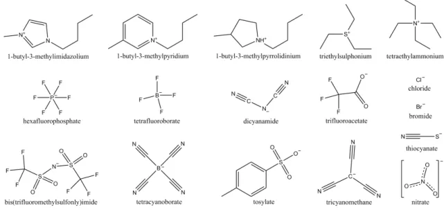
In the early 20th century, a new generation of molten salts was discovered by Paul Walden5. These molten salts are known by different names, such as ionic melts, ionic fluids, or liquid electrolytes but the most common and better recognized designation is ionic liquids. 9 These compounds possess at least one asymmetric unit comprised of a large organic cation, e.g. derived from imidazolium, pyridinium, pyrrolidinium, ammonium or phosphonium, and an organic or inorganic anion, such as bis[(trifluoromethyl)sulfonyl]imide, trifluoromethylsulfonate, hexafluorophosphate, or tetrafluoroborate. Examples of the structures of common cations and anions are shown in Figure 1.2.1.9,10
Figure 1.2.1 - Common cations and anions found in ionic liquids literature.
The structural asymmetry makes difficult their crystallization and minimizes the cation-anion interaction, which confers unique properties to ILs. They possess low melting point (<100 °C),
extremely low vapor pressure, high thermal and chemical stability, high ionic conductivity and good solvating capacity for organic and inorganic compounds and even biopolymers (cellulose). Furthermore, ILs are in general non-flammable and present a very broad liquidus temperature range. Moreover, it is possible to tune their properties by changing their constituting ions, within the large number of possible combinations of cations and anions, and by adding specific functional groups in order to achieve the desired physicochemical properties intended for a specific application. Given the possibility of fine-tuning the properties of ILs, their range of applicability is vast. Separation processing, chemical processing, biotechnology, electrochemistry are some of the possible application fields where ILs may act, for example, as solvents, lubricants, electrolytes or heat transfer fluids.6,9 Although ILs appeared to be an alternative to replace common solvents, as for example the volatile organic compounds, VOCs, due to their “greener” character when compared with that of the latter, parameters such as toxicity and biodegradability have been lately a matter of concern.11–13 Moreover, the viscosity of ILs is considered one of the main drawbacks for their application at industrial scale, with values reaching 100-1000 cP, i.e., one hundred to one thousand times larger than the viscosity of water.14 Polarity and ionization are other topics of interest and importance which are also discussed.10
The properties of ILs are greatly influenced by the structural specificities of their constituting cations and anions. The knowledge of the structure-property relationships of ILs is required for the selection or design of an IL for a specific application. Thus, information regarding some properties such as densities, viscosities, diffusivities, melting points or electric conductivities of as many ILs as possible is needed. However, the considerable number of potential cation/anion combinations makes this task daunting by an experimental approach alone. In an attempt to relate structure with property, group contribution methods and QSPR/QSAR (quantitative structure – property/activity relationships) approaches have been used to predict thermophysical properties, phase behaviors, toxicities, among others, of some ILs15–18. A review 19 on these types of methods for the estimation of thermophysical and transport properties of ionic liquids has been published. Also for the same purpose, quantum methods and statistical mechanics-based molecular approaches are gaining importance in this field since they have been helping to better understand, at the molecular level, the structure-property relationships and phase behavior of neat IL and IL in mixtures (with one or more compounds).20–24 Inherent to the nature of each moiety is the nature of its self-organization, and its influence on their properties, especially on their performance as solvents, which is a theme of a growing relevance. Canongia-Lopes and co-workers25–27 are among the pioneering researchers to show that the bulk liquid phase of ILs present a structure characterized by two main domains, a polar (high-charge density part composed by a hydrophilic head-group) and a non-polar (low-charge density part composed by a
hydrophobic tail) domains, at nanometer scale, which have been widely used to justify different behaviors (and properties) of ILs.10 In a different study28, it was possible to conclude that due to this unique structure, ILs present a “chameleonic behavior”, a sort of amphiphilic character that allows their simultaneous interaction with two compounds of different polarities. The so-called chameleonic behavior is just an example of how ILs can be complex solvents and, thus, their characterization opened a new and interesting research field.
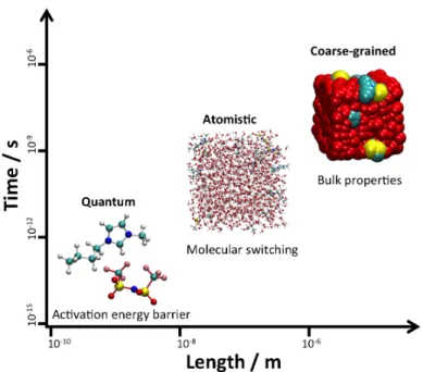
In this matter, in the past few years, several works including some extended studies or reviews10,29,30 have been addressing the application of computational approaches to model neat ILs and also mixtures of ILs. Ab initio methods, Monte Carlo (MC) and molecular dynamics simulations employing atomistic or coarse-grained (CG) models, are computer approaches that are being widely used to investigate these systems at different time and length scales.31–34 These different approaches are going to be briefly introduced in Chapter 2. Furthermore, focusing on MD simulations, an overview of methodologies applied to predict properties of neat ILs, namely, density, viscosity, diffusivity, melting point, vapor pressure and boiling point, enthalpy of vaporization and surface tension, will be presented.
1.3.
Fossil fuels improvement – desulfurization processes
One way to reduce the emission of pollutant gases is to remove the sulfur-content from petroleum, through desulfurization processes. The most common desulfurization process applied on refineries is hydrodesulfurization (HDS). In this process, refined petroleum is submitted to high pressures (20 - 100 bar of H2) and temperatures (300 - 400 oC) conventionally mediated with CoMo and NiMo-based catalysts.1,35,36 Refined petroleum includes different aliphatic and aromatic sulfur-based compounds where some, like benzothiophene (BT), dibenzothiophene (DBT) and their derivatives, are resistant to HDS, due to steric hindrance. Therefore, in order to fulfill the increasing strictness of the environmental regulations, the HDS process demands more extreme operation conditions, being a disadvantage of its implementation.35 Additionally, another problem associated with the HDS process is that some of non-sulfur aliphatic compounds, important for fuel performance, are also removed. Another drawback that can be associated with the process is that the presence of sulfur containing compounds, along with aromatic and nitrogen-based compounds, can poison the activities of the catalysts employed in the HDS process, which is also important to avoid.1
Several processes have been developed and improved to successfully replace HDS aiming at reducing the sulfur content, namely, desulfurization by adsorption, extraction, oxidation and biodesulfurization.1,35,37–40
Desulfurization by adsorption can be divided in physical and chemical adsorption, or more specifically, adsorptive and reactive desulfurization, respectively. As the name indicates, adsorptive desulfurization is based on the simple adsorption (van der Walls interactions) of sulfur compounds to adsorbents, usually zeolites41,42, Ni-based adsorbents43, CoMo/alumina43 or even metal-organic frameworks (MOFs)44,45. As for reactive adsorption46, an adsorbent such as Ni-ZnO has the ability to adsorb and convert sulfur compounds to sulfides and hydrocarbons. Sulfides are retained at the adsorbent and upon its regeneration SOX species are released. Still, the adsorption capacity of these adsorbents can be limited, which also confines the applicability of these methods in fuel streams with high content of sulfur compounds.1,35
Desulfurization by oxidation is a two-step process.1,35,47 The first step is the oxidation of sulfur compounds upon contact with an oxidant, usually hydrogen peroxide (H2O2), to form sulfoxides or sulfones. The latter compounds possess higher polarities than the sulfur ones present in petroleum, so they can be separated through liquid-liquid extraction using acetonitrile, dimethylformamide (DMF) or dimethyl sulfoxide (DMSO) as solvents, or alternatively by adsorption. Acetonitrile is the most commonly used solvent, owing to its low boiling point that allows its separation from the sulfones by simple distillation. Desulfurization by oxidation, however, is able to remove simultaneously olefins, requiring the management of a significant amount of the formed sulfone compounds.
Biodesulfurization is based on the use of microorganisms that selectively oxidize sulfur atoms, in the presence of water and oxygen under room temperature and pressure conditions.1,35,48 However, only a few number of bacteria species can oxidize BT and just a single specie can deal with thiophene. In the case of DBT, it is not possible to achieve the intended sulfur content with biodesulfurization. Therefore, this methodology can only be applied as a complementary step of another process.
Desulfurization by extraction, also known as extractive desulfurization, is used as a complementary step to desulfurization by oxidation, or as a single process if low temperature and pressure conditions are considered.1,35 This process is based on the high affinity and selectivity of a chosen solvent to interact with the sulfur compounds, which should be more soluble in the solvent than in the hydrocarbons present in the fuel. After solubilization, the solvent should be easily separated from the sulfur compounds by simple distillation, through the difference of the boiling temperatures. To attain an efficient process, the choice of the solvent must be adequate. Solvents such as methanol, ethylene glycol, acetonitrile, DMF, DMSO and sulfolane can be used or, to enhance the solubility, a mixture of solvents. Another alternative is the use of the ILs.1,35–37,40
ILs have some advantages over conventional solvents, namely their low vapor pressure enhancing the separation from sulfur compounds through distillation, their thermal and chemical stability, as well
as a liquidus profile in a wide range of temperatures. Composed of a bulky organic cation and an organic/inorganic anion, they can be chosen accordingly to their properties to fulfill a specific application, as mentioned previously in Chapter 1.1.37 The selective sulfur removal is dependent on the size and structure of both cations and anions, as well as their affinity to different sulfur compounds, which is mainly made through π-π interactions, originally from their aromatic character. Regarding the cation’s families, imidazolium, pyridinium-based ILs and Lewis and Brønsted acidic ILs have been studied, where it was recognized a significant efficiency of sulfur removal with the increase of the length of alkyl chains. The Lewis and Brønsted acidic ILs, have an enhanced extraction power due to their capacity to form sulfur-complexes. Concerning the anions, tetrafluoroborate, hexafluorophosphate, octyl sulfate, ethyl sulfate and dimethyl phosphate are usually studied.1,35–37,40 Nevertheless, ILs of low viscosity that are composed of dicyanamide and thiocyanate anions, were also reported to have a good extraction performance, as well as, a significant selectivity under the presence of polyaromatic hydrocarbons also extracted from petroleum streams.1,35 Additionally, it has been reported that ILs, along with hydrogen peroxide (H2O2) and other catalysts, can achieve sulfur removal efficiencies around 98.2 %, proving that a combination of catalytic oxidation with an ionic liquid can lead to sulfur compounds content, at ambient conditions and without H2 consumption, in accordance with regulations.35
It is worth noting that, with the increase of petroleum exploration in the world, new sources of crude have been found, with significantly higher sulfur content, requiring an adjustment or a combination of different methods.1
1.4.
Biofuels
In order to replace fossil fuels, the production of biofuels appeared as one of the most promising alternatives. Biofuels are classified as first, second and third generation. First generation biofuels are those produced from sugar, starch, vegetable oils or animal’s fats, i.e., mainly from food crops and oil seeds. Biofuels of second generation are produced from lignocellulosic materials, such as wood process wastes, agricultural and forest residues, vegetative grasses and bagasse. Third generation biofuels are produced from algae. The two latest generations are non-food feedstocks, avoiding problems related to economic and social impacts. Nevertheless, for a sustainable replacement of fossil fuels, the production of biofuels should be an economic and sustainable option, with an availability of the feedstock as high as possible, and simultaneously be able to produce power and chemicals, which
may require high investments not only for the process, but also for storage and delivery of biofuels to its final destination.4,49
Hereafter, it will be emphasized the second generation biofuels production, addressing the processes of converting biomass in biofuel, and also the lignocellulosic material’s pre-treatment processes.
For the conversion of biomass into biofuels, two routes are adopted, namely the thermochemical and biochemical conversion. Thermochemical conversion processes include liquefaction, pyrolysis and gasification.4 Generally, the latter processes are based on a chemical change suffered by the lignocelllulosic material when heat is applied, in the absence or presence of oxygen. Changing the temperature, pressure, heating rate or time of gas residence, different final products can be obtained, from chemicals to hydrocarbons, bioethanol, biodiesel and heat. From gasification is also produced fuel gases and syngas (gas rich in H2, CO and CO2) that can be further used in the synthesis of long-chain hydrocarbons for producing high cetane number fuels (Fischer-Tropsch process).4,49–52
As for biochemical conversion processes, these are performed at low temperatures and low reaction rates, where enzymatic hydrolysis of hemicellulose and cellulose (wood’s constituents) are carried, followed by the fermentation of their small molecules that will give origin to biofuel.4,53,54 The definition of biochemical conversion process is commonly associated with bioethanol production, using lignocellulosic biomass. Nevertheless, the structural organization of lignocellulosic biomass compounds (cellulose, hemicellulose and lignin) is complex, which causes difficulties in the assessment of enzymes or acids to cellulose and hemicellulose and, consequently, hinders the process of fermentation to obtain bioethanol.55,56 To overcome this, pre-treatment processes (chemical, physical or biological) are required. The resulting sugars are then fermented and the ethanol produced is used as fuel, chemical or product.4
1.4.1. Lignocellulosic materials and pre-‐treatment processes
Carbohydrates are an amazing and diversified class of biomolecules, characterized by a vast heterogeneity of compounds differing on their stereochemistry and functionalization. These compounds are essential to many biological functions and are also applied in a wide range of industrial processes such as food, textile, pulp and paper, biofuels, and personal care/cosmetic industries.55,57,58
Wood is a renewable source of carbohydrates usually composed of 35-50% of cellulose, 35% of hemicelluloses, 5 - 30% of lignin and extractives. Cellulose is the most
abundant compound, characterized for being a homopolysaccharide composed of β-D-glucopyranose units, which are linked together through (1-4)-glycosidic bonds (see Figure 1.4.1.1) in a linear direction and also by intra and intermolecular hydrogen bonds.56,59
Figure 1.4.1.1 - Structure of cellulose.59
Cellulose molecules aggregate to microfibrils with highly ordered regions (crystalline) and less ordered regions (amorphous). Bundles of microfibrils compose fibrils, which comprise cellulose fibers. The crystalline region of cellulose can present different polymorphs, beginning with the native cellulose, cellulose I (Figure 1.4.1.2), characterized by cellulose microfibrils oriented in the same direction (parallel chains) and establishing van der Waals interactions between layers. The establishment of three characteristic hydrogen bonds between molecules is observed (two intramolecular hydrogen bonds and one intermolecular hydrogen bond), responsible for the ordered structure and for the lack of interactions with water and most of organic solvents. When cellulose is dissolved and then regenerated, the order of cellulose microfibrils is altered and additional hydrogen bonds are established between layers, which are now antiparallel chains. In this form, cellulose is usually named cellulose II.59 Other two polymorphs can be obtained by heating or chemical treatment, namely cellulose III and IV.59
Figure 1.4.1.2 – Projection of the plane in cellulose I, showing the hydrogen bonding network and the numbering of the atoms. Each glucose residue forms two intramolecular hydrogen bond (O3-H—05´ and O6—H-02´) and one intermolecular bond (O6-H—O3).59
Contrary to cellulose, hemicellulose is a heteropolysaccharide that can be composed of D-xylose, D-mannose, D-glucose or D-galactose monosaccharides connected linearly and/or with branches. According to its structure, hemicellulose is characterized by being an amorphous polymer, accessible to enzymatic attack, which enables hydrolysis and further conversion of its simple sugars. Hemicellulose and cellulose are embedded by another compound, lignin. Lignin is a complex, amorphous polymer composed of aromatic alcohols units, namely, coniferyl, sinapyl and p-coumaryl alcohols. The composition on wood of each of these compounds can vary, depending on the source of the wood.56,59
Aiming at separating cellulose, hemicellulose and lignin, mainly to obtain their monosaccharides for the production of biofuels, different solvents were studied and applied. Regarding cellulose dissolution, solvents such as carbon disulfide, LiCl-based solvents60, dimethylsulfoxide (DMSO)/paraformaldehyde61 and also N-methylmorpholine-N-oxide (NNMO)62 have been used. However, these solvents are volatile, toxic, expensive and difficult to recover.56
Figure 1.4.1.3 – Mechanism of pretreating lignocellulosic materials63.
Alternatively, and as mentioned previously, pre-treatment processes can be applied to biomass, being divided in biochemical, physical, biological and physicochemical pre-treatments.4,56,64,65 As Figure 1.4.1.3 illustrates, the aim of pre-treatment processes is to open the structure, breaking lignin and disrupting the crystalline structure of cellulose, promoting the accessibility of enzymes responsible for the hydrolysis of cellulose into its monosaccharides. These processes impose structural changes to the initial lignocellulosic biomass, but there are several factors that should be addressed. One factor to take into account is the composition of the biomass (in each of its three main constituents) which affects, accordingly, the choice of the most adequate pre-treatment process.64,65 Additionally, the process chosen should not degrade hemicellulose or cellulose, should not produce toxic compounds nor solid-waste residues, it must operate at reduced cost (either in heat and power demands), as well as with small enzyme dosages and short reaction times. Moreover, it should be possible to recover lignin, enhance fermentation process and finally, obtain high yields of sugars’ conversion.64
Biological pre-treatments employ microorganisms that will mainly attack hemicellulose and lignin, being a reduced cost procedure, with low energy consumption and mild operation conditions. However, the sugar conversion yield is usually low.64,65
Physical pre-treatments such as, extrusion and mechanical procedures can also be applied. These are based on the reduction of the particle size through milling or submitting the biomass to heat, mixing and shearing (extrusion process), which also disrupt the crystalline structure, and destroy fibers of biomass, enabling the enzymatic attack. Nonetheless, these processes require high power consumption.64,65


![Figure 3.1.2 - Liquid-liquid phase diagrams for [BMIM][NTf 2 ] (measured in this work), [BMIM][SCN] 18 and [BMIM][CF 3 SO 3 ] 19 with thiophene](https://thumb-eu.123doks.com/thumbv2/123dok_br/15951588.1097618/90.918.227.719.137.458/figure-liquid-liquid-phase-diagrams-bmim-measured-thiophene.webp)
![Figure 3.1.5 - Viscosity deviations as a function of the mole fraction of the IL, in mixtures of [BMIM][SCN]](https://thumb-eu.123doks.com/thumbv2/123dok_br/15951588.1097618/97.918.232.720.138.461/figure-viscosity-deviations-function-mole-fraction-mixtures-bmim.webp)