Reconstruction and identification of τ lepton decays to hadrons and ν$_τ$ at CMS

EUROPEAN ORGANIZATION FOR NUCLEAR RESEARCH (CERN)

CERN-PH-EP/2013-037 2016/02/22

CMS-TAU-14-001

Reconstruction and identification of τ lepton decays to

hadrons and ν

at CMS

The CMS Collaboration

Abstract

This paper describes the algorithms used by the CMS experiment to reconstruct and identify τ → hadrons+ντ decays during Run 1 of the LHC. The performance of the algorithms is studied in proton-proton collisions recorded at a centre-of-mass en-ergy of 8 TeV, corresponding to an integrated luminosity of 19.7 fb−1. The algorithms achieve an identification efficiency of 50–60%, with misidentification rates for quark and gluon jets, electrons, and muons between per mille and per cent levels.

Published in the Journal of Instrumentation as doi:10.1088/1748-0221/11/01/P01019.

c

2016 CERN for the benefit of the CMS Collaboration. CC-BY-3.0 license

∗_{See Appendix A for the list of collaboration members}

1

1

Introduction

Decays of τ leptons provide an important experimental signature for analyses at the CERN LHC. Evidence for decays of the standard model (SM) Higgs boson (H) into ττ has been re-ported [1, 2], as have searches for neutral and charged Higgs bosons in decays to τ leptons that have special interest in the context of the minimal supersymmetric extension of the SM (MSSM) [3–8]. The CMS collaboration has published analyses of Drell–Yan (qq→Z/γ∗ →ττ) and top quark pair production [9–11] in final states with τ leptons. Searches for supersymme-try, leptoquarks, W0 and Z0bosons, as well as other non-SM Higgs bosons [12–17] benefit from the high performance τ reconstruction and identification capabilities of the CMS detector. With a mass of mτ = 1.777 GeV [18], the τ is the only lepton heavy enough to decay into hadrons (h), and it does so in about two thirds of the cases, typically into either one or three charged pions or kaons and up to two neutral pions (π0), and one neutrino (ντ). The π0meson decays almost exclusively into γγ. In about 35% of the cases, τ leptons decay into an electron or muon and two neutrinos. The branching fractions for the main τ decay modes are given in Table 1. The decays τ− → h−π0ντ, τ− → h−π0π0ντ, and τ− → h−h

+_h−

ντ (with cor-responding channels for τ+_{) proceed via intermediate ρ(770)and a}

1(1260)meson resonances.

The electrons and muons originating from τ decays are difficult to distinguish from electrons and muons produced directly in the primary proton-proton (pp) interaction, and are handled using the standard CMS algorithms for electron and muon reconstruction and identification. The algorithms for τ reconstruction and identification presented in this paper focus on τ lep-ton decays to hadrons+ντ, that we refer to as “hadronic” τ decays and denote by τh. The

algorithms provide the means for reconstructing individually the dominant τhdecay modes.

In comparing the energies of reconstructed τ_hcandidates to their true energies, we refer to the charged hadrons and neutral pions produced in the τ decay as “visible” τ decay products, and ignore the ντ.

Table 1: Approximate branching fractions (B) of different τ decay modes [18]. The generic sym-bol h−represents a charged hadron (either a pion or a kaon). Charge conjugation invariance is assumed in this paper.

Decay mode Meson resonance B[%]

τ−→e−νeντ 17.8 τ−→µ−νµντ 17.4 τ−→h−ντ 11.5 τ−→h−π0ντ ρ(770) 26.0 τ−→h−π0π0ντ a1(1260) 9.5 τ−→h−h+h−ντ a1(1260) 9.8 τ−→h−h+h−π0ντ 4.8

Other modes with hadrons 3.2

All modes containing hadrons 64.8

The mean lifetime of τ leptons at rest is 290×10−15s [18]. The distances that τ leptons travel be-tween their production and decay are small, but nevertheless significant compared to the trans-verse impact parameter and secondary-vertex resolution of the CMS tracking detector [19]. En-ergetic τ leptons originating from Z or SM Higgs boson decays typically traverse distances of a few millimetres before decaying.

The main challenge in identifying hadronic τ decays is distinguishing them from quark and gluon jet background. The cross section for multijet production from perturbative quantum chromodynamical (QCD) calculations exceeds by many orders of magnitude the rate at which

τleptons are produced at the LHC. To reduce the background arising from quark and gluon jets, we exploit the fact that hadronic τ decays result in a lower particle multiplicity, and are more collimated and isolated relative to other particles in the event. In some analyses, the misidentification of electrons or muons as τ_h candidates may constitute a sizeable problem, and dedicated algorithms have been developed to reduce this type of background.

The performance of τh reconstruction and identification algorithms has been validated using

the first LHC data recorded at√s=7 TeV [20]. Since then, the algorithms have been further de-veloped, especially to improve their performance in dealing with additional inelastic pp inter-actions (pileup) that occur in the same bunch crossing as the hard scattering of interest. More-over, the rejection of backgrounds arising from misidentification of jets, electrons, and muons as τ_hhas improved significantly through the introduction of multivariate analysis (MVA) tech-niques. In this paper, we report on the performance of the improved algorithms used to analyze the 8 TeV pp data at CMS, corresponding to an integrated luminosity of 19.7 fb−1.

The paper is organized as follows. The CMS detector is described briefly in Section 2. Section 3 describes the data and the Monte Carlo (MC) simulations used for studying the performance of τhreconstruction and identification. The reconstruction of electrons, muons, and jets, along

with various kinematic quantities is described in Section 4. The algorithms used for reconstruc-tion and identificareconstruc-tion of τhdecays are detailed in Section 5. The performance of the algorithms

in simulated events is presented in Section 6. Sections 7–11 detail the validation of the algo-rithms with data. The results are summarized in Section 12.

2

CMS detector

The central feature of the CMS detector is a superconducting solenoid of 6 m internal diameter, providing a magnetic field of 3.8 T. A silicon pixel and strip tracker, a lead tungstate crystal electromagnetic calorimeter (ECAL), and a brass and scintillator hadron calorimeter (HCAL), each composed of a barrel and two endcap sections, are positioned within the solenoid volume. Muons are measured and identified in gas-ionization detectors embedded in the steel flux-return yoke outside the solenoid. Extensive forward calorimetry complements the coverage provided by the barrel and endcap detectors.

The CMS tracker is a cylindrical detector of 5.5 m length and 2.5 m diameter, constructed en-tirely of silicon modules. It provides an active sensor area of about 200 m2 to reconstruct charged particles within the pseudorapidity range |η| < 2.5. The innermost region around the interaction point, subject to the highest particle flux, is instrumented with silicon pixel sensors. The central part of the pixel detector consists of three cylindrical layers, installed at transverse radii of r = 4.4, 7.3, and 10.2 cm, which extend over a total length of 53 cm. The central part is complemented by two forward endcap disks of radius 6< r<15 cm, located at longitudinal distances|z| = 34.5 and 46.5 cm on either side of the interaction point. The cen-tral part of the silicon strip detector consists of ten cylindrical layers and twelve endcap disks that surround the pixel detector volume. The cylindrical layers cover radial distances of up to 108 cm and |z| < 109 cm, and the disks cover up to r < 113 cm and |z| < 280 cm. Tracks of charged hadrons are reconstructed with an efficiency of 75–95% that depends on the transverse momentum pT and η [21].

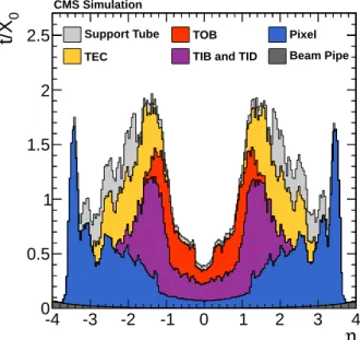
The silicon tracker adds a significant amount of material in front of the ECAL, mainly because of the mechanical structure, the services, and the cooling system. Figure 1 shows, as a function of η, the number of radiation lengths (X0) of material that particles produced at the interaction

3

2.0X0at|η| ≈ 1.4, and decreases to about 1.3X0at|η| ≈ 2.5. As a result, photons originating from π0 → γγdecays have a high probability for converting to e+e−pairs within the volume of the tracking detector.

η

t/X

2.5 Support Tube TOB Pixel TEC TIB and TID Beam Pipe CMS Simulation

Figure 1: The total material thickness (t) in units of radiation length X0, as a function of η,

that a particle produced at the interaction point must traverse before it reaches the ECAL. The material used for sensors, readout electronics, mechanical structures, cooling, and services is given separately for the silicon pixel detector and for individual components of the silicon strip detector (“TEC”, “TOB”, “TIB and TID”) [21]. The material used for the beam pipe and for the support tube that separates the tracker from the ECAL is also shown separately.

The ECAL is a homogeneous and hermetic calorimeter made of PbWO4scintillating crystals. It

is composed of a central barrel, covering|η| <1.48, and two endcaps covering 1.48< |η| <3.0. The barrel is made of 61 200 trapezoidal crystals of front-face transverse section 22×22 mm2, giving a granularity of 0.0174×0.0174 in η and azimuth φ, and a length of 230 mm (25.8X0).

The crystals are organized in 36 supermodules, 18 on each side of η = 0. Each supermodule contains 1700 crystals, covers π/9 radians in φ, and is made of four modules along η. This structure has a few thin uninstrumented regions between the modules in η (at|η| = 0, 0.435, 0.783, 1.131, and 1.479), and between the supermodules in φ (every π/9 radians). The crystals are installed with a quasi-projective geometry, tilted by an angle of 3◦ relative to the projective axis that passes through the centre of CMS (the nominal interaction point), to minimize the passage of electrons or photons through uninstrumented regions. The endcaps consist of a total of 14 648 trapezoidal crystals with front-face transverse sections of 28.62×28.62 mm2, and lengths of 220 mm (24.7X0). The small radiation length (X0 = 0.89 cm) and small Moli`ere

radius (2.3 cm) of the PbWO4crystals provide a compact calorimeter with excellent two-shower

separation.

The HCAL is a sampling calorimeter, with brass as passive absorber, and plastic scintillator tiles serving as active material, and provides coverage for |η| < 2.9. The calorimeter cells are grouped in projective towers of approximate size 0.087×0.087 in η×φin the barrel and 0.17×0.17 in the endcaps.

The muon system is composed of a cylindrical barrel section, and two planar endcaps that surround the solenoid with about 25 000 m2 of detection planes. Drift tube (DT) and cathode strip chamber (CSC) layers provide muon reconstruction, identification, and trigger capability

within|η| <2.4. The muon system consists of four muon stations, located at different distances from the centre of CMS, and separated by layers of steel plates. Drift tubes are installed in the barrel region |η| < 1.2, where the muon rate is low and the magnetic field in the return yoke is uniform. Each DT station contains eight layers of tubes that measure the position in the transverse plane (r-φ), and four layers that provide position information in the r-z plane, except for the outermost station, which contains only eight r-φ layers. In the endcaps, where the muon rates as well as the background from neutron radiation are higher and the magnetic field is non-uniform, CSC detectors cover the region 0.9< |η| <2.4. Each CSC station contains six layers of anode wires and cathode planes to measure the position in the bending plane (precise in φ, coarse in r). The combination of DT and CSC detectors covers the pseudorapidity interval|η| <2.4 without any gaps in acceptance. The DT and CSC systems are complemented by a system of resistive-plate chambers (RPC) that provide precise timing signals for triggering on muons within the region|η| <1.6. Particles produced at the nominal interaction point must traverse more than 10 and 15 interaction lengths (λ) of absorber material before they reach their respective innermost and outermost detection planes. This greatly reduces the contribution from punch-through particles.

The first level of the CMS trigger system, based on special hardware processors, uses informa-tion from calorimeters and muon detectors to select the most interesting events in a fixed time interval of<4 µs. The high-level trigger processor farm further decreases the event rate from

<100 kHz to≈400 Hz, before data storage.

A more detailed description of the CMS detector and of the kinematic variables used in the analysis can be found in Ref. [19].

3

Data samples and Monte Carlo simulation

The τ reconstruction and identification performance in the data is compared with MC sim-ulations, using samples of Z/γ∗ → `` (` corresponds to e, µ, and τ), W+jets, tt, single top quark, diboson (WW, WZ, and ZZ), and QCD multijet events. The W+jets, tt, and diboson samples are generated using the leading-order (LO) MADGRAPH 5.1 program [22], and

sin-gle top quark events with the next-to-leading-order (NLO) programPOWHEG1.0 [23–25]. The

Z/γ∗ → `` samples are generated using MADGRAPH andPOWHEG. The QCD multijet sam-ples are produced using the LO generatorPYTHIA 6.4 [26] with the Z2* tune. In fact,PYTHIA

with the Z2* tune is also used to model parton shower and hadronization processes for all MC event samples. The PYTHIA Z2* tune is obtained from the Z1 tune [27], which uses the CTEQ5L parton distribution functions (PDF), whereas Z2* adopts CTEQ6L [28]. The decays of τ leptons, including polarization effects, are modelled withTAUOLA[29]. The samples

pro-duced byPYTHIAand MADGRAPHare based on the CTEQ6L1 set of PDFs, while the samples

produced byPOWHEGuse CTEQ6M [28]. The Z/γ∗ → ``and W+jets events are normalized to

cross sections computed at next-to-next-to-leading-order accuracy [30]. The tt production cross section measured by CMS [31] is used to normalize the tt sample. A reweighting is applied to MC-generated tt events to improve the modelling of the pT spectrum of the top quark relative

to data [32, 33]. The cross sections for single top quark and diboson production are computed at NLO accuracy [34].

Simulated samples of hypothetical heavy Higgs bosons and heavy charged (W0) and neutral (Z0) gauge bosons are used to train MVA-based τ identification discriminators. The heavy H, W0, and Z0 boson events are generated using thePYTHIAprogram and increase the size of the training sample with τ leptons of high pT, for which the SM production rate is very small. The

5

the mass range 900–4000 GeV and 750–2500 GeV, respectively. The list of training samples is complemented by SM H → ττevents, generated usingPOWHEG. The QCD samples used for the MVA training extend up to a scale of ˆpT =3000 GeV.

[GeV] h τ T Generated p 20 40 60 80 100 120 Relative yield 0 0.1 0.2 0.3 0.4 0.5 τ τ → * γ Z/ CMS Simulation [GeV] h τ T Generated p 0 500 1000 1500 Relative yield 0 0.01 0.02 0.03 0.04 τ τ → Z'(2.5 TeV) CMS Simulation [GeV] jet T Generated p 100 200 300 400 500 Relative yield 2 − 10 1 − 10 1 10 2 10 3 10 4 10 Multijets W+jets CMS Simulation

Figure 2: Transverse momentum distributions of the visible decay products of τ_h decays, in (left) simulated Z/γ∗ →ττevents, (middle) Z0(2.5 TeV) →ττevents, and (right) of quark and gluon jets in simulated W+jets and multijet events, at the generator level.

The transverse momentum distribution of the visible τ decay products in simulated Z/γ∗ → ττ and Z0 → ττ events is shown in Fig. 2. The Z0 sample is generated for a mass of m_Z0 =

2.5 TeV, and used to study the efficiency to identify τh decays at high pT. The pT distribution

of generator level quark and gluon jets in simulated W+jets and QCD multijet events is also shown in the figure. The jets are constructed using the anti-kT algorithm [35] with a distance

parameter of 0.5.

On average, 21 inelastic pp interactions occur per LHC bunch crossing. Minimum bias events generated withPYTHIAare overlaid on all simulated events, according to the luminosity profile

of the analyzed data.

All generated events are passed through a detailed simulation of the CMS apparatus, based on GEANT4 [36], and are reconstructed using the same version of the CMS event reconstruction software as used for data.

Small differences between data and MC simulation are observed in selection efficiencies and in energy and momentum measurements of electrons and muons, as well as in the efficiencies for electron, muon, and τ_h final states to pass the trigger requirements. These differences are corrected by applying suitably-chosen weights to simulated events. The corrections are de-termined by comparing Z/γ∗ → `` events in simulation and data. Differences in response and resolution of the missing transverse momentum in data and simulation are corrected as described in Ref. [37].

4

Event reconstruction

The information available from all CMS subdetectors is employed in the particle-flow (PF) algorithm [38–41] to identify and reconstruct individual particles in the event, namely muons, electrons, photons, and charged and neutral hadrons. These particles are used to reconstruct jets, τ_hcandidates, and the vector imbalance in transverse momentum in the event, referred to as~pmiss

T , as well as to quantify the isolation of leptons.

in the ECAL [38, 42]. The tracks of electron candidates are reconstructed using a Gaussian-sum filter (GSF) [43] algorithm, which accounts for the emission of bremsstrahlung photons along the electron trajectory. Energy loss in bremsstrahlung is reconstructed by searching for energy depositions in the ECAL located in directions tangential to the electron track. A multi-variate approach based on boosted decision trees (BDT) [44] is employed for electron identifi-cation [45]. Observables that quantify the quality of the electron track, the compactness of the electron cluster in directions transverse and longitudinal to the electron track, and the compati-bility between the track momentum and the energy depositions in the ECAL are used as inputs to the BDT. Additional requirements are applied to reject electrons originating from photon conversions to e+e−pairs in detector material.

The identification of muons is based on linking track segments reconstructed in the silicon tracking detector and in the muon system [46]. The matching between track segments is done outside-in, starting from a track in the muon system, and inside-out, starting from a track reconstructed in the inner detector. In case a link can be established, the track parameters are refitted using the combined hits in the inner and outer detectors, with the resulting track referred to as a global muon track. Quality criteria are applied on the multiplicity of hits, on the number of matched segments, and on the fit quality of the global muon track, quantified through a χ2.

Electrons and muons originating from decays of W and Z bosons are expected to be isolated, while leptons from heavy flavour (charm and bottom quark) decays, as well as from in-flight decays of pions and kaons, are often reconstructed within jets. The signal is distinguished from multijet background through the sum of scalar pT values of charged particles, neutral

hadrons, and photons, reconstructed within a cone of size∆R= √

(∆η)2+ (∆φ)2of 0.4, centred around the lepton direction, using the PF algorithm. Neutral hadrons and photons within the innermost region of the cone are excluded from the sum, to prevent the footprint of the lepton in ECAL and HCAL from causing the lepton to fail isolation criteria. Charged particles close to the direction of electrons are also excluded from the computation, to avoid counting tracks from converted photons emitted by bremsstrahlung. Efficiency loss due to pileup is kept minimal by considering only charged particles originating from the lepton production vertex in the isolation sum. The contribution of the neutral component of pileup to the isolation of the lepton is taken into account by means of so-called∆β corrections:

I` =

∑

∑

where`corresponds to either e or µ, and the sums extend over, respectively, the charged par-ticles that originate from the lepton production vertex and the neutral parpar-ticles. Charged and neutral particles are required to be within a cone of size ∆R = 0.4 around the lepton direc-tion. The∆β corrections are computed by summing the scalar pT of charged particles that are

within a cone of size∆R=0.4 around the lepton direction and do not originate from the lepton production vertex, and scaling this sum down by a factor of two:

∆β=0.5

∑

charged, pileup

pT. (2)

The factor of 0.5 approximates the phenomenological ratio of neutral-to-charged hadron pro-duction in the hadronization of inelastic pp collisions.

Collision vertices are reconstructed using a deterministic annealing algorithm [47, 48]. The reconstructed vertex position is required to be compatible with the location of the LHC beam

7

in the x-y plane. The primary collision vertex (PV) is taken to be the vertex that maximizes

∑tracksp2T. The sum extends over all tracks associated with a given vertex.

Jets within the range|η| <4.7 are reconstructed using the anti-kTalgorithm [35] with a distance

parameter of 0.5. As mentioned previously, the particles reconstructed by the PF algorithm are used as input to the jet reconstruction. Reconstructed jets are required not to overlap with identified electrons, muons, or τhwithin∆R < 0.5, and to pass two levels of jet identification

criteria: (i) misidentified jets, mainly arising from calorimeter noise, are rejected by requiring reconstructed jets to pass a set of loose jet identification criteria [49] and (ii) jets originating from pileup interactions are rejected through an MVA-based jet identification discriminant, relying on information about the vertex and energy distribution within the jet [50]. The energy of reconstructed jets is calibrated as a function of jet pT and η [51]. The contribution of pileup

to the energy of jets originating from the hard scattering is compensated by determining a median transverse momentum density (ρ) for each event, and subtracting the product of ρ times the area of the jet, computed in the η−φplane, from the reconstructed jet pT[52, 53]. Jets

originating from the hadronization of b quarks are identified through the combined secondary vertex (CSV) algorithm [54], which exploits observables related to the long lifetime of b hadrons and the higher particle multiplicity and mass of b jets compared to light-quark and gluon jets. Two algorithms are used to reconstruct~pmiss

T , the imbalance in transverse momentum in the

event, whose magnitude is referred to as E_Tmiss. The standard algorithm computes the negative vectorial sum of all particle momenta reconstructed using the PF algorithm. In addition, a multivariate regression algorithm [37] has been developed to reduce the effect of pileup on the resolution in E_Tmiss. The algorithm utilizes the fact that pileup predominantly produces jets of low pT, while leptons and high-pTjets are produced almost exclusively in the hard-scatter.

The transverse mass, mT, of the system constituted by an electron or a muon and Emiss_T is used

to either select or remove events that are due to W+jets and tt production. It is defined by: mT =

q 2p`

TEmissT (1−cos∆φ), (3)

where the symbol`refers to electron or muon and∆φ denotes the difference in azimuthal angle between the lepton momentum and the~p_Tmissvector.

5

Algorithm for τ

reconstruction and identification

The τhdecays are reconstructed and identified using the hadrons-plus-strips (HPS) algorithm [20].

The algorithm is designed to reconstruct individual decay modes of the τ lepton, taking advan-tage of the excellent performance of the PF algorithm in reconstructing individual charged and neutral particles.

The reconstruction and identification of τh decays in the HPS algorithm is performed in two

steps:

1. Reconstruction: combinations of charged and neutral particles reconstructed by the PF algorithm that are compatible with specific τhdecays are constructed, and the four-momentum,

expressed in terms of (pT, η, φ, and mass) of τhcandidates, is computed.

2. Identification: discriminators that separate τh decays from quark and gluon jets, and

from electrons and muons, are computed. This provides a reduction in the jet → τh,

The HPS algorithm is seeded by jets of pT > 14 GeV and |η| < 2.5, reconstructed using the anti-kT algorithm [35] with a distance parameter of 0.5. The pT criterion is applied on the jet

momentum given by the vectorial sum of all particle constituents of the jet, before the jet energy calibration and pileup corrections described in Section 4 are taken into account.

5.1 Identification of decay modes

Reconstruction of specific τh decay modes requires reconstruction of neutral pions that are

present in most of the hadronic τ decays. The high probability for photons originating from π0 → γγ decays to convert to e+e− pairs within the volume of the CMS tracking detector is taken into account by clustering the photon and electron constituents of the τ-seeding jet into “strips” in the η−φplane. The clustering of electrons and photons of pT >0.5 GeV into strips

proceeds via an iterative procedure. The electron or photon of highest pT not yet included into

any strip is used to seed a new strip. The initial position of the strip in the η−φplane is set according to the η and φ of the seed e or γ. The e or γ of next-highest pT that is within an η×φwindow centred on the strip location is merged into the strip. The strip position is then recomputed as an energy-weighted average of all electrons and photons contained in the strip:

ηstrip= 1 pstrip_T

∑

∑

with pstrip_T = ∑ pγ_T. The construction of the strip ends when no additional electrons or photons are found within an η×φwindow of size 0.05×0.20. In which case the clustering proceeds by constructing a new strip, which is seeded by the e or γ with next highest pT. The size of

the window is enlarged in the φ direction to account for the bending of e+and e−from photon conversions in the 3.8 T magnetic field. Strips with pT sums of electrons and photons in the

strip of>2.5 GeV are kept as π0_candidates.

Hadronic τ candidates are formed by combining the strips with the charged-particle con-stituents of the jet. The charged particles are required to satisfy the condition pT > 0.5 GeV.

The distance of closest approach between their tracks and the hypothetical production vertex of the τhcandidate, taken to be the vertex closest to the charged particle of highest pTwithin the

jet, is required to be less than 0.4 cm in the z direction and<0.03 cm in the transverse plane. The requirements for tracks to be compatible with the production vertex of the τ removes spurious tracks and significantly reduces the effect of pileup, while being sufficiently loose so as not to lose efficiency because of the small distances that τ leptons traverse between their production and decay.

A combinatorial approach is taken for constructing hadronic τ candidates. Multiple τh

hy-potheses, corresponding to combinations of either one or three charged particles and up to two strips, are constructed for each jet. To reduce computing time, the set of input objects is restricted to the 6 charged particles and the 6 strips with highest pT.

The four-momentum of each τhcandidate hypothesis (pT, η, φ, and mass) is given by the

four-momentum sum of the charged particles and strips. In a few per cent of the cases, the charged particles included in the τh candidates are identified as electrons or muons, and are assigned

their respective electron or muon masses by the PF algorithm. The HPS algorithm sets the mass of all charged particles included in τh candidates to that of the charged pion, except for

5.2 Tau-isolation discriminants 9

reconstructed by summing the charges of all particles included in the construction of the τh

candidate, except for the electrons contained in strips. The probability for misreconstructing the τ_hcharge is≈1%, with a moderate dependence on pTand η, for taus from Z decays.

The following criteria are applied to assure the compatibility of each hypothesis with the sig-natures expected for the different τhdecays in Table 1:

1. h±h∓h±: Combination of three charged particles with mass 0.8 < mτh < 1.5 GeV. The

tracks are required to originate within∆z<0.4 cm of the same event vertex, and to have a total charge of one.

2. h±π0π0: Combination of a single charged particle with two strips. The mass of the τh

candidate is required to satisfy the condition 0.4 < mτ_h < 1.2p p_T[GeV]/100 GeV. The size of the mass window is enlarged for τhcandidates of high pTto account for resolution

effects. The upper limit on the mass window is constrained to be at least 1.2 and at most 4.0 GeV.

3. h±π0: Combination of one charged particle and one strip with mass 0.3 < mτ_h < 1.3p pT[GeV]/100 GeV. The upper limit on the mass window is constrained to be at least

1.3 and at most 4.2 GeV.

4. h±: A single charged particle without any strips.

The combinations of charged particles and strips considered by the HPS algorithm represent all hadronic τ decay modes in Table 1, except τ− → h−h+h−π0ντ. The latter corresponds to a branching fraction of 4.8%, and is not considered in the present version of the algorithm, because of its contamination by jets. The h±π0and h±π0π0decays are analyzed together, and referred to as h±π0s.

Hypotheses that fail the mass window selection for the corresponding decay mode are dis-carded, as are hypotheses that have a charge different from unity, or hypotheses that include any charged hadron or strip outside of a signal cone of∆R = 3.0/pT[GeV] of the axis given

by the momentum vector of the τhcandidate. The size of the cone takes into account the fact

that decay products of energetic τ leptons are more collimated. When∆R is smaller than 0.05 or exceeds 0.10, a cone of size∆R=0.05 or∆R=0.10 is used as the limit, respectively.

When multiple combinations of charged hadrons and strips pass the mass window and the signal cone requirements, the hypothesis for the candidate with largest pTis retained. All other

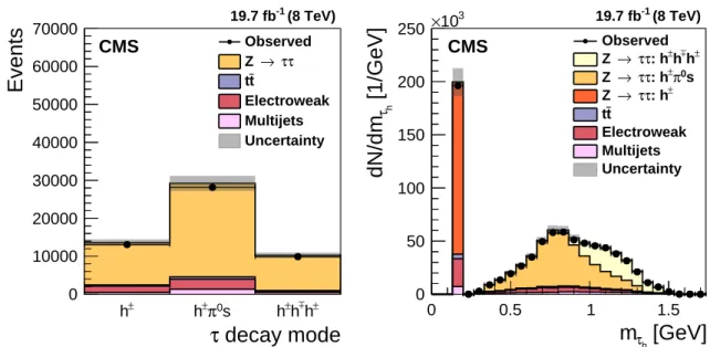
combinations are discarded, resulting in a unique τ_hcandidate to be associated to each jet. The distributions in the decay modes and in the mass of τh candidates in Z/γ∗ → ττ events

are shown in Fig. 3. The contribution of the Z/γ∗ → ττsignal is split according to the recon-structed τhmode, as shown in the legend. For τh candidates reconstructed in the h±π0s and h±h∓h± modes, the mτ_h distribution peaks near the intermediate ρ(770)and a1(1260)meson

resonances (cf. Table 1), as expected. The narrow peak at the charged pion mass is due to τh

candidates reconstructed in the h±mode.

5.2 Tau-isolation discriminants

Requiring reconstructed τ_hcandidates to pass strict isolation requirements constitutes the main handle for reducing the large multijet background. Tau leptons are usually isolated relative to other particles in the event, and so are their decay products, in contrast to quark and gluon jets. Two types of τh isolation discriminants have been developed, using simple cutoff-based

decay mode

τ

Events

[GeV]

m

[1/GeV]

dN/dm

Figure 3: Distributions in (left) reconstructed τ_h decay modes and (right) τ_hcandidate masses in Z/γ∗ → ττevents selected in data, compared to MC expectations. The Z/γ∗ →ττ events are selected in the decay channel of muon and τh, as described in Section 7.1.1. The τh are

required to pass the medium working point of the MVA-based τh isolation discriminant. The

mass of τh candidates reconstructed in simulated Z/γ∗ → ττ events is corrected for small data/MC differences in the τh energy scale, discussed in Section 9. The electroweak

back-ground is dominated by W+jets production, with minor contributions arising from single top quark and diboson production. The shaded uncertainty band represents the sum of systematic and statistical uncertainties on the MC simulation.

selections and an MVA approach. An overview of the discriminants, with their respective efficiencies and misidentification rates, is given in Table 2.

5.2.1 Cutoff-based discriminants

The isolation of τhcandidates is computed by summing the scalar values of pTof charged

par-ticles and photons with pT>0.5 GeV, reconstructed with the PF algorithm, within an isolation

cone of size∆R=0.5, centred on the τhdirection. The effect of pileup is reduced by requiring

the tracks associated to charged particles considered in the isolation sum to be compatible with originating from the production vertex of the τhcandidate within a distance of∆z<0.2 cm and

∆r< 0.03 cm. Charged hadrons used to form the τhcandidate are excluded from the isolation

sum, as are electrons and photons used to construct any of the strips. The effect of pileup on photon isolation is compensated on a statistical basis through the modified∆β corrections:

Iτ =

∑

∑

where the∆β are computed by summing the pT of charged particles that are within a cone of

size∆R=0.8 around the τhdirection, and are associated to tracks that have a distance to the τh

production vertex of more than 0.2 cm in z. The sum is scaled by a factor 0.46, chosen to make the τ_hidentification efficiency insensitive to pileup:

∆β=0.46

∑

charged,∆z>0.2 cm

5.2 Tau-isolation discriminants 11

Loose, medium, and tight working points (WP) are defined for the cutoff-based τh isolation

discriminants by requiring the pT sum defined by Eq. (4) not to exceed thresholds of 2.0, 1.0,

and 0.8 GeV, respectively.

5.2.2 MVA-based discriminants

In order to minimize the jet → τ_h background, the MVA-based τ_h identification discriminant utilizes the transverse impact parameter of the “leading” (highest pT) track of the τhcandidate,

defined as the distance of closest approach in the transverse plane of the track to the τh

pro-duction vertex. It also uses, for τh candidates reconstructed in the h±h∓h± decay mode, the

distance between the τ production point and the decay vertex. A BDT is used to discriminate τhdecays (“signal”) from quark and gluon jets (“background”). The variables used as inputs

to the BDT are:

1. The charged- and neutral-particle isolation sums defined in Eq. (4) as separate inputs. 2. The reconstructed τh decay mode, represented by an integer that takes the value of 0 for

τhcandidates reconstructed in the h±decay mode, as 1 and 2 for candidates reconstructed

in the h±π0and h±π0π0decay modes, respectively, and 10 for candidates reconstructed in the h±h∓h±decay mode.

3. The transverse impact parameter d0of the leading track of the τhcandidate, and its value

divided by its uncertainty, which corresponds to its significance d0/σd0.

4. The distance between the τ production and decay vertices, |~rSV−~rPV|, and its

signifi-cance,|~rSV−~rPV|/σ|~rSV−~rPV|, and a flag indicating whether a decay vertex has successfully

been reconstructed for a given τhcandidate. The positions of the vertices,~rSVand~rPV, are

reconstructed using the adaptive vertex fitter algorithm [48].

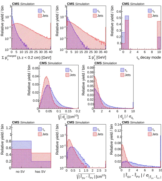
The position of the primary event vertex is refitted after excluding the tracks associated with the τhcandidate. The discrimination power of individual input variables is illustrated in Fig. 4.

The inputs are complemented by the pT and η of the τh candidate and by the ∆β correction

defined in Eqs. (4) and (5). The purpose of the pT and η variables is to parameterize possible

dependences of the other input variables on pT and η. The events used for the training of the

BDT are reweighted such that the two-dimensional pTand η distribution of the τhcandidates

for signal and background are identical, which makes the MVA result independent of event kinematics. The ∆β correction parameterizes the dependence on pileup, in particular, the pT

sum of the neutral particles.

The BDT is trained on event samples produced using MC simulation. Samples of Z/γ∗ → ττ, H → ττ, Z0 → ττ, and W0 → τντ events are used for the “signal” category. Reconstructed τ_hcandidates are required to match τ_hdecays within∆R < 0.3 at the generator level. Multi-jet and W+Multi-jets events are used for the “background” category. The τh candidates that match

leptons originating from the W boson decays are excluded from the training. The samples con-tain ≈ 107 events in total, and cover the range 20–2000 GeV in τh candidate pT. Half of the

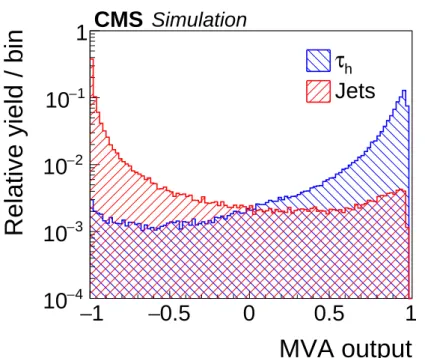
available events are used for training, the other half for evaluating the MVA performance, and conducting overtraining checks. The distribution in MVA output is shown in Fig. 5.

Different working points, corresponding to different τ_h identification efficiencies and jet → τ_h misidentification rates, are defined by changing the selections on the MVA output. The thresholds are adjusted as function of the pT of the τhcandidate, such that the τhidentification

z < 0.2 cm) [GeV] ∆ ( charged T p Σ 0 5 10 15 20 25 30 35 40

Relative yield / bin

4 − 10 3 − 10 2 − 10 1 − 10 1 h τ Jets CMSSimulation [GeV] γ T p Σ 0 5 10 15 20 25 30 35 40

Relative yield / bin

4 − 10 3 − 10 2 − 10 1 − 10 1 h τ Jets CMSSimulation decay mode h τ 0 2 4 6 8 10

Relative yield / bin

0 0.1 0.2 0.3 0.4 0.5 0.6 τh Jets CMSSimulation ] 1/2 [cm | 0 | d 0 0.05 0.1 0.15 0.2

Relative yield / bin

0 0.01 0.02 0.03 0.04 0.05 h τ Jets CMSSimulation 0 d σ | / 0 | d 0 2 4 6 8 10

Relative yield / bin

0 0.01 0.02 0.03 0.04 0.05 0.06 0.07 0.08 0.09 h τ Jets CMSSimulation

Relative yield / bin

0 0.2 0.4 0.6 0.8 1 1.2 no SV has SV h τ Jets CMSSimulation ] 1/2 [cm | PV r - SV r | 0 0.5 1 1.5 2 2.5 3

Relative yield / bin

4 − 10 3 − 10 2 − 10 1 − 10 1 h τ Jets CMSSimulation | PV r - SV r | σ | / PV r - SV r | 0 2 4 6 8 10

Relative yield / bin

0 0.02 0.04 0.06 0.08 0.1 0.12 0.14 h τ Jets CMSSimulation

Figure 4: Distributions, normalized to unity, in observables used as input variables to the MVA-based isolation discriminant, for hadronic τ decays in simulated Z/γ∗ →ττ(blue), and jets in simulated W+jets (red) events. The τhcandidates must have pT >20 GeV and|η| <2.3, and be reconstructed in one of the decay modes h±, h±π0, h±π0π0, or h±h∓h±. In the plot of the τ_h decay mode on the upper right, an entry at 0 represents the decay mode h±, 1 and 2 represent the decay modes h±π0 and h±π0π0, respectively, and entry 10 represents the h±h∓h± decay mode.

5.3 Discriminants against electrons and muons 13

MVA output

1

−

−

0.5

0

0.5

1

Relative yield / bin

4 −

10

10

10

10

1

τ

Jets

CMS

Simulation

Figure 5: Distribution of MVA output for the τh identification discriminant that includes

life-time information for hadronic τ decays in simulated Z/γ∗ → ττ(blue), and jets in simulated W+jets (red) events.

5.3 Discriminants against electrons and muons

Electrons and muons have a sizeable probability to get reconstructed in the h± decay mode. Electrons radiating a bremsstrahlung photon that subsequently converts may also get recon-structed in the h±π0decay mode. In particular, electrons and muons originating from decays of W and Z bosons, which are produced with cross sections of≈100 nb at the LHC at√s=8 TeV, have a high chance to pass isolation-based τh identification criteria. Dedicated discriminants

have been developed to separate τhfrom electrons and muons. The separation of τhfrom

elec-trons is based on an MVA approach. A cutoff-based and an MVA based discriminant are used to separate τhfrom muons.

5.3.1 MVA-based electron discriminant

A BDT discriminant is trained to separate τh decays from electrons. The algorithm utilizes

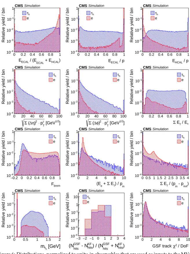
observables that quantify the distribution in energy depositions in the ECAL, in combination with observables sensitive to the amount of bremsstrahlung emitted along the leading track, and observables sensitive to the overall particle multiplicity, to distinguish electromagnetic from hadronic showers. More specifically, the following variables are used as inputs to the BDT:

1. Electromagnetic energy fraction, EECAL/(EECAL+EHCAL), defined as the ratio of energy

depositions in the ECAL to the sum of energy in the ECAL and HCAL, associated with the charged particles and photons that constitute the τhcandidate.

2. EECAL/p and EHCAL/p, defined as ratios of ECAL and HCAL energies relative to the

momentum of the leading charged-particle track of the τhcandidate.

3. q ∑(∆η)2_pγ T and q ∑(∆φ)2_pγ

T, the respective pT-weighted (in GeV) root-mean-square

4. ∑ Eγ/Eτ, the fraction of τhenergy carried by photons.

5. Fbrem = (pin−pout)/pin, where pinand poutare measured by the curvature of the leading

track, reconstructed using the GSF algorithm, at the innermost and outermost positions of the tracker.

6. (Ee+∑ Eγ)/pin, the ratio between the total ECAL energy and the inner track

momen-tum. The quantities Ee and ∑ Eγ represent the energies of the electron cluster and of

bremsstrahlung photons, respectively. ∑ Eγ is reconstructed by summing the energy de-positions in ECAL clusters located along the tangent to the GSF track.

7. _{∑ Eγ}/(pin−pout), the ratio of energies of the bremsstrahlung photons measured in the

ECAL and in the tracker.

8. mτ_h, the mass of the τhcandidate.

9. (NGSF

hits −NhitsKF)/(NhitsGSF+NhitsKF), with NhitsGSFand NhitsKF representing, respectively, the

num-ber of hits in the silicon pixel and strip tracking detector associated with the track recon-structed using, respectively, the GSF and Kalman filter (KF) track reconstruction algo-rithms. The KF algorithm is the standard algorithm for track reconstruction at CMS [21]. The number of hits associated with GSF and KF track is sensitive to the emission of hard bremsstrahlung photons.

10. χ2per degree-of-freedom (DoF) of the GSF track.

The discriminating power of these variables is illustrated in Fig. 6.

The inputs are complemented by the pT and η of the τh candidate, the pT, σpT/pT, and η of

the GSF track, and by the distances in η and in φ of the GSF track to the nearest boundary between ECAL modules. These variables are used to parameterize the dependence of the other input variables. Electrons entering the boundaries between ECAL modules are more difficult to discriminate from τ_hdecays, as their electromagnetic showers are often not well reconstructed, and the probability to reach the hadron calorimeter increases in these regions.

Samples of simulated Z/γ∗ → ττ, Z/γ∗ → ee, W → τντ, W → eνe, tt, H → ττ, Z0 → ττ, Z0 → ee, W0 → τντ, and W0 → eνeevents have been used to train the BDT. Reconstructed τh

candidates are considered as signal or background when they are matched, respectively, within ∆R<0.3 to a hadronic τ decay or to an electron at the generator level.

Different WP are defined by changing the cutoff on the BDT output. The τ_h candidates recon-structed in the uninstrumented region between ECAL barrel and endcap, 1.45< η< 1.56, are rejected in all cases.

5.3.2 Cutoff-based muon discriminant

The cutoff-based discriminant against muons vetoes τh candidates when signals in the muon

system are found near the τ_hdirection. Two working points are provided:

1. Loose: τh candidates pass the cutoff on this discriminant, except when track segments

are found in at least two muon stations within a cone of size∆R =0.3 centred on the τh

direction, or when the sum of the energies in the ECAL and HCAL corresponds to< 0.2 of the momentum of the leading track of the τ_hcandidate.

5.3 Discriminants against electrons and muons 15 ) HCAL + E ECAL / (E ECAL E 0 0.2 0.4 0.6 0.8 1

Relative yield / bin

4 − 10 3 − 10 2 − 10 1 − 10 1 h τ e CMSSimulation / p ECAL E 0 0.2 0.4 0.6 0.8 1

Relative yield / bin

4 − 10 3 − 10 2 − 10 1 − 10 1 h τ e CMSSimulation / p HCAL E 0 0.2 0.4 0.6 0.8 1

Relative yield / bin

4 − 10 3 − 10 2 − 10 1 − 10 1 h τ e CMSSimulation ] 1/2 [GeV γ T p ⋅ 2 ) η ∆ ( Σ 0 20 40 60 80 100

Relative yield / bin

4 − 10 3 − 10 2 − 10 1 − 10 1 h τ e CMSSimulation ] 1/2 [GeV γ T p ⋅ 2 ) φ ∆ ( Σ 0 20 40 60 80 100

Relative yield / bin

4 − 10 3 − 10 2 − 10 1 − 10 1 h τ e CMSSimulation τ / E γ E Σ 0 0.2 0.4 0.6 0.8 1

Relative yield / bin

4 − 10 3 − 10 2 − 10 1 − 10 1 h τ e CMSSimulation brem F 0.2 − 0 0.2 0.4 0.6 0.8 1

Relative yield / bin

4 − 10 3 − 10 2 − 10 1 − 10 1 h τ e CMSSimulation in ) / p γ E Σ + e (E 0 2 4 6 8 10

Relative yield / bin

4 − 10 3 − 10 2 − 10 1 − 10 1 h τ e CMSSimulation ) out - p in / (p γ E Σ 0 0.5 1 1.5 2 2.5 3 3.5 4

Relative yield / bin

4 − 10 3 − 10 2 − 10 1 − 10 1 h τ e CMSSimulation [GeV] h τ m 0 0.5 1 1.5 2

Relative yield / bin

4 − 10 3 − 10 2 − 10 1 − 10 1 h τ e CMSSimulation ) KF hits + N GSF hits ) / (N KF hits - N GSF hits (N 3 − −2 −1 0 1 2 3 4

Relative yield / bin

4 − 10 3 − 10 2 − 10 1 − 10 1 10 τh e CMSSimulation / DoF 2 χ GSF track 0 2 4 6 8 10

Relative yield / bin

4 − 10 3 − 10 2 − 10 1 − 10 1 h τ e CMSSimulation

Figure 6: Distributions, normalized to unity, in observables that are used as inputs to the MVA-based electron discriminant, for hadronic τ decays in simulated Z/γ∗ → ττ (blue), and elec-trons in simulated Z/γ∗ → ee (red) events. The τh candidates must have pT > 20 GeV and |η| <2.3, and be reconstructed in one of the decay modes h±, h±π0, h±π0π0, or h±h∓h±. The rightmost bin of the distributions is used as overflow bin.

2. Tight: τhcandidates pass this discriminant restriction when they pass the loose WP, and

no hits are present within a cone of∆R=0.3 around the τhdirection in the CSC, DT, and

RPC detectors located in the two outermost muon stations. 5.3.3 MVA-based muon discriminant

A multivariate BDT discriminant has also been trained to separate τhdecays from muons. The

following variables are used as BDT inputs:

1. The calorimeter energy associated with the leading charged particle of the τhcandidate,

with separate energy sums computed for ECAL and HCAL.

2. The calorimeter energy associated in the PF algorithm with any charged particle or pho-ton constituting the τhcandidate, again, with separate energy sums computed for ECAL

and HCAL.

3. The fraction of pT carried by the charged particle with highest pT.

4. The number of track segments in the muon system reconstructed within a cone of size ∆R=0.5 around the τhdirection.

5. The number of muon stations with at least one hit detected within a cone of size∆R=0.5 centred on the τhdirection, computed separately for DT, CSC, and RPC detectors.

The inputs are complemented by the η of the τh candidate, to parameterize the dependence

of the input variables on the DT, CSC, and RPC muon acceptance, and on the path length of muons traversed in the ECAL and HCAL.

The BDT is trained using samples of simulated Z/γ∗ →ττ, Z/γ∗ → µµ, W→τντ, W→µνµ, tt, H→ττ, Z0 →ττ, Z0 →µµ, W0 →τντ, and W0 →µνµevents. Reconstructed τhcandidates

are considered as signal or background when they are matched, respectively, to generator-level hadronic tau decays or muons within∆R<0.3.

Different WP are defined by changing the cutoff on the MVA output.

6

Expected performance

The expected performance of the HPS τ_hidentification algorithm is studied in terms of decay modes and energy reconstruction, τh identification efficiency, and misidentification rates for

jets, electrons, and muons using simulated samples of Z/γ∗ → `` (` = e, µ, τ), Z0 → ττ, W+jets, and multijet events.

Tau identification efficiencies and misidentification rates in MC simulated events, averaged over pT and η, for pileup conditions characteristic of the data-taking period, are given in

Ta-ble 2.

6.1 Decay modes and energy reconstruction

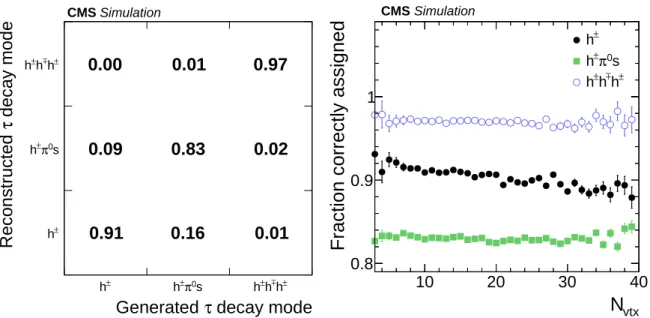
The τ_hdecay mode reconstruction is studied in simulated Z/γ∗ →ττevents. The performance is quantified by the correlation between reconstructed and generator-level τ_h decay modes. Figure 7 demonstrates that the true τ decay mode is reconstructed in about 90% of the cases, irrespective of pileup conditions, represented by the number of reconstructed vertices (Nvtx).

6.1 Decay modes and energy reconstruction 17

Table 2: Expected efficiencies and misidentification rates of various τ_h identification discrim-inants, averaged over pT and η, for pileup conditions characteristic of the LHC Run 1

data-taking period. The DM-finding criterion refers to the requirement that the τh candidate be

reconstructed in one of the decay modes h±, h±π0, h±π0π0, or h±h∓h±(cf. Section 5.1). DM-finding and τhisolation discriminants

WP Efficiency Jet→τhmisidentification rate

Z/γ∗ →ττ Z0(2.5 TeV) →ττ W+jets Multijet

Cutoff-based Loose 49.0% 58.9% 9.09×10−3 _3.86×10−3 Medium 40.8% 50.8% 5.13×10−3 _2.06×10−3 Tight 38.1% 48.1% 4.38×10−3 1.75×10−3 MVA-based Very loose 55.9% 71.2% 1.29×10−2 6.21×10−3 Loose 50.7% 64.3% 7.38×10−3 3.21×10−3 Medium 39.6% 50.7% 3.32×10−3 _1.30×10−3 Tight 27.3% 36.4% 1.56×10−3 4.43×10−4

Discriminant against electrons

WP Efficiency e→τhmisidentification rate

Z/γ∗→ττ Z0(2.5 TeV) →ττ Z/γ∗→ee Very loose 94.3% 89.6% 2.38×10−2 Loose 90.6% 81.5% 4.43×10−3 Medium 84.8% 73.2% 1.38×10−3 Tight 78.3% 65.1% 6.21×10−4 Very tight 72.1% 60.0% 3.54×10−4

Discriminant against muons

WP Efficiency µ→τhmisidentification rate

Z/γ∗ →ττ Z0(2.5 TeV) →ττ Z/γ∗ →µµ Cutoff-based Loose 99.3% 96.4% 1.77×10−3 Tight 99.1% 95.0% 7.74×10−4 MVA-based Loose 99.5% 99.4% 5.20×10−4 Medium 99.0% 98.8% 3.67×10−4 Tight 98.0% 97.7% 3.18×10−4

are reconstructed in the true decay mode is due to events in which particles from pileup deposit energy in the ECAL near the τ, causing the τ to be reconstructed in the h±π0or h±π0π0decay modes.

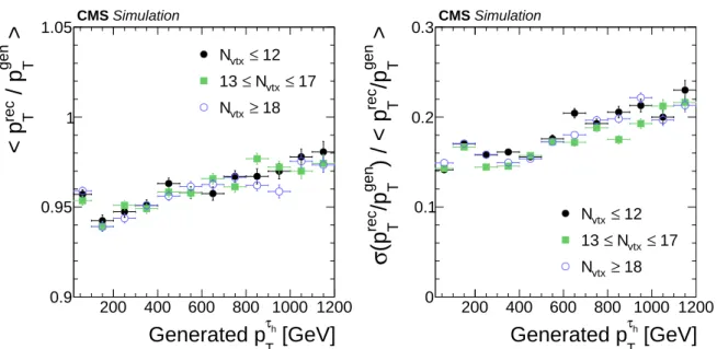
The performance of energy reconstruction is studied in simulated Z/γ∗ → ττ and Z0 → ττ events, and quantified in terms of response and resolution, defined as the mean and standard deviation of the reconstructed momentum distribution relative to the generator-level momen-tum of the visible τ decay products. The distributions for τhdecays in simulated Z/γ∗ → ττ and Z0 → ττ events are shown in Fig. 8. The average response is below 1.0, because of an asymmetry of thehprec_T /pgen_T idistribution, where prec_T and pgen_T refer, respectively, to the pT of

the reconstructed τ_h candidate and to the pT of the vectorial momentum sum of the visible τ

decay products at the generator level. The most probable value of the ratiohprec

T /p

gen

T iis close

to 1.0. The effect of pileup on τ reconstruction is small.

0.91 0.16 0.01 0.09 0.83 0.02 0.00 0.01 0.97 decay mode τ Generated ± h _h±π0s _h±_hh± ± decay mode τ Reconstructed ± h s 0 π ± h ± h ± h ± h CMS Simulation vtx

N

Fraction correctly assigned

0.8 0.9 1 ± h s 0 π ± h ± h ± h ± h CMS Simulation

Figure 7: Left: Correlation between generated and reconstructed τhdecay modes for τhdecays

in Z/γ∗ → ττ events, simulated for pileup conditions characteristic of the LHC Run 1 data-taking period. Right: Fraction of generated τh reconstructed in the correct decay mode as

function of Nvtx. Reconstructed τhcandidates are required to be matched to hadronic τ decays

at the generator-level within∆R<0.3, to be reconstructed in one of the decay modes h±, h±π0, h±π0π0, or h±h∓h±, and pass pT >20 GeV,|η| < 2.3, and the loose WP of the cutoff-based τ_h isolation discriminant.

6.2 The τh identification efficiency

The efficiency to pass the decay mode reconstruction and the different τh identification

dis-criminants is determined for hadronic τ decays with visible decay products that satisfy the conditions pT >20 GeV and|η| < 2.3 at the generator level. More specifically, the efficiency is defined by the percentage of τ_hcandidates that satisfy:

ετ =

prec_T >20 GeV,|ηrec| <2.3, DM-finding, τhID discriminant

pgen_T >20 GeV, |ηgen| <2.3

, (6)

where ηrecand ηgen refer, respectively, to the η of the reconstructed τh candidate and to the η

of the vectorial momentum sum of the visible τ decay products at the generator level. The DM-finding criterion refers to the requirement that the τh candidate be reconstructed in one

6.2 The τhidentification efficiency 19

[GeV]

Generated p

>

/ p

< p

[GeV]

Generated p

>

/p

) / < p

/p

(p

σ

Figure 8: The τ_henergy response (left) and relative resolution (right) as function of generator-level visible τ pT in simulated Z0 → ττ events for different pileup conditions: Nvtx ≤ 12,

13 ≤ Nvtx ≤ 17, and Nvtx ≥ 18. Reconstructed τh candidates are required to be matched to

hadronic τ decays at the generator-level within ∆R < 0.3, to be reconstructed in one of the decay modes h±, h±π0, h±π0π0or h±h∓h±, and to pass pT > 20 GeV,|η| <2.3, and the loose WP of the cutoff-based τhisolation discriminant.

of the decay modes h±, h±π0, h±π0π0, or h±h∓h± (cf. Section 5.1), and τ_h ID refers to the τ_h identification discriminant used in the analysis. The pgen_T and ηgen selection criteria in the

denominator are also applied in the numerator. Only those τhcandidates matched to

generator-level hadronic τ decays within∆R<0.3 are considered in the numerator.

The efficiencies of the discriminants against electrons and muons are determined for τh

candi-dates matched to generator-level τhdecays within∆R<0.3, passing prec_T >20 GeV,|ηrec| <2.3,

reconstructed in one of the decay modes h±, h±π0, h±π0π0, or h±h∓h±, and satisfying the loose WP of the cutoff-based τ_hisolation discriminant:

ετ =

lepton discriminant

prec_T >20 GeV, |ηrec| <2.3, DM-finding, loose cutoff-based isolation. (7)

The selection criteria in the denominators of Eqs. (6) and (7) are also applied in the numerators. The efficiency for τ_hdecays to pass the cutoff-based and MVA-based τ_hidentification discrim-inants are shown for simulated Z/γ∗ →ττand Z0 →ττevents in Fig. 9.

The efficiencies are higher in Z0 → ττ than in SM Z/γ∗ → ττ events, as the τ leptons have larger pT in the former case. The expected efficiencies of the isolation discriminants range

between 40% and 70%, depending on whether tight or loose criteria are applied. The discrimi-nation against electrons and against muons have respective efficiencies between 60% and 95%, and between 95% and 99%.

[GeV]

Generated p

efficiency

τ

Expected

1.2 Loose cutoff-based isolation Medium cutoff-based isolation Tight cutoff-based isolation CMS Simulation τ τ → * γ Z/

[GeV]

Generated p

efficiency

τ

Expected

1.2 Loose cutoff-based isolation Medium cutoff-based isolation Tight cutoff-based isolation CMS Simulation τ τ → Z' (2.5 TeV)

[GeV]

Generated p

efficiency

τ

Expected

1.2 Very loose MVA isolation

Loose MVA isolation Medium MVA isolation Tight MVA isolation CMS Simulation τ τ → * γ Z/

[GeV]

Generated p

efficiency

τ

Expected

1.2 Very loose MVA isolation

Loose MVA isolation Medium MVA isolation Tight MVA isolation CMS Simulation

τ τ →

Z' (2.5 TeV)

Figure 9: Efficiency for τ_h decays in simulated Z/γ∗ → ττ (left) and Z0 → ττ (right) events to be reconstructed in one of the decay modes h±, h±π0, h±π0π0, or h±h∓h±, to satisfy the conditions pT > 20 GeV and |η| < 2.3, and to pass: the loose, medium and tight WP of the

cutoff-based τhisolation discriminant (top) and the very loose, loose, medium and tight WP of

the MVA-based tau isolation discriminant (bottom). The efficiency is shown as a function of the generator-level pTof the visible τ decay products in τhdecays that are within|η| <2.3.

6.3 Misidentification rate for jets 21

6.3 Misidentification rate for jets

The rate at which quark and gluon jets are reconstructed as τhcandidates passing τ

identifica-tion is computed for jets with pjet_T >20 GeV and|ηjet| <2.3 as follows:

P_misid = p

τh

T >20 GeV, |ητh| <2.3, DM-finding, τhID discriminant

pjet_T >20 GeV,|ηjet| <2.3

. (8)

The pjet_T and ηjet selection criteria of the denominator are also applied in the numerator. Note

that pT and η are different in the numerator and denominator, because pjet_T and ηjet are

com-puted by summing the momenta of all the particle constituents of the jet, while pτh

T and ητh

refer to only the charged particles and photons included in the decay mode reconstruction of the τhcandidate. Besides, jet energies are calibrated [51] and corrected for pileup effects [52, 53],

whereas no energy calibration or pileup correction is applied to τhcandidates.

The rates of jet→τhmisidentification range from a few 10−4to 10−2. They differ for W+jets and

multijet events, because of the different fractions of quark and gluon jets in the two samples, and because of differences in jet pTspectra, which are relevant due to the dependence of the jet →τ_hmisidentification rates on jet pT(cf. Section 10).

The MVA-based τhidentification discriminants that include lifetime information reduce the jet → τhmisidentification rate by about 40% relative to cutoff-based discriminants, while the τh

identification efficiencies are very similar.

6.4 Misidentification rate for electrons and muons

The misidentification rates for e → τh and µ → τh are determined for electrons and muons

with p`<sub>T</sub> >20 GeV and|η`| <2.3, and can be written as follows:

Pmisid=

pτh

T >20 GeV,|ητh|,<2.3, DM-finding, loose cutoff-based isolation, lepton discriminant

p`

T >20 GeV, |η`| <2.3

. (9) Only τh candidates reconstructed within ∆R < 0.3 of a generator-level electron or muon

tra-jectory are considered for the numerator. The p`<sub>T</sub>and η` symbols refer to the generator-level pT

and η of the electron or muon.

Typical e → τh misidentification rates range from a few per mille to a few per cent. The rates

for µ→τhmisidentification are at or below the per mille level.

7

Validation with data

Different kinds of events are used to evaluate the τh reconstruction and identification in data.

The τh identification efficiency and energy scale are validated using Z/γ∗ → ττ events. The

efficiency to reconstruct and identify τh of higher pT in more dense hadronic environments is

measured using tt events. Samples of W+jets and multijet events are used to validate the rates with which quark and gluon jets are misidentified as τhcandidates. The misidentification rates

for electrons and muons are measured using Z/γ∗ →ee and Z/γ∗ →µµevents.

The selection of event samples is described in Section 7.1. Systematic uncertainties relevant to the validation of the τh reconstruction and identification are detailed in Section 7.2. The

measurement of τhidentification efficiency, as well as of the rates at which electrons and muons

processes, for which we use fits of simulated distributions (templates) to data, as described in Section 7.3.

7.1 Event selection 7.1.1 Z/γ∗→ττ events

The sample of Z/γ∗ → ττ events is selected in decay channels of τ leptons to muon and τh

final states. Except for extracting the τhidentification efficiency, Z/γ∗ →ττ → µτhevents are

recorded using a trigger that demands the presence of a muon and τ_h[9]. The events used for the τ_h identification efficiency measurement are recorded using a single-muon trigger [46], to avoid potential bias that may arise from requiring a τh at the trigger level. The reconstructed

muon is required to satisfy the conditions pT>20 GeV and|η| <2.1, to pass tight identification

criteria, and to be isolated relative to other particles in the event by Iµ < 0.10pµ_T, computed according to Eq. (1). The τh candidates are required to be reconstructed in one of the decay

modes described in Section 5.1, to satisfy the conditions pT >20 GeV and|η| <2.3, and to pass the loose WP of the cutoff-based τh isolation discriminant, the tight WP of the cutoff-based

discriminant against muons, and the loose WP of the discriminant against electrons. The muon and τ_h candidate are required to be compatible with originating from the primary collision vertex and be of opposite charge. In case multiple combinations of muon and τ_h exist in an event, the combination with the highest sum in scalar pT is chosen. Background arising from

W+jets production is removed by requiring the transverse mass computed in Eq. (3) to satisfy the condition mT <40 GeV. Events containing a second muon of pT > 15 GeV and|ηµ| < 2.4, passing loose identification and isolation criteria, are rejected to suppress Z/γ∗ → µµ Drell– Yan (DY) background.

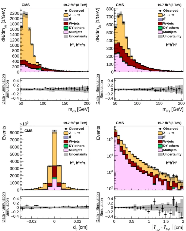
The transverse impact parameter d0and the distance|~rSV−~rPV|between the τ production and

decay vertices in selected Z/γ∗ → ττ events are shown in Fig. 10. The normalization of the Z/γ∗ → ττ → µτ_h signal and of background processes is determined through a template fit to the data, as described in Section 7.3, using the visible mass of the muon and τh (mvis) as

observable in the fit. Separate fits are performed for events with τhcandidates containing one

and three charged particles. The fitted mvisspectra are also shown in Fig. 10. The shaded areas

represent the sum of statistical uncertainties of the MC samples and systematic uncertainties, added in quadrature, as discussed in Section 7.2. All distributions agree well with their respec-tive MC simulations.

7.1.2 tt events

A sample of tt events is also selected in the µτhchannel. The tt→bbµτhevents are required to

pass a single-muon trigger and to contain a muon with pT >25 GeV and|η| < 2.1. The muon is required to pass tight identification criteria and to be isolated at the level of Iµ <0.10p

µ

T. The τ_hcandidate is required to be reconstructed in one of the decay modes described in Section 5.1, to satisfy the conditions pT > 20 GeV and|η| < 2.3, to pass the loose WP of the cutoff-based τ_hisolation discriminant, and to be separated from the muon by ∆R > 0.5. The event is also required to contain two jets of pT >30 GeV and|η| <2.5, separated from the muon and the τh

candidate by∆R>0.5. At least one of the jets is required to meet the b tagging criteria [54, 55]. Background from Z/γ∗ → `` (` = e, µ, τ) events is reduced by requiring Emiss_T > 40 GeV. Events containing an electron of pT >15 GeV and|η| < 2.3, or a second muon of pT >10 GeV

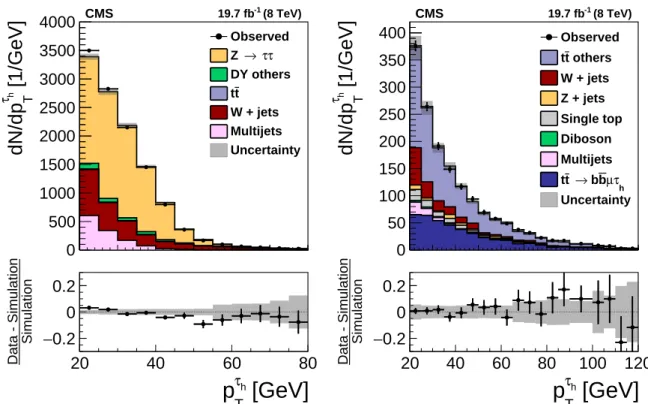
and|η| <2.4 that pass loose identification and isolation criteria are rejected.

The pT distribution of τhcandidates in the tt sample is compared to the Z/γ∗ → ττsample in