Quantitative analysis of Bicyclus anynana's eyespot wing pattern images

Texto

(1)Universidade de Lisboa Faculdade de Ciências Departamento de Biologia Animal . QUANTITATIVE ANALYSIS OF BICYCLUS ANYNANA‘S EYESPOT WING PATTERN IMAGES Pedro dos Santos Lopes Mestrado em Bioinformática e Biologia Computacional, 2011 Bioinformática . . . .

(2) . . .

(3) Universidade de Lisboa Faculdade de Ciências Departamento de Biologia Animal . QUANTITATIVE ANALYSIS OF BICYCLUS ANYNANA‘S EYESPOT WING PATTERN IMAGES Pedro dos Santos Lopes Mestrado em Bioinformática e Biologia Computacional, 2011 Bioinformática . Master dissertation supervised by Dra. Filipa Alves, Instituto Gulbenkian de Ciência Dr. Gabriel G Martins, Faculdade de Ciências da Universidade de Lisboa. .

(4) Index Abstract ................................................................................... i Resumo ................................................................................. iii Introduction ........................................................................... 1 Objectives............................................................................... 3 Implementation ..................................................................... 4 Input dialog ................................................................................. 5 Separation of each eyespot (wing) ............................................ 10 Analysis of the eyespot ............................................................. 14 Analysis of normal images ............................................................ 14 Analysis of fluorescent microscopy images .................................. 23 . Auxiliary methods ..................................................................... 26 . Results .................................................................................. 27 Discussion ............................................................................. 39 Initial approach ......................................................................... 40 Current approach ...................................................................... 42 Future developments ................................................................ 46 . References ............................................................................ 47 Annexes ................................................................................ 49 Variables .................................................................................... 49 . . . .

(5) . .

(6) Abstract The main objective of this work is to provide researchers with a tool to quantitatively analyse images of the eyespot patterns present in the wings of the butterfly species Bicyclus anynana. More specifically, this tool is a plugin for imageJ, a free open‐sourced image processing program. Until now, researchers have been using software such as imageJ to quantify some dimensions of these patterns through manual measurements. This plugin offers an effective, quick and automatic way to obtain these measurements and others more difficult to get until now, such as the area of each coloured region. It also offers the possibility to obtain representative images of the eyespot(s). Besides images with a single eyespot, the program also analyses wing images with several eyespots as well as fluorescence microscopy images with specific proteins labelled. In the first two types, the program finds the eyespots automatically and analyses them individually, and in the latter ones, the program can provide us with intensity plots of transversal cuts through the middle of the eyespot. To obtain the required data, the plugin finds the centre of each eyespot and, from there, searches for the frontiers of each of its coloured areas. It then calculates their area, diameter and roundness which will be used to calculate the rest of the needed data and to create the representative images. In case of fluorescence microscopy images, the program unites its coloured dots through a dilation process and then acquires the intensity plots. In the end, we have a program that gives more and better data to help future research on evolution and development using this species and that could subsequently be transformed into a more generic plugin capable of analysing any pattern containing closed frontiers due to its strong aptitude to obtain these, regardless of any possible background noise. Keywords: Bicyclus anynana, ImageJ, eyespots, quantitative analysis, fluorescence microscopy. . i .

(7) Acknowledgements Dra. Filipa Alves, Instituto Gulbenkian de Ciência Dr. Gabriel Martins, Faculdade de Ciências da Universidade de Lisboa . . ii .

(8) . Resumo Este trabalho tem como objectivo proporcionar aos investigadores uma ferramenta para análise quantitativa de padrões eyespot em imagens de asas de borboletas Bicyclus anynana, nomeadamente um plugin para o imageJ, um programa de análise de imagem gratuito open source. Até então tem‐se recorrido ao uso de softwares como o imageJ para obter algumas dimensões destes padrões através de medidores manuais de distâncias que se encontram disponíveis nos ditos softwares. Este plugin oferece um modo rápido e eficaz de obter essas medições de distâncias e outras que até então não eram possíveis de serem obtidas por métodos manuais, como a área de cada região do eyespot e a circularidade (roundness) do mesmo. O plugin também oferece a possibilidade da criação automática de imagens representativas do eyespot em análise, quer usando as fronteiras reais de cada área quer usando representações elípticas das mesmas. Para além de imagens com um eyespot individual, o programa também analisa imagens de asas com vários eyespots bem como imagens de microscopia de fluorescência mostrando expressão da proteina Distal‐less ou Engrailed. Para os primeiros tipos de imagem, o programa encontra automaticamente os eyespots e analisa‐os individualmente, e para os últimos o programa possibilita o retorno de cortes transversais, passando pelo meio do eyespot, através de gráficos de intensidades, que auxiliam o investigador na sua análise. A espécie Bicyclus anynana tem eyespots anterior e posterior nas superficies ventral e dorsal das asas dianteiras e vários eyespots na superficie dorsal das asas traseiras. Estes padrões são circulares e são de diferentes tamanhos e têm a mesma constituição: uma pequena área branca no centro com aproximadamente um centésimo do tamanho do eyespot, uma área preta predominante e uma faixa amarela em torno desta, envolvendo o eyespot. Estes aspectos morfológicos têm uma grande variação genética e todos eles mostraram que reagem em conjunto à selecção artificial e até mesmo a mutações. Esta aparente união é devido a partilharem o mesmo tipo de desenvolvimento, a partir de centros organizadores denominados por foci, sendo também observado uma expressão de genes de desenvolvimento característica em préadultos. No entanto, um grande potencial para variação independente do tamanho do eyespot tem‐se observado. Para estudar mais a fundo estas variações neste tipo de padrão, é preciso obter‐se dados de aspecto mais quantitativo para se ter uma correspondência mais precisa e significativa entre a expressão genética e a variação fenotípica que se observa no indivíduo adulto. Para a obtenção dos dados pretendidos, o plugin, para imagens de eyespots individuais ou imagens de uma asa, obtém o centro do(s) eyespot(s) e, a partir dele, procura as três fronteiras que o constituem. Ao encontrar cada fronteira, o programa regista essas fronteiras individuais e utiliza‐as para obter informações como as áreas, diâmetros e circularidade que depois servem para os cálculos pretendidos de proporções entre áreas ou iii .

(9) criação das imagens representativas. Para a obtenção destas fronteiras, o programa binariza a imagem, onde depois é aplicada a função outline e skeletonize, obtendo‐se assim linhas de um pixel de largura. Depois o programa segue por cada uma delas num determinado sentido e percorre‐as somente pelo caminho mais curto, sem se enganar por possíveis erros presentes na imagem. Para saber qual o caminho a seguir, o programa pinta cada lado de cada linha com uma determinada cor e, para ser a linha correcta, esta tem de ter pelo menos um pixel de cada uma destas cores presente na sua vizinhança. Existem casos especiais que podem ocorrer, como haver mais que um pixel para seguir que contenha as condições certas ou o lado exterior não ter sido completamente pintado para poder seguir em frente, por exemplo. Para estes casos e outros, existem outro tipo de subregras que depois são aplicadas, de modo a possibilitar ao programa seguir em frente e continuar pelo caminho certo. São estas correcções e subregras que fazem com que o plugin seja relativamente robusto em relação a possíveis indefinições existentes na própria imagem. No caso de imagens de uma asa, para se obter dados correctos e individuais para cada eyespot, o programa tem de os separar, e fá‐lo traçando rectas entre eles, de modo a que quando o programa obtém a última fronteira, a exterior, o programa não siga para o eyespot vizinho e o contabilize para os dados do eyespot a ser analisado. Ao finalizar a análise de cada um dos eyespots, o programa volta a pintar o que coloriu com as cores originais, branco para as áreas e preto para as fronteiras, de modo a não ocorrer erros com a análise do eyespot anterior. No caso de imagens de microscopia de fluorescência, sendo esta constituída por pontos coloridos num fundo preto que correspondem à expressão de uma determinada proteína, o programa une esses pontos através de um processo de dilatação para dar volume ao eyespot e proceder então aos cortes transversais pretendidos pelo utilizador. Um dos tipos de cortes possíveis é um corte médio que corresponde a uma média de vários cortes ao longo do eyespot em diferentes ângulos. Para tal, o programa cria uma imagem que é a média entre várias imagens, cada uma delas com uma determinada rotação em relação à anterior com centro no meio da região central do eyespot. O programa também possibilita a obtenção de outros dados como a área, o diâmetro e a circularidade (roundness) para cada região. Como resultado final, tem‐se um programa que analisa quantitativamente os padrões eyespot presente nas asas de borboleta da espécie Bicyclus anynana, que nos possibilita ter uma coneccção mais fidedigna entre o padrão observado e a expressão genética envolvente na sua formação, obtendo‐se assim mais e melhores dados de análise para futuros trabalhos de investigação em evolução e desenvolvimento usando esta espécie. Posteriormente, este plugin pode ser transformado num mais genérico, capaz de analisar qualquer padrão constituido por fronteiras circulares fechadas, devido à sua forte capacidade de obtenção deste tipo de fronteiras apesar de qualquer possível ruido de fundo na imagem. . iv .

(10) Palavras chave: Bicyclus anynana, imageJ, eyespots, análise quantitativa, microscopia de fluorescência. . v .

(11) . . vi .

(12) Introduction The colour patterns on butterfly wings are a great example of phenotypic variation. . These patterns can vary both across and within species and are ecologically significant, often having a known adaptive value. The butterfly Byciclus anynana became an important model to study adaptive morphological evolution in evolutionary developmental biology due to its variable wing color patterns, namely the eyespots, and because it can be easily maintained in the laboratory. Evolutionary and developmental biology is confronted with the task of understanding the genetic bases of phenotypic variation. For this reason, the genetic pathways involved in eyespot formation and the physiological basis of its plasticity as well as the biochemical pathways of the pigments formation have been the object of study (3). Knowledge from Drosophila melanogaster wing development studies have contributed to the understanding of butterfly wing pattern formation, having a number of its developmental pathways been implicated in butterflies, like the Distal‐less (Dll), engrailed (en), spalt (sal) and Notch (N) genes that are expressed in the eyespot area in developing wings. Although useful, this approach only gives us candidate genes from the Drosophila and not all the ones involved in butterfly wing formation (1). Since Diptera and Lepidoptera are quite different, namely, for the case in study, their wings, we can conclude that it is likely that not all the involved genes will be the same as in Drosophila, and a more profound search is necessary to fully understand the butterfly wing colour evolution and development (3). Bicyclus anynana has an anterior and a posterior eyespot on both the dorsal and ventral forewing surfaces and several eyespots on the dorsal hindwing surfaces. Each eyespot is approximatelly circular in shape and may have a different size, but all have the same colour composition: a small white centre area roughly 1/100th of the eyespot, a large middle black area and a narrow yellow ring surrounding it. These morphological aspects have a great phenotypic variation, but all of the eyespots have been shown to react to artificial selection in unison and can also be affected as a group in some wing pattern mutants. This association between the eyespots is due to the fact that they all share the same developmental basis while they are formed from central organizers called foci. The characteristic eyespot shape can already be recognized in the wing disk of the late pupa by the expression pattern of some developmental genes (e.g. en, sal Dll). Consequently, we can view the whole pattern of eyespots as a single module that is evolutionary and developmentally independent from those of other pattern elements present on the wings. Some aspects of eyespot morphology have genetic correspondences between eyespots, being stronger for eyespots on the same wing surface. It has been shown that these correspondences determine the eyespot size and the whole pattern, including in different wing surfaces and, to some degree, other features of eyespot morphology. However, great potential has been found for independent variation of eyespot size even though there’s a strong genetic connection between eyespots on the same wing surface. This goes against 1 .

(13) the prevalent role of developmental constraints derived from the coupling between individual eyespots in shaping the evolution in eyespot size. This seemingly overridden aspect suggests that the genetic correlations aren’t a major factor constraining wing pattern formation. Even though there’s obvious genetic connections, it is known that eyespots from dorsal and ventral surfaces are rather independent, as, for example, the ventral eyespots show plasticity in their size depending on temperature and hormonal regulation whereas dorsal eyespots do not (2). Some genetic tools are currently being developed for B. anynana like the construction of a Bacterial Artificial Chromosome library (3), and an extensive Expression Sequence Tags project is being done, that will help identify new genes involved in wing pattern formation and variation as well as to serve as a basis for the development of a linkage map and DNA microarrays and to help identify DNA sequence polymorphisms in wing genes using its redundancy. These polymorphisms could be then used to build a high‐ density gene‐based linkage map for this species that will be an essential help to the mapping of the wing pattern variation to gene regions, and at the same time testing the contribution of a number of candidate loci to this variation (1). The development of germline transformation techniques for this butterfly is also a recent development in its studies, being the only butterfly species to date where this is possible. All these techniques and tools in development are going to be crucial in testing the function of candidate genes and their contribution to pattern development and evolution, as well as in providing the first steps of the development of more sophisticated gene manipulation techniques already available in other model systems (3). Furthermore, a modelling approach of the pathways involved in the eyespot pattern formation is currently underway in order to help understanding the regulatory relations among the candidate genes, and also to predict other unknown genes possibly involved in this development process. To help this approach, new ways of measuring the eyespots and their phenotypic variation are needed in order to quantify the natural variation in the patterns, as well as the possible experimentally induced alterations, either by artificial selection (selective breeding) or by mutations. To this day, these measurements were made coarsely and prone to human errors as they were being made “by hand”. In order to obtain more precise values, and others that until now weren’t possible to obtain, a new automatic measurement tool must be created and that’s the main goal of this work. By providing a precise quantification of the eyespot images, this tool enables the objective comparison between the different variants of the same pattern, both in wild type and mutant butterflies, thus contributing to stablish a more meaningful correspondence between gene expression and phenotypic variation. . . . 2 .

(14) Objectives The main goal of this work is to provide the researchers working with the butterfly species Bicyclus anynana with a tool to quantitatively analyse images of the eyespots present on their wings. Because the study of their formation cannot be done without studying gene expression, this tool also analyses fluorescence microscopy images of the eyespots where the expression pattern of some genes is analysed. This project uses ImageJ as the platform for the tool created, in this case a plugin. Because it’s a public domain, java‐based image processing program and its source code is freely available, it proved to be a good choice to provide the researchers an inexpensive tool for their works (15). This plugin analyses several different types of images: images with a single cut‐out eyespot on them, images of the whole wing, both fore and hind wings, and fluorescence microscopy images with a single eyespot, showing the homologues of Drosophila melanogaster gene product expression for Engrailed. Previously, the methods used to compare eyespots were rudimentary, such as measuring their diameters with a program ruler, from edge to edge. These types of methods are more laborious and less producible or thorough so a more precise tool is required, one that would automatically identify spots and calculate data such as areas, roundness, diameters, intensities, without the normal human errors and biases that come with manual measurements. This plugin will allow future works on this subject to have more accurate quantitative data rather than manual measurements and comparison of different eyespots, as well as a faster and quicker method/tool to analyse the images collected experimentally. . . . 3 .

(15) Implementation The plugin is composed of four parts as shown in the diagram below. First we have a section that contains the code for creating the initial input dialog in which the user can choose the wanted output parameters, then we have the main body of the program that contains a section to separate each eyespot in case the user analyses the whole wing and a section that performs the analysis of the eyespot. This is the main section which is used to analyse all image types and is divided into two distinct subsections: the first analyses normal images and the other performs the analysis of fluorescence microscopy images. At the end of the code there are some auxiliary methods to be used on the main body. The images used to test and obtain the data to perform comparisons between them comes from the articles referenced at the end after the discussion section. . . Figure 1: main structure of the program. . . . . 4 .

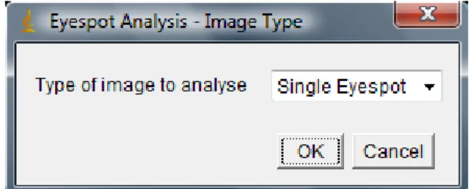
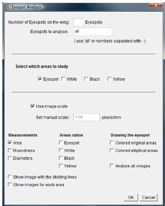
(16) Input dialog The input dialog section contains the code to create the initial menu for the user to choose the output parameters. This initial section actually consists of two separate dialogs: the first one asks the user to select the type of image to be analysed, which is going to define the composition of the next one, and the second will ask the user to choose the output parameters as well as other information, depending on the type of image selected. The first dialog is a very straight forward drop down choicer, as it can be observed on the image below. The user is allowed to choose between “Single Eyespot”, “Forewing”, “Hindwing”, “Distal‐less” and “Engrailed”. . Figure 2: first input dialog for choosing the type of image to analyse. . The program then sets the default number of eyespots in the image, one for “Single Eyespot”, “Distal‐less” and “Engrailed” images, two for “Forewing” images and seven for “Hindwing” images. The second dialog is different for each type of image to analyse. When the user chooses the “Single Eyespot” option, the program will recognize the image as being a normal image (not a fluorescence microscopy one) with a single eyespot cut from a wing, and will analyse it using only the subsection ‘analysis of normal images’. Its second dialog (fig. 3) has two parts: one in which the user selects which areas to study (the options are the eyespot in its totality and each individual areas) and another in which the user can introduce the scale of the image (pixels/mm), manually or selecting the image scale set on imageJ or present in its metadata, and select which output data to get. In the later part, the user can choose to obtain the area, the roundness and the diameters (minimum and maximum) for the selected areas to study. It is also possible to get several areas ratios by selecting which areas to use, as well as image representations of the eyespot using the real frontiers for each area (Coloured original areas) and using elliptical representations of each frontier to draw the eyespot (Coloured elliptical areas). The user can also choose to analyse all the opened images (though they all have to be of the same image type) and to show binary images for each individual area (white, black and yellow). . 5 .

(17) Figure 3: second input dialog for “Single Eyespot” image. . If the user chooses either the “Forewing” or “Hindwing” options, the program will recognize the image as being a normal image of a whole wing (at least with all the eyespots visible) and will analyse it using the ‘separation of each eyespot (wing)’ section and the same analysis used for the previous case. In this case, the second dialog (fig. 4) is the same as the previous one (fig. 3) with an additional part in which the user has to introduce the number of eyespots on the wing as well as which eyespots to analyse, using in this case the word ‘all’ for analyse all eyespots or introducing the number of the eyespots (ordered from top to bottom) separated by a dash (‐). The user can also choose to view the outlined binarized image with the dividing lines (that mimics the division provided by the veins). . 6 .

(18) Figure 4: second input dialog for “Forewing” and “Hindwing” image. . The last two options will tell the program that the image is a fluorescence microscopy one with a single eyespot and will analyse it using only the subsection ‘analysis of fluorescence microscopy images’. The second dialog (fig. 5) is somewhat simpler than the previous ones since it only has the part where the user introduces the scale (pixels/mm), manually or selecting the image scale set on imageJ or present in its metadata, and select which output data to get, such as the area, roundness and diameters (minimum and maximum) for all areas. It is possible to obtain an image representation of the eyespot using elliptical representations of each frontier and cross sections (average, along the minimum diameter and along the maximum diameter), perpendicular to the image. There is also the choice to analyse all the opened images. . 7 .

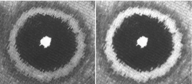
(19) Figure 5: second dialog for the “Distal‐less” and “Engrailed” image. . In order to proceed correctly to the analysis, the program searches the user input for errors and gives the corresponding alert. Some conditions must be observed: the characters for numbers in the dialog must be numbers; the number of eyespots present must be bigger than zero; the number of eyespots to be analysed must be smaller or equal to the number of eyespots present in the image; to calculate areas ratios there must be more than one area selected in the ‘Area ratios’ section; the user must select at least one area to analyse and select at least one output data. Also if any of the selected areas for the areas ratios isn’t included in the areas to study, the program asks the user if it should proceed. After this dialogs and if the user has chosen a “Single Eyespot”, “Forewing” or “Hindwing” image type, the program continues by applying the macroWork method. The macroWork method, which is found at the end of the program, returns an image with the skeletonized outlines of the binarized image. This process starts by extracting the Brightness portion of the original image, by splitting it into an HSB stack and retain only the Brightness for analysis. As opposed to simply convert the image into an 8‐bit black/ white image, the Brightness portion provides us with a more reliable image in terms of pixel intensity quantification which correlate to the colour intensity, since each colour have different brightness (as noted in the use of different coefficients in the formula Y = 0.299R + 0.587G + 0.114B to calculate the value for each pixel). Therefore, the image obtained is composed of the biggest value of the red, green and blue group, giving the best contrast between each area and not loosing information in the process, as shown in the example below. . 8 .

(20) Figure 6: left – conversion to 8‐bit; right – Brightness image (from HSB stack). After obtaining this image, the program applies a Gaussian blur filter with sigma (radius) equal to one pixel to eliminate small irregularities, which could originate errors, and converts it to a binary image. Then the program outlines and skeletonizes it, getting this way the one‐pixel‐width frontiers separating the different zones (fig.7). Because each image has their own error prone irregularities, the program shows the user the result image and asks if the frontiers of interest are well defined. At that time, the user can apply more or decrease the blur sigma used before and the program will do the binary image again, using this new value. When the frontiers are acceptable, the program can continue the analysis. . . Figure 7: image with the skeletonized outlines of the binarized original image. . 9 .

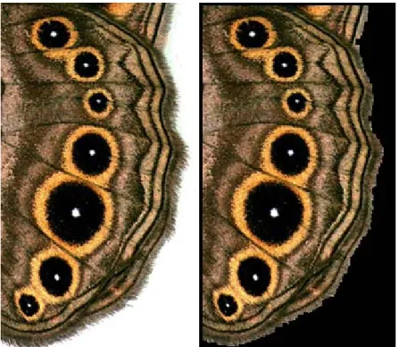
(21) Separation of each eyespot (wing) This section is only used for “Forewing” and “Hindwing” images and consists in separating the eyespots from each other in case there’s merging of neighbouring eyespots through the yellow area. This part of the program obtains the coordinates for each eyespot centre and draws dividing lines between each eyespot on the image with the skeletonized outlines of the binarized original image (fig. 8 – right image). . Figure 8: left – original image (bigeye mutant); centre – eyespot representation image; right – skeletonized outlines of the binarized original image with dividing lines. . Firstly the program has to check if the image contains a white background in order to eliminate it. This is required because the program searches for the white areas as the position reference for each eyespot. As the wing is round shaped, the most efficient and quick method to accomplish this is by inspecting each corner for white pixels. If there’s a white background, the image is binarized with a threshold of 128 (middle point in the gradient range of 256) and a great part of its smallest holes filled with the close operator, which is a morphological operator which is simply a dilation followed by an erosion, and the dilate operator. In spite of this processes and even if the ‘fill holes’ function is used, the wing still could have holes on the edges of the image, mainly because the ‘fill holes’ function searches the sides for the background colour so that it can identify the area outside the object that is going to have its holes filled. A work around for this possible problem is to make the program draw lines around the edges where the wing touches, by finding out where the white corners finish and the wing starts and drawing a line between them. After this, the ‘fill holes’ option is applied and all that is left is the white background and the black 10 .

(22) section of the wing. Then the image is inverted and framed with a white line around it, to account for small white pixels at the border of the wing which could be just at the edge of the image, followed by some dilation, also to account for the same possible problem. After all this steps, this image is added to the original one, overlapping the white background (fig. 9 – right image). . . Figure 9: left – original image; right – image without the white background. . The next step consists in finding each eyespot present. For this, the program will search for the white centre area pixels with the value given by the pixelLimit variable (equal to 255 to start with) for each colour. Once it’s found a pixel with that value, it is inserted in a blank image. After all the pixels have been analysed, the program investigates the blank image with the particle analyser function to see if there’s at least as much particles as there is eyespots, number that was provided by the user earlier in the second initial dialog. If this is false, the program then decreases the pixelLimit value by one and searches the pixels again, creating a new blank image for it. This process continues until the previous condition is true, and then it shows the result blank image with the possible locations for each eyespot and subsequently asks the user if it contains all of the eyespots present in the original image. If some of them aren’t in the correct position, it means that it’s a false eyespot, probably an error from the photography, and the program will have to analyse the image again to find the missing eyespot(s). After it has found all the eyespots, if there were false ones, the program asks the user to select with the mouse pointer the particles that correspond to the real eyespots (this is a user friendly input because the selection doesn’t have to be so accurate or sequential) and it will make a correspondence between those points selected and the nearest particle, followed by the sorting of the eyespots from top to bottom. If the user selects a different number of points than the number of eyespots, the program will alert the user to the situation, allowing him to correct this. 11 .

(23) The final step of the separation of the eyespots consists in drawing the dividing lines between them. First the program starts to make an image with the outlines of the binarized original image the same way the macroWork method do but without the skeletonize function, so that the outlines are continuous without diagonal breaks. To draw the line between two eyespots, the program needs to know what its slope is and where it is going to pass, which will be a point between the black area/ yellow area frontiers. To find out the latter, an imaginary line is drawn connecting the centres of the two eyespots to be analysed. Then, starting from each eyespot centre, the program will run along the line until it finds its frontier between the black and the yellow areas. The running process actually starts at 1/8th of the distance between the eyespots and if it found only one of the frontiers due to its absence or to poor quality of the image or even possibly the merging of the black areas, the program sets the passing point as the middle of the imaginary line. The other passing points, for “Hindwing” images, are set more or less near the frontiers, depending on the ratio between them, with some exceptions. This deviation from the centre of the zone between each black area/ yellow area frontier is necessary because by observing the images, we can perceive that the veins are closer to the frontier belonging to the biggest of the pair of eyespots. So by applying this ratio to the calculation of the passing point, the separation of the eyespots gets more accurate by mimicking the position of their natural dividers, the veins, and thus getting a more precise area value for each individual yellow area. For “Hindwing” images from mutated individuals with extra eyespots the value used for the ratio is 0.5, mainly because by having extra eyespots, their positions may cause problems with their normal arrangement and could cause the divisions to occur in odd places. In the case of a hind wing with seven (or even eight eyespots – although a mutant, this eyespot position don’t disrupt the normal layout of the rest) the ratios are treated differently for each case. For the first four eyespots, the ratio used to determine the position of the passing point is the calculated one and for the rest of the eyespots the ratio is 0.5 due to better division with this value than with the calculated one. The ratio of 0.5 is also used for all the other cases. After finding out the passing points for the lines, the program is going to calculate their slopes which is very straight forward since they’re perpendicular to the imaginary lines between the eyespots’ centres. Although logic dictates that for each pair of eyespots, these imaginary lines are suppose to be between the eyespots in question, we observe that most of the times, for hind wings, this doesn’t reflect the positions of the veins at all. So we found out that by using other eyespot to pair with the upper one of the pair, we get a more accurate line. Even though the veins are slightly curved, the lines almost exactly overlap their terminal portions where the eyespots are (see fig. 8). So when the program analyses “Hindwing” images and there’s seven or even eight eyespots present, the pairing are: the first with the fifth, the second with the fifth, the third with the sixth, the forth with the seventh, the sixth with the seventh, the seventh with the sixth again and, for the eighth 12 .

(24) eyespot, the seventh with the eighth. For the other cases, the slope is calculated using the eyespots that bracket them. In the end, with the values for the slope and the passing position, the program calculates the equations for the dividing lines and draws them over the skeletonized outlines of the binarized original image, which can be viewed if the user chooses to. . . 13 .

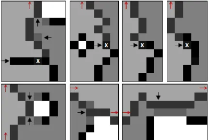
(25) Analysis of the eyespot Analysis of normal images This subsection is used when the “Single Eyespot”, “Forewing” or “Hindwing” option is selected during the first initial dialog. It’s the one that gives the user the outlines of each area and their data (area, roundness, diameter, area ratios and image representations) for normal eyespot or wing images. To obtain the frontiers of each eyespot, the program starts at its centre and moves along the pixel line to the right until it has found three frontiers (this method is performed for each eyespot in the case of a wing image). So first the program sets the eyespot centre coordinate. If it’s a wing image, the coordinate is set as the current eyespot to be analysed, found by the ‘separation of each eyespot (wing)’ section, and if it’s a “Single Eyespot” image, the coordinate is set as the centre of the image. Also in this latter case, the image is framed with a black line encased in an exterior colour line (more about colours later – also see fig. 11 for colour codes), to account for single eyespots that could be merged with another out‐of‐frame eyespot or for those that could be missing parts of its yellow area. Mainly because the “Single Eyespot” image could possibly not be centred properly on the image frame or to account for the possibility of some error with the outlines, the program now applies the findWhite method to this centre point, in order to find the closest white (or close to white) pixel. The findWhite method, which is found at the end of the program, returns a set of coordinates (x, y) from the original image, corresponding to the closest white (or close to white) pixel to the given set of coordinates. The value used to find this pixel is the pixelLimit variable discussed above. When the image type is “Single Eyespot”, the default value is set to 245 and not 255 to take into consideration the possibility of image quality error. This method works by comparing the pixels in a spiral motion (fig. 10) around the initial coordinate until one with all the three RGB values equal to the pixelLimit value or, in the case of a “Single Eyespot” image, until it reaches the limit of the frame. For wing images, this method doesn’t need to rely on this latter condition because it most certainly finds a pixel right at the initial coordinate. If either of the returned coordinates are zero, it means that it didn’t find the pixel, and so the program sharpens the image and tries again until it has found out a correct set of coordinates to start the search for the three frontiers properly. . 14 .

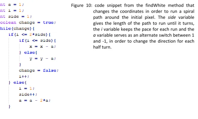
(26) Figure 10: code snippet from the findWhite method that changes the coordinates in order to run a spiral path around the initial pixel. The side variable gives the length of the path to run until it turns, the i variable keeps the pace for each run and the a variable serves as an alternate switch between 1 and ‐1, in order to change the direction for each half turn. . After the program has found the initial pixel, it paints the white area with its colour (more about colours later – also see fig. 11 for colour codes) and it starts the search for the frontiers of each area. To do this, the program runs along the x‐axis, starting from the previously obtained set of coordinates, until it finds a black pixel. When this occur, the program analyses the next pixel colour. If it’s white, then it most certainly is a possible frontier. If it’s another colour besides white or black, it’s most likely some black pixel or line that doesn’t make part of a frontier – the area outside the frontier is supposed to be a non‐ painted white area, so the program continues the search forward for another black pixel. After it has found a possible frontier, with a white area on the other side, the program runs along the frontier and registers each of its pixels onto a separate blank image corresponding to that area of the eyespot. This just cannot be done by simply find the next black pixel, going up or down, because there could be several black pixels or lines that go through the frontier and mislead the program and causing it to go the wrong way. The best way to avoid this is to simply give the program a sense of where it is along the line. The line that makes the frontier must be surrounded by a different area on each side. So to distinguish both sides, the program paints the next area with a different colour and simply follow some rules. The colours used are shown bellow. . Figure 11: colour scheme used to run through the frontiers. The first four colours are used for each or the areas: white area, black area, yellow area and exterior area. The other three colours are respectively: debris colour, line colour and initial pixel colour. . . 15 .