What has been driving the fluctuations in the portuguese economy? A business-cycle accounting approach

(1)

M

ASTER

M.S

C

.

IN

E

CONOMICS

M

ASTER

´

S

F

INAL

W

ORK

D

ISSERTATION

W

HAT

H

AS

B

EEN

D

RIVING THE

F

LUCTUATIONS IN THE

P

ORTUGUESE

E

CONOMY

?

A

B

USINESS

-

CYCLE

ACCOUNTING APPROACH

F

REDERICO

F

IGUEIROA

T

EIXEIRA DE

A

BREU

(2)

M

ASTER

M.S

C

.

IN

E

CONOMICS

M

ASTER

´

S

F

INAL

W

ORK

D

ISSERTATION

W

HAT

H

AS

B

EEN

D

RIVING THE

F

LUCTUATIONS IN THE

P

ORTUGUESE

E

CONOMY

?

A

B

USINESS

-

CYCLE

ACCOUNTING APPROACH

F

REDERICO

F

IGUEIROA

T

EIXEIRA DE

A

BREU

S

UPERVISION

:

L

UÍS

F

ILIPE

P

EREIRA DA

C

OSTA

P

EDRO

M

IGUEL

S

OARES

B

RINCA

(3)

GLOSSARY BCA – Business-Cycle Accounting.

CKM – Chari, Kehoe, and McGrattan, i.e. Chari et al. (2007). GDP – Gross Domestic Product.

RBC – Real Business Cycles. TFP – Total Factor Productivity.

(4)

FREDERICO ABREU FLUCTUATIONS IN THE PORTUGUESE ECONOMY

ii

ABSTRACT,KEYWORDS AND JELCODES

Abstract

The Portuguese economy has been submitted to a thorough evaluation by the scientific community, in a search to explain the Portuguese “lost decade” and, more recently, the sovereign-debt crisis following the Great Recession.

In this dissertation I measure and evaluate the fluctuations in the Portuguese economy using the Business-Cycle Accounting (BCA) method. I especially focus on three sub-periods that span from 1992 to the present day. I also provide some context on the shape of the Portuguese economy, mainly by checking what were the biggest obstacles to growth according to the literature.

Applying the BCA procedure to the Portuguese economy led to the conclusion that the investment wedge had the largest role in explaining the fluctuations of the economy as a whole for both the 1992-2001 and 2007-2014 periods and that the efficiency wedge played a major role in the 2001-2007 slump. According to Portugal and Blanchard (2017) there is a cycle throughout 1992-2013. The period studied on this dissertation will focus on this cycle and its boom, slump and recession sub-periods.

The conclusions obtained are somewhat different from those in the previous BCA literature on the Portuguese economy. Namely, the efficiency wedge is the main explainer in both Iskrev (2013) and Cavalcanti (2007), although providing a similar result to the period in study they disregard the importance of the investment wedge.

Keywords

Investment wedge, Efficiency Wedge, Labor Wedge, Government Wedge, Business Cycle Accounting, Portuguese Economy, Great Recession

JEL Codes

(5)

CONTENTS

Glossary ... i

Abstract, Keywords and JEL Codes ... ii

Abstract ... ii Keywords ... ii JEL Codes ... ii Contents ... iii Table of Figures ... v Table of Tables ... vi Acknowledgements ... vii 1. Introduction ... 1

2. The Business-Cycle Accounting Technique ... 3

2.1. The model ... 3

2.2. Applying the method ... 5

3. Mapping the wedges for Portugal ... 8

3.1. Data ... 8

3.2. Method... 8

3.3. Benchmark wedges and their components throughout the three periods ... 10

3.3.1. The Boom (1992:I – 2001:I) ... 12

3.3.2. The Slump (2001:I – 2007:I) ... 15

3.3.3. The two crises (2007:I – 2014:IV) ... 18

4. Relevant Wedges and Plausible Narratives ... 22

4.1. The Efficiency Wedge ... 22

4.1.1. The combined Efficiency and Labor wedge economy ... 23

(6)

iv

4.2.1. The combined efficiency, labor and investment wedge economy

... 24

5. The Literature on the Portuguese economy ... 26

5.1. The Boom (1992 – 2001) ... 26

5.2. The Slump (2001 – 2007) ... 27

5.3. The Two Crises (2007 – 2014) ... 28

6. Conclusion ... 30

References ... 32

(7)

TABLE OF FIGURES

FIGURE 1-DE-TRENDED PER CAPITA MACROECONOMIC VARIABLES IN THE DATA (LOG-LINEAR FILTER) 10 FIGURE 2-OUTPUT AND ITS COMPONENTS OF EACH SINGLE-WEDGE ECONOMY FOR THE BOOM (1992:I

–2001:I) ... 12 FIGURE 3-OUTPUT DATA AND THE OUTPUT COMPONENTS OF A ONE WEDGE OFF MODEL FOR THE

BOOM (1992:I–2001:I) ... 14 FIGURE 4-OUTPUT AND ITS COMBINED-WEDGE MODELS FOR THE BOOM (1992:I–2001:I) ... 15 FIGURE 5- DATA OUTPUT AND OUTPUT COMPONENTS OF EACH SINGLE-WEDGE ECONOMY FOR THE

SLUMP (2001:I–2007:I) ... 16 FIGURE 6-OUTPUT FROM THE DATA AND THE ONE WEDGE OFF MODELS OUTPUT COMPONENTS FOR THE

SLUMP (2001:I–2007:I) ... 17 FIGURE 7-OUTPUT AND THE COMBINED WEDGE MODEL’S OUTPUT COMPONENTS FOR THE SLUMP

(2001:I–2007:I) ... 18 FIGURE 8-OUTPUT COMPONENTS OF EACH SINGLE-WEDGE ECONOMY TOGETHER WITH THE ACTUAL

OUTPUT FROM DATA (DETRENDED) THROUGHOUT TWO CRISES (2007:I–2014:IV) ... 19 FIGURE 9-THE ONE WEDGE OFF MODEL’S OUTPUT COMPONENTS AND DATA OUTPUT THROUGHOUT THE

TWO CRISES (2007:I–2014:IV) ... 20 FIGURE 10-COMBINED TWO WEDGE MODELS’ OUTPUT COMPONENT AND ACTUAL OUTPUT

THROUGHOUT THE TWO CRISES (2007:1–2014:4) ... 21 FIGURE 1A-THE BOOM DATA OUTPUT AND THE SINGLE-WEDGE ECONOMIES OUTPUT COMPONENTS ... 35 FIGURE 2A-THE SLUMP DATA OUTPUT AND THE SINGLE-WEDGE ECONOMIES OUTPUT COMPONENTS . 35

FIGURE 3A-THE TWO CRISES DATA OUTPUT AND THE SINGLE-WEDGE ECONOMIES OUTPUT

(8)

vi

TABLE OF TABLES

TABLE I- STATISTICS OF THE SINGLE-WEDGE ECONOMY OUTPUT, LABOR, INVESTMENT, AND

CONSUMPTION COMPONENTS REGARDING THE BOOM (1992:I–2001:I) ... 13 TABLE II- STATISTICS OF THE ONE WEDGE OFF MODELS AND THEIR COMPONENTS FOR THE BOOM

(1992:1–2001:1) ... 14 TABLE III-STATISTICS OF THE SINGLE-WEDGE ECONOMY OUTPUT, LABOR, INVESTMENT, AND

CONSUMPTION COMPONENTS REGARDING THE BOOM (1992:I–2001:I) ... 16 TABLE IV- STATISTICS OF THE ONE WEDGE OFF MODELS AND THEIR COMPONENTS FOR THE SLUMP

(2001:1–2007:1) ... 17 TABLE V-STATISTICS OF THE SINGLE-WEDGE ECONOMY OUTPUT, LABOR, INVESTMENT, AND

CONSUMPTION COMPONENTS REGARDING THE TWO CRISES (2007:I–2014:IV) ... 19 TABLE VI- STATISTICS OF THE ONE WEDGE OFF MODELS AND THEIR COMPONENTS FOR THE SLUMP

(2001:1–2007:1) ... 20 TABLE IA-STATISTICS OF THE SINGLE-WEDGE ONLY MODELS’ OUTPUT COMPONENTS FOR THE THREE

(9)

ACKNOWLEDGEMENTS

I would like to thank my family for the support and pressure given to help me keep up with the discipline and hard work required to finish a dissertation. I would also like to thank the supervisor, Luís F. Costa, who has been an exemplary mentor with a keen critical spirit, and Pedro Brinca, for providing me with the means and knowledge to apply the BCA method.

(10)

1

WHAT HAS BEEN DRIVING THE FLUCTUATIONS IN THE PORTUGUESE ECONOMY? A BUSINESS CYCLE ACCOUNTING APROACH

By Frederico T. Abreu

IN THIS DISSERTATION I measure and evaluate the fluctuations in the Portuguese economy using the Business-Cycle Accounting method. I especially focus on three periods from 1992 to the present day. The result of this application led to the conclusion that the investment wedge had the largest role in explaining the fluctuations of the economy as a whole for both the 1992-2001 (Boom) and 2007-2014 (Two Crisis) periods and that the efficiency wedge played a major role in the 2001-2007 (Slump).

1. INTRODUCTION

Since the Great Recession, there has been a large volatility in the Portuguese economy: be it on GDP and its components or in employment and productivity. These fluctuations inspired curiosity in the scientific community and many tried to study their causes. This dissertation aims to shed a light on the possible explainers of these fluctuations throughout the period 1992-2015 using a Real Business Cycle (RBC) model.

In order to answer the research question, I use the Business-Cycle Accounting (BCA) method, developed by Chari et al. (2007) and recently surveyed in Brinca et al. (2016). The method involves using a benchmark RBC model to map frictions in the first-order conditions, which are also known as wedges. Four wedges are considered, each one related to a variable in the model: investment, efficiency, government expenditure, and labor.

The BCA method has been widely used to answer questions of the same nature as that of this dissertation. Chari et al. (2007) applied the BCA method to the US in the Great Depression, Cunha (2006)1_{applied it for Japan during the “lost decade”. Cavalcanti}

(2007), Iskrev (2013), and Caraiani (2016) applied it to Portugal. Finally, Brinca et al. (2016) applied the method to several OCDE countries.

The main conclusion for the 2007:I – 2015:IV and the 1992:I – 2001:I periods is that the one wedge-model that best reproduces output time series is the one with an investment wedge only. This result differs from the previous literature such as Iskrev (2013) that applies the BCA method to Portugal in a coinciding period. In the period 2001:I – 2007:I the efficiency wedge only economy was the best simulator for actual

(11)

output and this is consistent with previous literature such as Iskrev (2013), Cavalcanti (2007) and Carianari (2016).

I also found that the literature on the Portuguese economy, for both the pre- and post-crisis periods, was more focused on productivity and labor market issues than in investment related ones. Taking this into account, I will analyze the previous literature in detail and I will highlight the differences in the results obtained.

In chapter 2, I begin by defining the BCA method and exposing the RBC benchmark model. In chapter 3, I will apply the BCA method to study the fluctuations in the Portuguese economy throughout its three main periods and to uncover the set of wedges that best explains the fluctuations in the Portuguese economy. The three periods are named and selected in accordance to Blanchard & Portugal’s (2017) perspective of the business cycles in Portugal. In chapter 4, I explore the links that may exist between the wedges and possible economic explanations, i.e. specific theoretical models. Finally, in chapter 5, I provide some context by exploring the existing literature on the Portuguese economy. Finally, Chapter 6 concludes and summarizes on the previous chapters.

(12)

3

2.THE BUSINESS-CYCLE ACCOUNTING TECHNIQUE

In this chapter, I present the BCA method to be used. The technique consists in using a benchmark prototype economy to find the wedges between the model’s artificial data generate by its first-order conditions and actual data. There have been different ways of applying this technique, in this case, I follow both Brinca et al. (2016) and Chari et al. (2007).

2.1. The model

The benchmark model is a stochastic growth model with an endogenous labor-supply decision, i.e. an RBC model. Several specific models are presented together with the equivalence results for each wedge in the prototype model, as in Chari et al. (2007).

In each period t, the economy is affected by one of finitely many events, denoted 𝑠𝑡 = (𝑠₀, … , 𝑠_𝑡) with probability function 𝜋_𝑡(𝑠𝑡), which means the probability of history 𝑠𝑡 is 𝜋𝑡(𝑠𝑡) . The initial event 𝑠0 is given.

The model has four exogenous stochastic variables, which are all functions of 𝑠𝑡

and represent the four wedges through distortions in the economy’s first-order conditions: the efficiency wedge 𝐴_𝑡(𝑠𝑡), the labor wedge 1 − 𝜏_𝑙𝑡(𝑠𝑡), the investment wedge

1/ (1xt( ))st , and the government-consumption wedge, which is just the residual for the

sum of government final expenditure and net exports, 𝑔_𝑡(𝑠𝑡). The economy is assumed to have homogeneous consumers, where each one chooses per capita consumption (𝑐𝑡)

and per capita labor (𝑙_𝑡) to maximize the intertemporal discounted utility function: (1) 0 t ( ) ( ( ), (s )) t t t t t t t t s



s U c s l N   

 

,

subject to a budget constraint:

(2) 1

( )t (1 (s )) x ( )t t (1 ( ))t ( ) ( )t t ( ) (t t ) ( )t

t xt t lt t t t t t

c s   s   s w s l s r s k s T s , and to the capital-accumulation law of movement:

(3) 1 1 (1 ) ( )t (1 ) ( t ) ( )t n kt s k st x st         ,

where U(•) is the utility flow, per capita capital stock is denoted by 1

( t )

t

k s , x st( )t

represents per capita investment, w st( )t is the wage rate, ( )

t t

r s stands for the rental rate on capital, t is the discount factor,  represents the depreciation rate of capital, N _t

(13)

is the population with growth rate  , and _n T st( )t stands for per capita lump-sum

transfers.

The production function has the form 1

( ) ( (t t ), (1 )t ( ))t

t t t

A s F k s  l s , where  is the

rate of labor-augmenting technical progress, assumed to be constant. The firm’s profit

function is given by 1 1

( ) ( (t t ), (1 )t ( ))t ( ) (t t ) ( ) ( )t t

t t t t t t

A s F k s  l s r s k s w s l s . The equilibrium for this benchmark prototype economy is obtained with the resource constraint:

(4) ( )t ( )t ( )t ( )t

t t t t

c s x s g s y s ,

where y st( )t denotes per capita aggregate output and gt(s

t_{) stands for the sum of public}

final expenditure and net exports, both measured in per capita terms, together with

(5) 1 ( )t A ( ) ( (t t ), (1 )t ( ))t t t t t y s  s F k s  l s , (6) ( ) [1 ( )] ( )(1 ) ( ) t t t t lt lt t lt t ct U s s A s F U s       , (7)





1 1 1 1 1 1 1 1 1 1 ( )[1 ( )] ( | ) ( ) ( ) ( ) (1 ) 1 ( ) t t t ct xt t t t t t t t ct t kt xt s U s s s s U s A s F s s                      _  _



,

where U ,_lt U ,_ct F , and _lt F represent the first partial derivatives of the utility and _kt

production functions with respect to their arguments, and _t(st1|st) = 1

( t ) / ( )t

t s t s

  

. Furthermore, I assume that g st( )t fluctuates around a deterministic trend g0(1 )

t

  . By looking at equations (4) to (7) we can observe that each wedge represents a distortion in the first-order conditions of the model. Thus, taking the labor wedge

1_lt( )st as an example, it represents failures in the labor market that correspond to the distortions on the first-order contemporaneous condition (6), which resemble taxes on labor income. In this sense, the labor and investment wedges [1/ (1xt( ))st ] are similar.

The efficiency wedge is reflected in the total factor productivity (TFP), which, when normalized to 1, has a distortion A ( )t st . Finally, the residual-demand wedge ( )

t t

g s

represents both government consumption and net exports’ impact on total demand. Using the same method as in Brinca et al. (2016), here also the capital-accumulation law (3) is replaced, to include investment adjustment costs, by

(14)

FREDERICO ABREU FLUCTUATIONS IN THE PORTUGUESE ECONOMY 5 (8) 1 1 1 ( ) (1 ) ( ) (1 ) ( ) ( ) ( ) t t t t t n t t t t t x s k s k s x s k s             _{ } _   ,

where  is the capital stock adjustment cost per unit, which is defined as

(9) 2 , 2 x a x b k k  _{ } _  _    

with b   representing the steady -state value for the investment-capital ratio.   _n 2.2. Applying the method

Let us consider the theoretical model in section 2.1. I assume, in line with Chari et al. (2007), henceforth CKM, and Brinca et al. (2016), a Cobb-Douglas production function with constant returns to scale: F k l( , )k l 1, with 0 <  < 1. Furthermore, I

assume an additively-separable logarithmic utility function:

U c l

( , ) log



c





log(1- )

l

. For the parameter values, I used those in Brinca et al. (2016), which are in accordance with traditional BCA and macroeconomic literature: (i) the capital share in aggregate income, for simplicity, is calibrated to  = 1/3, so that the share of capital in aggregate income is 0.33;2 (ii) the time-allocation parameter is  = 2.5 so that labor has a steady state value of 2222 annual hours worked per capita, far from the average of 1990 obtained from the data on Portugal for 1992-2014; (iii) the depreciation rate  = 0.05, i.e. a 5 per cent depreciation in annual terms, which fits the Portuguese data that shows a 5.5% real depreciation rate3 ; and (iv) the discount factor  = 1/1.025, i.e. a 2.5 per cent rate of time preference per quarter. Growth rates  and  n are both computed such that

the previous two parameters fit the given values. The adjustment-cost parameter a is such that the elasticity of the price of capital with respect to the investment-capital ratio is  = 2.5. Notice that the price of capital is

q



1/ (1





')

, which, at steady state, means that

ab





. Thus, given the values for b and , a is set accordingly4_.

2_{This assumption was made for simplicity, based on previous literature (Brinca et al. 2016), the real}

share of wages in aggregate income is around 0.53, suggesting a capital share of 0.47, calculated using data from European Comission (2018)

3_{This value was obtained using data from European Commission (2018)}

4_{Given the difference between the reality in the data and the parameters chosen here, I decided to}

(15)

The state

s

t is assumed to follow a first-order Markov process. I also assume a ne-to-one mapping between the states and the wedges, which means that for any event st, we have A s_t( )t s_At, _lt( )st s_lt, _xt( )st s_xt, and ( )t

t gt

g s s .

To estimate the stochastic process, I use the following first-order autoregressive (AR(1)) process, for the event st (sAt,s slt, xt,sgt):

(10) s_t_₁ P₀Ps_t _t_₁,

with _t_₁ being i.i.d and normally distributed, with mean 0 and covariance matrix V. Let (y l_td, _td,x_td,g_td,k₀d) denote respectively the data at time t for output, hours worked, investment, the sum of government consumption to net exports, and capital stock at time 0. Additionally, let ( ,y s k , ( ,_t _t) x s k , ( , )_t _t) l s k denote the decision rules of the model, _t _t

obtained from equations (5)-(7). The government wedge can be obtained directly from equation (4). Both the labor and efficiency wedges are directly obtained from equations (5) and (6). Finally, the investment wedge in equation (7) has to be estimated through a process that will be described in section 3.2. One should notice that that all these wedges put together will replicate the data fully, since they are obtained by using the system of equations (4)-(7). The resulting wedge series d

t s will solve (11) d ( d, ) t t t y y s k , d ( d, ) t t t x x s k , and d ( d, ) t t t l l s k ,

together with the actual capital-accumulation law of motion in equation (8), ₀d o

k k , and

d t t

g g . Finally, I use this equation (8) together with the system of equations (5)-(7) to uncover the values for the state vector and obtain the wedges.

Once the wedges are obtained, we can evaluate their marginal effects through simulation experiments. I use the single-wedge economies in which the equations (5)-(7) are used to uncover the output, labor, and investment allowing only that wedge to vary and setting the others constant. To exemplify, the effects of the efficiency wedge could be measured by calculating the efficiency-wedge alone economy decision rules, denoted

directly, and ψ is chosen to obtain the actual average for annual hours worked per capita of 1990. The result lead to similar conclusions to the actual parameters exercise as shown in the appendix.

(16)

7

by y_At ( ,s k_t _t), l_At ( ,s k_t _t), and x_At ( ,s k_t _t), by allowing the efficiency wedge to vary freely, i.e. A st( )t sAt, while setting the other wedges to ( )

t lt s l

  , _xt( )st _x, and g st( )t g, which are obtained via the unconditional mean of the AR(1) process

1 0

(IP) P, with I being the identity matrix and matrices P and P0 are given by equation

(10). To the results of these key decision rules, I will call respectively the efficiency-wedge output, labor, and investment components. The same nomenclature will be applied to all single-wedge economies. In addition, I will use one-wedge-off models, which work in the opposite way to single-wedge models: I will allow every wedge except one to vary and keep the value of the off wedge at its unconditional mean. Finally, I will build a pair of combined-wedge models: (i) one that allows both the labor and the efficiency wedge to vary and sets the other two at their mean and (ii) one that allows both the investment and the government wedge to vary, but the efficiency and labor wedges are set at their mean.

(17)

3.MAPPING THE WEDGES FOR PORTUGAL

3.1. Data

In order to collect the relevant macroeconomic data5, I start using the Banco de Portugal (2016) quarterly database, henceforth mentioned as BdP database. The list of variables used amongst the available ones were: nominal GDP, investment, private consumption, government consumption, imports and exports of goods and services, and the GDP deflator (2008: IV = 100). However, hours worked per employee and total population in working age (ages 15-65), were obtained from OECD (2015)6 and Pordata (2017) respectively.

3.2. Method

For measuring the wedges, I used the MATLAB code provided in Brinca et al. (2016), which was applied to several OECD countries, Portugal not included, with small alterations to fit it into my data. For the main macroeconomic variables in the BdP database, I used the GDP deflator to obtain real output, private consumption, investment, and government consumption (including the trade balance). The reason for using a single deflator instead of variable-specific deflators is that according to the benchmark model there is only one good.

Given the fact that data for working-age population was only available from Pordata at annual frequency, I used a cubic spline to interpolate quarterly observations. To do so, I assumed that between two years, the population did not cross neither the upper nor the lower bounds given by annual observations. In other words, I assumed the variable changed smoothly and slowly between two periods, which seems to be a plausible assumption for this historical period in the Portuguese economy.

The macroeconomic real data from the BdP database and hours worked per employee from OECD is firstly divided by working-age population (group aged 15-65)

5_{Here follows the link to the database with the compound raw data used:} https://www.dropbox.com/sh/hpbzsg89lwlbjyc/AABt0KgAD6f3Nti8ucocUAfia?dl=0

(18)

9

to obtain per capita values.Then, I de-trended the variables using a log linear filter. De-trended per capita variables were then used as an input for the MATLAB code.

Unlike the other wedges, that can be directly obtained from the system of equations (5)-(7), the investment wedge deals with expectations of future consumption, which are assumed to follow a stochastic process. The code estimates the investment wedge using the maximum-likelihood method, given the restrictions imposed by the other wedges, to solve the system of equations (5)-(7). Once computed or estimated, the wedges are then singled out by allowing only a set of them to move while keeping the others constant, to study their ability to replicate actual output, consumption, hours worked, and investment. Usually in BCA, the correlation coefficient is used to identify the most important wedges. However, I will use the  statistic, defined in Brinca et al. (2016). This statistic, which ranges between 0 and 1, has the benefit of adding to one across all wedges, which reveals the relative importance of each wedge in tracking the data on output, consumption, hours or investment, using single-wedge models. This statistic also tracks how close the two series (simulated and actual) move, through the local distances between both. The  statistic can be considered more accurate, since it measures point specific accuracy instead of the correlation’s overall co-movement accuracy. The definition of the  statistic for output (an example) is given by

(12) 2 2 1/ ( ) , (1/ ( ) ) t it Y t i t jt j t y y y y    





where yt stands for actual output and yit (yjt) is the output component generated by the

one wedge on model for wedge i j, 



z l x g, , ,



, For simplicity on graphs and tables, from here on the wedges shall have the following notation: instead of A I will use z for the efficiency wedge; l stands for l; x represents for x; and g still represents the

government consumption wedge. this same notation is used in the one wedge off model, in which case each letter will let us know which wedge is off (not allowed to vary) rather than on. This can also be done to combined wedges using the following for two wedge models: i j, 



zl xg,



. In the case of two wedge models the following notation is used: zl

(19)

for the combined labor and efficiency wedges on model, and xl for the combined investment and government wedges on model.

3.3. Benchmark wedges and their components throughout the three periods

Before moving on this section, a guideline for notation in the tables and figures: the letters z, l, x, and g are respectively the efficiency, labor, investment and government wedges. All figures will have output components of models that allow a subset of these wedges to vary while the others are kept constant. To exemplify the output component of the efficiency wedge on model will be noted as yz. In the case of the one wedge off model’s the same notation will be used. The combined efficiency and labor wedge model’s output component is yzl. When it comes to tables it is easier since they will show for both the one wedge on and the one wedge off model the  statistics of each model’s component.

To give out some context let us review some relevant Portuguese data.

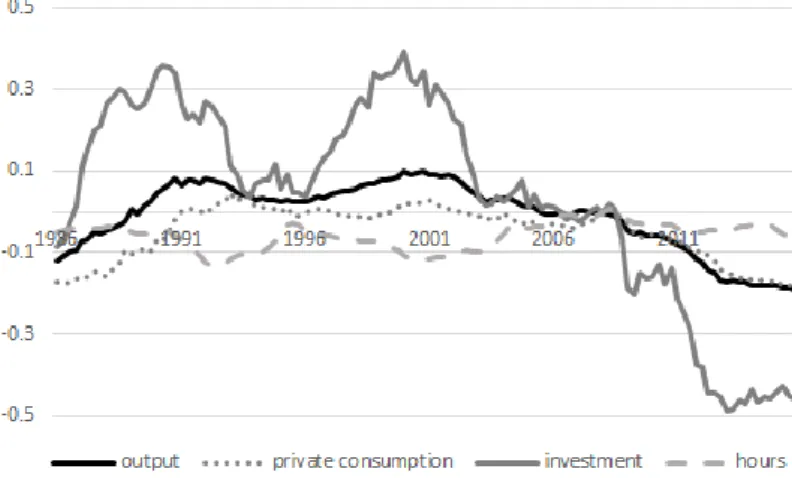
FIGURE 1 - DE-TRENDED PER CAPITA MACROECONOMIC VARIABLES IN THE DATA (LOG-LINEAR FILTER)

The map of each quarter in the figures is as follows: first quarter of 1986 is 1986, the second 1986.25, the third quarter 1986.5, and the last is 1986.75. This format for the periods is used on the remaining figures.

Figure 1 depicts the de-trended per capita variables (output, consumption and investment), all normalized to the first quarter in the year of the Great recession, 2008. The hours worked per capita, are only normalized to the first quarter of 2008.

(20)

11

as ss) which is at 1, in this exercise I subtracted 1 to all values to purely get the percentage deviation from the ss. These variables are the result of applying the GDP deflator to output, consumption, investment and hours, then divide it by the population in working age (ages 15-65), and finally applying a log-linear filter to them. The log linear filter consists of three steps: calculate the logs of the variables, make a linear regression with time as the dependent variable, which will provide the trend line, and finally subtract the trend from each quarter’s value. By applying the log-linear filter the variables will show a cycle around their trend, which allows me to analyze their fluctuations around their trend. The ss is at 0, and each movement of 0.01 in one direction is a deviation of 1 per cent from the steady state. In this figure 1 investment shows two peaks well above trend on the third quarter of 1990 and on the first quarter of 2000. In the case of GDP, it can be observed that 2000-2002 represented a turning point for the Portuguese economy. Following the proposition for the business cycle provided in Blanchard & Portugal (2017), the business cycles seem to have had a boom in the period 1995-2001, then a slump between 2002-2007, which is followed by a constant downward path until the end of the series.

In the case of consumption, we can observe that the series is almost identic to that of GDP, which shows pro-cyclicality, with a lag. The contemporary correlation between GDP and consumption (0.87) is slightly smaller than the lagged correlation between consumption and previous period GDP (0.9), and as I increase the lag by one period the correlation increases. Consumptions shows a smaller variation than GDP, with a standard deviation of the former on 0.06 compared with the latter’s 0.08.

Investment, just like consumption, shows a pro-cyclical behavior, but exhibiting a larger variability, with investment showing a standard deviation of 0.24, the highest of these variables, being clearly the most penalized variable by the 2008 crisis, in terms of distance to the steady state.

Finally, hours worked show a slight counter-cyclical behavior, with a correlation of roughly -0.5 with GDP, by the graph it can be derived that there is a counter-movement performed by the hours worked when compared to output.

(21)

What follows are three sections related to the three periods of the business cycle of the Portuguese economy as seen by Blanchard & Portugal (2017)7: the first period named the Boom includes 1992:I-2001:I; the second period called the slump, goes from 2001:I – 2007:I, and the third period, called the two crises, from 2007:I – 2014:IV. In those sections, I will evaluate the three period’s wedges and the various models’ simulation for the variables mentioned in Figure 1 and compare throughout the different models which are the best at tracking each variable.

3.3.1. The Boom (1992:I – 2001:I)

As it can be seen in Figure 2, both output components produced by the efficiency-only and investment-efficiency-only wedges efficiency-only models behave pro-cyclically. The labor-wedge output component, in the first half of this first period, has a counter-cyclical behavior, but then around 1997 starts to behave pro-cyclically. Finally, the government wedge behaves purely in a counter-cyclical manner.

FIGURE 2- OUTPUT AND ITS COMPONENTS OF EACH SINGLE-WEDGE ECONOMY FOR THE BOOM (1992:I–2001:I)

Below I will show in Table I the numerical support to my graphical analysis of Figure 2. Table I below shows the values for the  statistics regarding this period’s data:

7_{It should be noted that I adjusted the Blanchard & Portugal’s (2017) business cycle periods so that}

(22)

13 TABLE I

 STATISTICS OF THE SINGLE-WEDGE ECONOMY OUTPUT, LABOR, INVESTMENT, AND CONSUMPTION COMPONENTS REGARDING THE BOOM (1992:I–2001:I)

statistics z l x G

Output 0.15 0.03 0.75 0.07

Hours 0.50 0.09 0.15 0.26

Investment 0.21 0.05 0.67 0.07

Consumption 0.04 0.59 0.23 0.14

The results obtained for the  statistics in Table I show a very important investment wedge, which is very surprising considering existing literature. Chari et al. (2007) themselves confess they only expect this wedge to have a tertiary role. Cavalcanti (2007), who analyzed a period right before this one (1979–2000) and compared the Portuguese economy to that of the US, concluded that both the labor and the efficiency components were the most significant, up to 2000, with the labor wedge only model emerging as a significant explainer of output variations. However, Cavalcanti (2007) used the correlation coefficient instead of the  statistic, which may explain the different results. As mentioned above, the labor component becomes pro cyclical, co-moving with output in the late 1990s, which is in line with Cavalcanti’s observations. Still, the fact that here the investment wedge has an overwhelming performance when tracking output as compared to the other wedges, might change our perspective on which are the main frictions that explain the evolution of output throughout this period8.

8_{It should be noted as a disclaimer that I consider consumer durables as investment rather than private}

consumption, which can help explain the investment wedge’s new importance in tracking output when comparing to previous literature.

(23)

FIGURE 3 - OUTPUT DATA AND THE OUTPUT COMPONENTS OF A ONE WEDGE OFF MODEL FOR THE BOOM (1992:I–2001:I)

Figure 3 shows that the simulation of the model that allows every wedge to vary except the government wedge is the best performer in tracking output. We can also observe that the model without the efficiency wedge is the worst tracker of output. This could be justified with the efficiency wedge model performance by the end of the period, where it becomes the best simulator of output. The relative measure of performance of each one wedge-off model in tracking output is shown in the table below.

TABLE II

 STATISTICS OF THE ONE WEDGE OFF MODELS AND THEIR COMPONENTS FOR THE BOOM (1992:1–2001:1) statistics z l x G Output 0.04 0.06 0.08 0.82 Hours 0.90 0.01 0.01 0.08 Investment 0.19 0.14 0.04 0.63 Consumption 0.04 0.09 0.81 0.06

As Table II tells us, there is no doubt that the government wedge off economy is the best tracker of output and investment, with all the others exhibiting a poor performance on tracking actual output. The efficiency wedge off economy is by far the best simulator of hours worked and the investment wedge off economy is the best on tracking consumption in the data.

(24)

15

FIGURE 4- OUTPUT AND ITS COMBINED-WEDGE MODELS FOR THE BOOM (1992:I– 2001:I)

In Figure 4, actual output and its simulation produced by combined-wedge models are depicted. The figure shows output in black, the combined labor and efficiency wedges on model’s output component in bright grey (yzl) and the combined government and investment wedges on model’s output component in dark grey (yxg). These output components are the simulations produced by a model where only a specific subset of wedges are allowed to vary, while keeping the remaining constant. Here, the subset is composed by two wedges, hence there are only two models. In this period, the model combining government and investment wedges is the best tracker of actual output. In fact, the  statistic for this model is 0.75, with the remaining 0.25 belonging to the output simulation produced by the model combining the efficiency and labor wedges.

3.3.2. The Slump (2001:I – 2007:I)

When I analyze Figure 5 throughout the Slump period, I observe that the efficiency-wedge output component is the best tracker of output. The investment efficiency-wedge only economy also produces a procyclical behavior, but its output component is far from the actual data. The labor wedge only economy generates an output that is countercyclical with the data and the government wedge economy produces a constant output level that is not consistent with the falling output observed in the data. To confirm these results, I show the  statistics in Table III for the Slump period.

(25)

FIGURE 5 - DATA OUTPUT AND OUTPUT COMPONENTS OF EACH SINGLE-WEDGE ECONOMY FOR THE SLUMP (2001:I–2007:I)

My observations to Figure 5 may now be put to test by Table III measuring the proximity between the simulated wedge economies and real data.

TABLE III

STATISTICS OF THE SINGLE-WEDGE ECONOMY OUTPUT, LABOR, INVESTMENT, AND CONSUMPTION COMPONENTS REGARDING THE BOOM (1992:I–2001:I)

statistics z l X g

Output 0.89 0.05 0.04 0.02

Hours 0.26 0.33 0.36 0.05

Investment 0.48 0.18 0.19 0.15

Consumption 0.79 0.10 0.04 0.07

These results lead to the conclusion that this crisis was mainly caused by a productivity shock, the same conclusion that Iskrev (2013) takes on his evaluation of the period (1998 – 2012), which includes the period under analysis and goes a bit beyond. However, Iskrev suggests a growing importance of the labor and investment wedges in the end of the period. Up to 2007, the efficiency wedge only economy has a remarkable precision on replicating actual output when compared to the others. To generate a behavior similar to that of hours worked, the investment wedge only economy, closely followed by the labor wedge economy are the best trackers. They also have an equal

(26)

17

replicates investment more accurately. In this period, the efficiency wedge only economy has a very significant importance for explaining both output and consumption behavior, a moderate importance when explaining investment, and a poor performance explaining hours worked.

FIGURE 6 - OUTPUT FROM THE DATA AND THE ONE WEDGE OFF MODELS OUTPUT COMPONENTS FOR THE SLUMP (2001:I–2007:I)

Figure 6 shows the investment wedge off model as the best tracker of output in this set of models, and the efficiency wedge model as the worst. This is consistent with the fact that the efficiency wedge only model has a strong performance in tracking output. This finding can be confirmed by the Table IV below.

TABLE IV

 STATISTICS OF THE ONE WEDGE OFF MODELS AND THEIR COMPONENTS FOR THE SLUMP (2001:1–2007:1) statistics z L x G Output 0.03 0.17 0.48 0.32 Hours 0.88 0.02 0.06 0.04 Investment 0.05 0.23 0.09 0.63 Consumption 0.02 0.07 0.81 0.10

As Table IV shows, the best trackers of output and consumption are the investment wedge off model, followed by the government wedge off model. When it comes to consumption, it remains almost the same as in the Boom. The best tracker of hours worked also remains the same as in the Slump, with an overwhelming performance by the

(27)

efficiency wedge off model when compared to others. Investment is best tracked by the government wedge off model.

FIGURE 7-OUTPUT AND THE COMBINED WEDGE MODEL’S OUTPUT COMPONENTS FOR THE SLUMP (2001:I–2007:I)

In Figure 7 the combined wedge model’s output components are shown together with the output from the data. There is no doubt that the combined efficiency and labor wedge model have a great performance, with a bit of a lag, at tracking output with a  statistics at an overwhelming 0.97. The combined investment and government wedge model’s output component shows an indifference to the fall experienced by the actual output in the data.

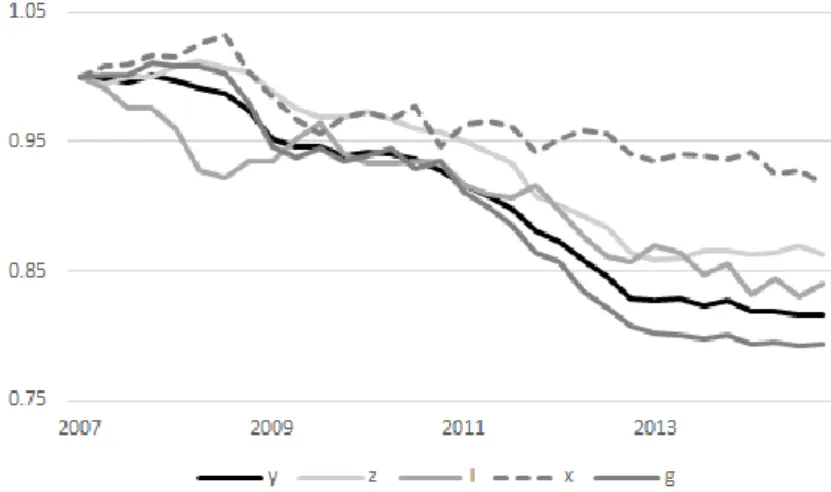
3.3.3. The two crises (2007:I – 2014:IV)

Now, I analyze the two crises period in Figure 8. We can observe that output falls, giving continuity to what we already see happening in the end of the slump. Even though the fall in output is continuous from the start of the Slump until the end of the two crises, I separate the two periods in this analysis. Figure 8 shows that the investment wedge only economy is the best tracker of output in data over this period, in contrast with the precise simulation generated by the efficiency wedge economy in the Slump. In the beginning of the period, the efficiency wedge only economy still shows promise in its simulation, but around the fourth quarter of 2008 the investment wedge only economy becomes undoubtedly the most reliable tracker of output until the end of the period.

(28)

19

FIGURE 8 - OUTPUT COMPONENTS OF EACH SINGLE-WEDGE ECONOMY TOGETHER WITH THE ACTUAL OUTPUT FROM DATA (DETRENDED) THROUGHOUT TWO CRISES (2007:I– 2014:IV)

After analyzing the period’s single wedge models graphically let us see what the analytical results are below on Table V:

TABLE V

STATISTICS OF THE SINGLE-WEDGE ECONOMY OUTPUT, LABOR, INVESTMENT, AND CONSUMPTION COMPONENTS REGARDING THE TWO CRISES (2007:I–2014:IV)

statistics Z l x g

Output 0.17 0.11 0.65 0.06

Hours 0.09 0.18 0.67 0.06

Investment 0.05 0.04 0.88 0.03

Consumption 0.38 0.30 0.06 0.26

Although the investment wedge only economy has a major role when explaining output, as confirmed by Table V, the efficiency wedge economy is the second best. Iskrev (2013) suggested there was a rising importance of the labor wedge and investment wedge at the end of his analysis. My findings agree with his suggestion when it comes to the investment wedge and disagrees when it comes to the labor wedge. However, Florian et Kesuke (2018) disagree with this result and suggest a labor wedge instead9. The Investment wedge only economy is the best tracker of hours worked and investment as

(29)

well. However, consumption is better explained by the efficiency wedge only economy, closely followed by the labor wedge.

FIGURE 9-THE ONE WEDGE OFF MODEL’S OUTPUT COMPONENTS AND DATA OUTPUT THROUGHOUT THE TWO CRISES (2007:I–2014:IV)

In Figure 9. I show that the output component of the one wedge off models and also actual output. The model without the government wedge shows the best performance in tracking output, almost perfectly up till 2011:I. The labor wedge off model also tracks output closely from 2009:II onward. The investment wedge off model shows the worst simulation of output and this comes as no surprise knowing that the investment wedge only model had a significant role to play in this period. The φ statistics for this period’s one wedge off models can be observed in Table VI below.

TABLE VI

 STATISTICS OF THE ONE WEDGE OFF MODELS AND THEIR COMPONENTS FOR THE SLUMP (2001:1–2007:1) statistics z l x g Output 0.16 0.23 0.03 0.58 Hours 0.96 0.01 0 0.03 Investment 0.43 0.22 0 0.35 Consumption 0.04 0.05 0.85 0.06

Table VI confirms the conclusions above derived from Figure 8 for output. The efficiency wedge model continues to be the best simulator of hours worked as in the two

(30)

21

simulator but sharing the importance with the government wedge off model. However, the government and labor wedge off economies also have some relative significant precision. Not surprisingly, considering that the investment wedge only model showed the best tracking of investment, the investment wedge off economy’s performance is residual. The investment wedge off model is by far the best tracker of consumption on data, with a φ statistic of 0.85.

FIGURE 10 - COMBINED TWO WEDGE MODELS’ OUTPUT COMPONENT AND ACTUAL OUTPUT THROUGHOUT THE TWO CRISES (2007:1–2014:4)

Finally, for the two-crises period, as seen in Figure 10, the combined government and investment wedge track output more effectively than the combined labor and efficiency wedge model. However, in this case the difference is quite small with the  statistics being 0.60 for the investment and government wedge model against 0.40 for the efficiency and labor wedge model.

(31)

4.RELEVANT WEDGES AND PLAUSIBLE NARRATIVES

After analyzing the results on my BCA application to Portugal over the three periods mentioned in the previous chapter, here I explore the existing literature on the Portuguese economy and other BCA applications for possible links between the wedges that were considered the most relevant, i.e. the investment and the efficiency wedges, and economic justifications that may give rise to such frictions.

4.1. The Efficiency Wedge

The Slump period revealed the efficiency wedge as the most relevant simulator for output. The efficiency wedge as seen in the 2nd chapter in equation 5 is represented as a wedge between the production function (inputs) and actual output. This means that it can be directly linked to total factor productivity. In their paper, Buera & Moll (2015) suggested that depending on the composition of an economy’s heterogeneity, different wedges gain relevance. To exemplify, an economy with heterogenous productivity in final goods producers that suffers a credit crunch will appear as an efficiency wedge in BCA. However, there are no signs of a significant credit crunch happening in the period where the efficiency wedge was the most relevant.

Another common explainer of this wedge is previous resource misallocation that brings a productivity shock and hence would be represented in this model by the efficiency wedge. For Portugal this explanation seems to fit the scenario of this period, since it is highly supported in literature such as Dias et al. (2016) that mention resource misallocation from 1996–2011 and Reis (2013) that mentions an inflow of capital that started in 1995 and endured during the Slump that was consistently misallocated, i.e allocated to firms that were unproductive and in the non-tradable sector. Portugal & Blanchard (2017) mention a low productivity growth for Portugal between 2002 and 2007 which both supports and could be justified with the previously mentioned misallocation.

Lastly, it should be mentioned that even though some of the literature suggests that financial frictions would show up as an investment wedge, Chari et al. (2007) disagree and suggest instead that underlying financial frictions could accentuate the efficiency wedge instead, through the misallocation of resources. They present a detailed model with input financing frictions that could resemble the benchmark model with an efficiency

(32)

23

wedge, and where the investment wedge would resemble a tax on capital income rather than on investment.

4.1.1. The combined Efficiency and Labor wedge economy

Since this period’s combined wedge model with the labor and efficiency wedge simulates output with a very high accuracy, I should mention a model at Brinca et al. (2016) of inefficient search model with the same efficiency wedge and the labor wedge representing a distortion between the firm’s and workers equilibrium caused by a tax on labor, with an investment wedge equal to zero.

4.2. The Investment Wedge

Both the Boom and the Twin crises period reveals a relevant investment wedge, followed by an efficiency wedge. When we look at other countries or periods, we observe that investment wedge related crisis, are not that common in the BCA literature. Two crises that appears in literature that is related to the investment wedge is the Asian crisis of the late 90s and Japan in the lost decade (see Cunha (2006) and Chakraborty (2009)). Equation 7 reveals the investment wedge, in the context of the benchmark model, as a wedge in the household’s notion of future returns on investment and actual returns: it is smaller if households have optimistic expectations and it is bigger if households have pessimistic expectations on the returns of investment, which is not surprising since it works as a tax on investment when introduced in the budget constraint (equation 2). Doblas-Madrid & Cho (2012) relate the investment wedge to financial frictions. In their paper they link these financial frictions to banks basing decision on long term relationships rather than short term gains when providing loans to creditors, as well as not relying on market mechanisms when making these decisions. However, this would probably lead to a misallocation of resources which is measured in the efficiency wedge.

Brinca et al. (2016) propose a model with bank collateral constraints that resembles the investment wedge only economy to explain how the investment wedge in the benchmark model is linked to a model where financial frictions express themselves as shocks on collateral constraints to entrepreneurs, and where the investment wedge resembles a tax on capital gains rather than on investment itself.

Roldos et al. (2004) use a model for a small open economy, where firms finance two types of working capital: (i) one for domestic inputs with domestic currency and (ii)

(33)

another for foreign inputs with foreign currency. By simulating a crisis where the debt collaterals become less accepted by foreign banks, leading to an increase in constraints on foreign currency financing. This forces the economy to get its debt back to a steady state, and this transition, caused by firms limited in their level of borrowing, leads to a fall of output and employment. The authors suggest this model has the same features, qualitatively, as the Asian crisis.

The mechanism where firms require domestic and foreign currency and suffer a shock to their collateral constraints also look familiar when we study the recent crisis in Portugal, especially in what concerns the debt level. These constraints were represented by an increase in the cost of funding for investment10. Portugal & Blanchard (2017) also mention the difficult access to financial reserves as one of the two shocks they find relevant for the 2008-13 crisis.

As said in the previous subsection, the original creators of the BCA method, Chari et al. (2007) disagree with the view that the investment wedge would be aggravated by financial frictions, suggesting instead that these frictions would lead to misallocation of resources and hence revealed as an efficiency wedge. The authors suggest as an alternative, in Brinca et al. (2016), a model with investment specific technical change, where the labor wedge is zero and the efficiency wedge the same as in the benchmark model, shocks to this specific technical change would show up as an investment wedge. However, this detailed model becomes more complicated when linked to the benchmark because it suggests an heterogenous productivity which becomes incompatible with my application of an economy where there is only one type of good, meaning one price and one productivity.

4.2.1. The combined efficiency, labor and investment wedge economy

For the Boom, given the relevance of the government wedge off model, the detailed model in Buera & Moll (2015) with heterogenous productivity and collateral constraints mentioned in Brinca et al. (2016), which provide an equivalence result to the government wedge off economy in the benchmark model, in this model the investment wedge resembles a tax on capital gain, the labor wedge is obtained from the ratio between

(34)

25

consumption from capital gains and consumption from wages, and the efficiency wedge is obtained from firms’ idiosyncratic shocks to productivity.

(35)

5.THE LITERATURE ON THE PORTUGUESE ECONOMY

The narratives for the Portuguese crisis are many and not always in agreement with each other. Here, I will invoke the literature on the topic to bring the discussion into the spotlight and reveal both those narratives who are supported by my results and those who are not. Here, just like in chapter 3, I will divide the study into the same three periods. Although in this work I split the 1992 – 2015 period into three sub-periods, the adoption of the euro in 1998 should be considered as a major change in the Portuguese economy.

5.1. The Boom (1992 – 2001)

The main concerns of the existing literature on the Portuguese boom has been mainly focused on labor market frictions and productivity. In what concerns productivity, Cavalcanti (2007) concluded that TFP was the main contributor to the evolution of output per worker, so this would suggest a productivity shock had the main role to play in the Portuguese economy throughout the period. This productivity shock could be the result of a change of technological progress or an increased resource misallocation.

On the labor market frictions, Blanchard & Portugal (1998) compared unemployment duration in Portugal and the US and observed that even when unemployment rates were similar between the two economies, the Portuguese economy showed a significantly lower job flows than the US. Blanchard (2006) mentions that between 1995 and 2001, Portugal exhibited a decreasing unemployment rate accompanied by an increase in current-account deficits and a decrease in real annual interest rates from 6% to 0%. From these conditions of low unemployment and low interest rates, which lead to an increase in investment and consumption, together with increasing wages, but still low productivity growth. All these ingredients produce a fall in the country’s competitiveness. This fall in competitiveness in turn lead to an increase of the current account balance from 0% to 10% of GDP over the period 1995–2001.

Blanchard & Portugal (2017) believe the boom can be explained by the economic agents’ positive expectations of convergence, as a result of Portugal joining the euro area. This led to strong borrowing by economic agents with an eye in a brighter future. Since the investment wedge deals with expectations of the returns on investment, it should be noted that a boom led by an investment wedge could mean excessive positive expectations that did not materialize, causing lower costs on investment and lower interest rates on

(36)

27

investment financing. Hence this lower cost of finance combined with the positive expectations may explain the evolution of the investment wedge, which was the most relevant for this period, if the lending agents were more focused on investment related loans than on consumption ones, i.e. agents perceive that their investment in the future will outperform their will to consume at a present time.

Despite the main analysis in literature on the Portuguese economy for this period having typically a bigger focus on productivity and labor market issues, in the context of my findings and the importance of the investment wedge, it would be more likely to find a relevant answer to the research question in bank collateral constraint models or financial frictions or a model with investment specific technical change that cause a distortion in the expected return on investments rather than misallocation of resources, as supported by the previous chapter on the relevant wedges.

5.2. The Slump (2001 – 2007)

The BCA literature on the Portuguese economy in this period seems to be consistent. Two examples are Carianari (2016) and Iskrev (2013), which finds the efficiency wedge to be the best simulator, followed closely by the labor wedge. For 2000 – 2007, Carianari (2016) also identifies the efficiency wedge as the most relevant and he suggests that working-capital constraints on imported inputs may be the cause for the fall in productivity.

Other types of (non-BCA) literature contribute to explain the business-cycle features of this period. Costa et al. (2016) also mentions that the expectations of joining the euro, consisting of optimism and growth, were not met. The country ran into stagnation and an actual consistent fall of output with respect to its trend can be observed since the early 2000s, as shown in the chapter 3.

Another cause for this fall in productivity can be found in Dias et al. (2016), who also elaborate on potential misallocation across industries that caused the overall productivity to be below its full potential.

Reis (2013) describes the period between 2000 and 2007 as one of low productivity growth, negligible economic growth, and increasing consumption, unemployment, and real wages. This combination of factors led to an unhealthy economy indebted to finance consumption, and with its competitiveness aggravated in this context. In fact, the Portuguese economy’s debt increased consistently over the period, which the author

(37)

explains with expectations at the start of the period that although productivity growth was low, it would increase throughout the period. Hence, the banks, as the intermediaries of foreign debt to domestic agents, such as firms, consumers and government, held most of the debt, being accountable for half the foreign debt in Portugal. In short, the favorable conditions over this period provided by a big capital inflow and low interest rates did not materialize into economic growth and this is due to misallocation of capital as the author suggests.

A similar narrative comes from Blanchard (2006), who mentions the growth in unemployment, fiscal and current-account deficits persisted, again with loss of competitiveness from low productivity growth. The author explains the slump as a result of the expectations mentioned in the previous period simply not having materialized, revealing that the debt attained by the agents in the previous period was ill-advised and resulted in misallocation of resources that lasted throughout the period as observed by Reis (2013) and Dias et al. (2016).

5.3. The Two Crises (2007 – 2014)

For this period, Blanchard & Portugal (2017) suggest that two different shocks to explain the fall in output. As the Boom could have been justified by excessively good expectations on investment returns, then here with a negative impact of the investment wedge then the opposite situation could explain the fall in investment throughout the period. Firstly, the global financial crisis of 2008 through both a fall in external demand, which led to a 10 per cent fall of exports and an increasingly costlier access to finance. The increase in the cost of finance is more compatible with the investment wedge only economy than the narrative about external demand, which correspond to a government wedge. Second, the euro sovereign debt crisis which further aggravated the cost of finance due to the lack of trust on Portuguese sovereign debt and, without external help, indeed the country would be cut off the inflow of euros, on which it so strongly depended on due to its enormous fiscal and current account deficits. This tight access to credit fits almost perfectly in the investment wedge only model, as Investment is more dependent on foreign loans and less in savings as suggested in Litsios & Pilbeam (2017). Thus, the increased cost of investment can be directly linked to the underlying cost of finance through loans. The persistence of non-preforming loans is still a major issue nowadays

(38)

29

output, which, as observed in Figure 1, seems to be caused mainly by a significant fall in investment. These conjuncture might also lead to negative expectations on the returns of investment, if households would see the situation as worse than it actually is.

(39)

6.CONCLUSION

In this dissertation, I applied the BCA method to the Portuguese economy to the 1992 – 2014 period and analyzed three sub-periods in detail. The two main differences from previous literature on Portugal is that here I use a different capital accumulation rule and include consumer durables as investment. I also use a different measure to evaluate the importance of each wedge.

In the Boom (1992 – 2001) and Twin Crises (2007 – 2014) sub-periods, the results show a significant importance of the investment wedge, which is new to BCA literature for Portugal. The investment wedge only economy seldom shows up as the one with a primary or secondary role in explaining output behavior, in my search for past literature it was only the case twice: in the Asian countries during the Asian crisis of the late 90s and for Japan in its lost decade.

As I showed, the investment wedge deals with expectations and it reflects both a root as an optimistic expectation scenario in the Boom and a pessimistic expectation scenario in the Two Crises. During the Boom literature suggests high expectations could have been derived from the adherence to the Euro, based on a future that promised convergence. For the Two Crises, the global financial crisis and the Debt crisis, together with non-performing loans fueled a fear for future returns on investment.

For the Slump (2001–2007) I showed that the evolution of output was mostly determined by the behavior of the efficiency wedge. These results agree with previous literature on BCA application to the Portuguese economy. Nevertheless, Iskrev (2013) mentions an importance of the labor wedge, which is at odds with the results here obtained. The literature on the Portuguese economy for the Slump focuses on the low productivity and misallocation of resources as the main concerns for this period, which supports these results.

In chapter 5, I evaluated the past of the Portuguese Economy. Apparently, there is evidence that the investment and efficiency wedges may have been influenced by problems that come from the beginning of this century and maybe even from the 1990s.

The inflow of capital, result of low real interest rates and high expectations of convergence from the establishment of the euro, seems to have been widely misallocated, the rising importance of the service sector, the wages rising faster than the productivity,

(40)

31

and the stagnant productivity seem to support the results of existing literature: labor and efficiency wedges are the main drivers of the fluctuations in the Portuguese economy.

Future research should focus both on finding the issues that led to such frictions in the investment activity, such as bank collateral constraints, state regulation or unexpected low returns on investment in the Portuguese economy and on finding more possible detailed models that will provide the investment wedge only economy with a plausible situation faced by agents that can be linked to it.

(41)

REFERENCES

Banco de Portugal (2016), Boletim económico Junho 2016 [Database], June 2016,

Lisboa: Banco de Portugal, Available from:

https://www.bportugal.pt/publications/banco-de-portugal/all/381.

Blanchard, O. & Portugal, P. (1998). What lies behind an unemployment rate: Comparing Portuguese and US unemployment. American Economic Review 91, 187-207. Blanchard, O. & Portugal, P. (2017). Boom, Slump, Sudden Stops, Recovery, and Policy

Options. Portugal and the Euro. Portuguese Economic Journal 16, 149-168. Brinca, P., Chari, V., Kehoe, P. & McGrattan, E. (2016). Accounting for Business Cycles.

In: Taylor, J. & Uhlig, H. Handbook of Macroeconomics, Vol. 2, pp. 1013-1063. Buera, F. J. & Moll, B., 2015. Aggregate Implications of a Credit Crunch. American

Economic Journal: Macroeconomics 7, 1-42.

Carianari, P. (2016). Business Cycle Accounting for Peripheral European Economies.

Scottish Journal of Political Economy 68, 468-496.

Cavalcanti, T. (2007). Business Cycle and Level Accounting: The case of Portugal.

Portuguese Economic Journal 6, 47-64.

Chakraborty, S. (2009). The boom and the bust of the Japanese economy: A quantitative look at the period 1980–2000. Japan and the World Economy 21, 116–131 Chari, V., Kehoe, P. & McGrattan, E. (2007). Business Cycle Accounting. Econometrica

75, 781-836.

Conference Board. (2016). The Conference Board Total Economy Database™ [Database], 2016, available from: http://www.conference-board.org/data/economydatabase/.

Costa, L., Lains, P. & Miranda, S. (2016). An Economic History of Portugal, 1143–2010. Cambridge: Cambridge University Press.

(42)

33

Cunha, G. (2006). Business-Cycles Accounting in Japan. M.Sc. Dissertation in Monetary and Financial Economics. Lisboa: ISEG of Technical University of Lisbon. Cunha, G. & Costa, L. (2013). Exploring the Literature on the Japanese Stagnation in the

Nineties: A business-cycle-accounting approach. In Lopes, J.C., Santos, J., St. Aubyn, M., & Santos, S. (eds.) Estudos de Homenagem a João Ferreira do Amaral. Coimbra: Almedina, pp. 467-498.

Dias, D., Marques, C. & Richmond, C. (2016). Misallocation and Productivity in the Lead up to the Eurozone Crisis. Journal of Macroeconomics 49, 46-70.

Doblas-Madrid, A. & Cho, D. (2013). Business Cycle Accounting East and West: Asian finance and the investment wedge. Review of Economic Dynamics 16, 724-744. European Comission (2018), Annual Macro-Economic Database [Database], May 2018,

Brussels, available from: https://ec.europa.eu/info/business-economy- euro/indicators-statistics/economic-databases/macro-economic-database-ameco/ameco-database_en.

Gerth, Florian, Otsu, Keisuke, (2016), The Post Crisis Slump in Europe: A Business Cycle Accounting analysis. B.E. Journal of Macroeconomics 18, 1-25.

INE (2016), PORDATA [Database], 16 June 2017, Lisboa, Available from:

https://www.pordata.pt/Portugal/Popula%C3%A7%C3%A3o+residente+t otal+e+por+grupo+et%C3%A1rio-10

Iskrev, N. (2013). Business Cycle Accounting for Portugal. Banco de Portugal Economic

Bulletin 19(1), 103-110.

Litsios, I. & Pilbeam, K. (2017). An Empirical Analysis of the Nexus between Investment, Fiscal Balances and Current Account Balances in Greece, Portugal and Spain. Economic Modelling 63, 143–152.

OECD (2015), OECD.stat [Database], Economic Outlook nº 98, Paris, available from: https://stats.oecd.org/Index.aspx?DataSetCode=EO98_INTERNET.

(43)

Reis, R. (2013). The Portuguese Slump and Crash and the Euro Crisis. Brookings Papers

on Economic Activity, 143-193.

Roldos, J., Gust, C. & Christiano, L. (2004). Monetary Policy in a Financial Crisis.