Observations of SO<sub>2</sub and NO₂ by mobile DOAS in the Guangzhou eastern area during the Asian Games 2010

www.atmos-meas-tech.net/6/2277/2013/ doi:10.5194/amt-6-2277-2013

© Author(s) 2013. CC Attribution 3.0 License.

Atmospheric

Measurement

Techniques

Geoscientiic

Geoscientiic

Geoscientiic

Geoscientiic

Observations of SO

2

and NO

2

by mobile DOAS in the Guangzhou

eastern area during the Asian Games 2010

F. C. Wu1, P. H. Xie1, A. Li1, K. L. Chan1,2, A. Hartl2, Y. Wang3, F. Q. Si1, Y. Zeng1, M. Qin1, J. Xu1, J. G. Liu1, W. Q. Liu1, and M. Wenig3

1_{Key Laboratory of Environmental Optical and Technology, Anhui Institute of Optics and Fine Mechanics, Chinese Academy}

of Sciences, Hefei, China

2_{School of Energy and Environment, City University of Hong Kong, Hong Kong, China} 3_{Meteorological Institute, Ludwig-Maximilians-Universit¨at M¨unchen, Munich, Germany} Correspondence to:P. H. Xie (phxie@aiofm.ac.cn)

Received: 7 October 2012 – Published in Atmos. Meas. Tech. Discuss.: 7 January 2013 Revised: 14 July 2013 – Accepted: 26 July 2013 – Published: 4 September 2013

Abstract. Mobile passive differential optical absorption spectroscopy measurements of SO2 and NO2 were

per-formed in the Guangzhou eastern area (GEA) during the Guangzhou Asian Games 2010 from November 2010 to De-cember 2010. The observations were carried out between 10:00 to 13:00 (local time, i.e., during daylight). Spatial and temporal distributions of SO2 and NO2 in this area were

obtained and emission sources were determined using wind field data. The NO2vertical column densities were found to

agree with Ozone Monitoring Instrument values. The corre-lation coefficient (referred to asR2)was 0.88 after cloud fil-tering within a specific ground pixel. During the Guangzhou Asian Games and Asian Paralympics (Para) Games, the SO2

and NOx emissions in the area were quantified using

av-eraged wind speed and wind direction. For times outside the games the average SO2 emission was estimated to be

9.50±0.90 tons per hour and the average NOxemission was

estimated to be 5.87±3.46 tons per hour. During the phases of the Asian and Asian Para Games, the SO2and NOx

emis-sions were reduced by 53.50 % and 43.50 %, respectively, compared to the usual condition. We also investigated the in-fluence of GEA on Guangzhou University Town, the main venue located northwest of the GEA, and found that SO2

concentrations here were about tripled by emissions from the GEA.

1 Introduction

NO2 is an important trace gas in the atmosphere because it

readily undergoes photochemical reactions with other atmo-spheric constituents. In the atmosphere, NO reacts rapidly with ozone to NO2, which during the day photolyzes back

to NO. The tropospheric production of ozone is thus greatly influenced by NOx (sum of NO and NO2). NO2 also has

an important influence on human health. For example, long-term exposure to NO2increases the symptoms of bronchitis

in asthmatic children (WHO, 2006). The major sources of anthropogenic emissions of NO2 are combustion processes

such as heating, power generation, and engines in vehicles and ships (Finlayson-Pitts et al., 1999). SO2 is a colorless

gas that adversely affects the respiratory system, especially the lungs. The main anthropogenic source of SO2is the

burn-ing of sulfur-containburn-ing fossil fuels for domestic heatburn-ing and power generation. SO2 and NO2 tend to form sulfuric and

nitric acids, respectively, which in the form of acid rain, are one of the causes of deforestation (WHO, 2006).

Population growth, industrial development, and heavy traffic lead to higher energy consumption and, therefore, an increase in the emission of pollutants such as SO2, NO2, and

volatile organic compounds (VOCs) into the atmosphere, if no measures are taken to counteract this development. In re-cent years, China has experienced a significant increase in atmospheric pollutant concentrations because of rapid indus-trial development, which has an important impact on ecosys-tems and human health. The Pearl River delta (PRD) in the

2 2

south of China is one of the three major economic areas (the other two are the Yangtze River delta and the Beijing-Tianjin-Hebei economic region). It includes many populated and strongly industrialized cities such as Guangzhou and Shenzhen, and has experienced an extremely fast economic development (Zhang et al., 2008a, b; Wang et al., 2008). PRD has a total land area of 42 794 km2_{and a population of over}

38 million (Cao et al., 2004). As a result, emissions of SO2,

NO2, and other pollutants have also largely increased in this

area (Zhang et al., 2007).

The 16th Asian Games were held in the city of Guangzhou from November 2010 to December 2010. The pollutant sources were identified in order to alleviate air pollution for this occasion. In addition, strategies including emission con-trol for factories, vehicle limitation, and so forth were em-ployed by the Guangzhou government to reduce the air pol-lution problem during the Asian Games. The Guangzhou eastern area (GEA) (Fig. 1) was considered the most se-riously affected region of the city because of the many pollutant sources present, such as the Guangdong Yuehua Power Plant (the largest power plant in Guangzhou according to the Guangzhou Environmental Center), the Guangzhou Hengyun thermal power company, and the Guangzhou Zhu-jiang steel company, where air pollutants such as SO2, NO2,

VOCs, and fine particulates are emitted. Regional studies in-vestigated that area sources have a very strong influence on air quality through the regional transport of air pollutants, possibly causing severe pollution events to the area and its neighbors (Melamed et al., 2009; Takashima et al., 2011). The temporal and spatial scale of transport can range from a few days to several weeks and from a few kilometers to hundreds of kilometers. Therefore, understanding the spa-tial and temporal distribution as well as the emission sources of air pollutants in GEA was important for environmental management during the Guangzhou Asian Games. Air pol-lutants were routinely monitored by the local environmental protection agency using a network of ground-level monitors. However, data from this network were insufficient for spatial distribution and transportation processes as well as emission sourcing.

Previously, regional studies in the PRD combined aircraft measurements and modeling studies to examine spatial and vertical distributions of O3, SO2, NOx, PM10, and PM2.5

(Wang et al., 2008); or used a bottom-up approach to esti-mate emissions of NOx, SO2, CO, VOCs, and fine

partic-ulates (Zheng et al., 2009; He et al., 2011). These studies focused on the larger area of the PRD but did not consider smaller-scale distributions of air pollutants or area sources like the GEA. In this study, passive differential optical ab-sorption spectroscopy (DOAS) on a mobile platform (re-ferred to as mobile DOAS in the following) was used to de-tect spatial and temporal distributions and emissions of SO2

and NO2related to the GEA. This technique was first used

to measure volcanic emissions (Edner et al., 1994; Galle et al., 2003) and subsequently applied to determine the

emis-sion of point sources (e.g., power plants, oil refineries, etc.) and area sources (e.g., cities and industrial areas). Johans-son et al. (2008, 2009) and Rivera et al. (2009) examined the outflow of SO2, NO2, and HCHO in Mexico, Beijing and

the Tula industrial area in the city of Mexico. NOx

emis-sions in Mannheim and Ludwigshafen, Germany, using mo-bile MAX-DOAS (multi-axis differential optical absorption spectroscopy) were investigated by Ibrahim et al. (2010). The same method was used by Shaiganfar et al. (2011) to quantify emissions in Delhi. In China, several measurements based on mobile DOAS were also carried out (Li et al., 2005, 2007a; Wu et al., 2011). However, in previous field measurements that used a zenith viewing DOAS instrument on a mobile platform, emissions were estimated by first taking a “clean-air” spectrum at some point along the measurement path and using it as a reference spectrum to obtain differential verti-cal columns relative to this “clean-air” measurement (Li et al., 2005, 2007a; Wu et al., 2011). For the field campaign reported in the present study, concurrent measurements of a MAX-DOAS instrument at a fixed location were used to ob-tain estimates of absolute vertical columns for NO2and SO2,

making the analysis of data from the mobile measurement relatively simple (see detailed description in Sect. 2.4.1).

In this paper, we present mobile DOAS measurements car-ried out from 9 November to 26 December (each day from 10:00 to 13:00 local time) during the Asian Games 2010 in Guangzhou, South China. We derived vertical columns of SO2and NO2along a closed path around the GEA in

com-bination with data from stationary MAX-DOAS to estimate emissions from this area. We study the variation of these pol-lutants for different wind fields and emission periods during the games, thereby identifying individual sources. Further-more, we compare NO2 vertical columns from our mobile

measurements to those from Ozone Monitoring Instrument (OMI). Finally, the influence of GEA emissions on the venue of the games at Guangzhou University Town is explored.

The paper is organized as follows: in Sect. 2, the measure-ments in GEA, our measurement instrument, and principle are introduced. In Sect. 3, our results and discussions, in-cluding the distributions of SO2and NO2around GEA, the

comparison with OMI NO2, and emissions of SO2and NOx

from GEA with their influence on the downwind region are all presented. In Sect. 4, the results of our study are summa-rized.

2 Experiment and data analysis

2.1 Description of the measurements in GEA

SL GU

113.20°E longitude 113.83°E

22.

63

°

N

23.22

°

N

latitud

e

10km

S1

S2

S3

a

MAX-DOAS LIDAR

2 km

113.40°E longitude 113.59°E

22.

90

°

N

23.

08

°

N

lati

tud

e

b

LP-DOAS

113.35°E longitude 113.42°E

23.

03

°

N

23.

09

°

N

lat

itude

1.2 km

c

788m

Fig. 1.Location of the Guangzhou eastern area (GEA).(a)The mobile DOAS measurement path encircling this area is indicated by the closed red line. SL: Shilou in Guangzhou City, location of MAX-DOAS and lidar; GU: Guangzhou University Town, location of LP-DOAS. S1, S2, and S3 represent three different pollutant sources. The maps of SL and GU are shown in(b)and(c), respectively. The arrow indicates the viewing direction (north) of the MAX-DOAS in(b). The light-path of LP-DOAS is about 788 m in(c).

approximately 2.5 h to complete. Our measurements took place for seven weeks, from 9 November to 26 December 2010, starting every odd day at 10 a.m. and encircled the GEA once during each day of measurement. The Guangzhou Municipal Government attempted to control traffic-induced air pollution for the Asian and Asian Para Games by limiting the number of vehicles in the city area during these events. Vehicles with odd number plates were only allowed to drive on odd days from 1 November to 29 November and from 5 to 21 December 2010, whereas vehicles with even number plates were allowed only on even days. Our van has an odd number plate; therefore, we had a total of 25 days of mea-surements. During the entire measurement period, the tem-perature varied from 22 to 28◦_{C, and the wind blew}

predom-inantly from the north/northeast (see Sect. 3.1.1 for further details).

2.2 Description of the instrument

Our mobile DOAS instrument records sunlight scattered into the telescope pointing to the zenith. The mobile DOAS sys-tem was developed at the Anhui Institute of Optics and Fine Mechanics (AIOFM). The components of our AIOFM mo-bile DOAS instrument are the telescope, a UV/VIS detec-tor spectrometer unit, a computer, and a global position-ing system (GPS). The lens telescope with 80 mm diame-ter and 170 mm focal length is used to collect scatdiame-tered sun-light. Light collected by the telescope is transmitted to the spectrometer (Ocean Optics HR2000) through a 3 m length

2 2

optical fiber with diameter of 400 µm. The field of view of the telescope is about 0.1◦_{. The spectrometer has a spectral} resolution of about 0.6 nm (FWHM) and a spectral range of 290 nm to 420 nm. It is placed in a small refrigerator to sta-bilize the temperature at+₂₅±_0.5◦_{C. The GPS tracks the}

coordinates of the measurement route and provides the car speed and acquisition time for each spectrum. A miniature weather station is used to record meteorological data such as wind speed, wind direction, temperature, humidity, and pres-sure along the route at street level. The telescope, GPS and weather station are mounted on top of the measurement van. The entire system is automatically controlled by our AIOFM mobile DOAS software and is equipped with a DC (direct current) +12 V battery. The +12 V direct current is con-verted to alternating current (AC) by a power converter to power the entire system (Li et al., 2005). The detection lim-its of SO2and NO2column densities for the instrument are

about∼3–5×1015molecules cm−2 _{(the “molecules cm}−2_”

is abbreviated to “molec cm−2” and the “molecules cm−3” is abbreviated to “molec cm−3” in the following).

The long-path DOAS (LP-DOAS) instrument used to ex-plore the influence of GEA on the downwind region (see Sect. 3.4) uses a xenon lamp as light source and a UV/VIS spectrometer (QE65000, Ocean Optics). The detailed setup of the long-path DOAS instrument has been provided by Qin et al. (2006). The instrument is mounted on the third floor (about 15 m above ground) of one of the office build-ings at Guangzhou University Town (Fig. 1), southeast of Guangzhou City, about 20 km away from GEA. The retro re-flector is installed on the roof of a teaching building, south-east of the office building. The total optical path length of LP-DOAS is about 788 m pointing to the southeast (Fig. 1c). The wavelength coverage of this instrument, ranging from 260 nm to 369 nm, allows monitoring of SO2, HCHO, NO2,

and O3among others. During this campaign, the instrument

is mainly used to monitor SO2, NO2, and O3.

In this study, the MAX-DOAS instrument is used to ob-tain the vertical columns for NO2 and SO2. This system is

also from the AIOFM, with parts such as a stepper motor used to rotate a telescope, a miniature spectrometer (Ocean Optics HR2000) with a spectral resolution of 0.6 nm. Scat-tered sunlight is collected and focused by the telescope and is led into the spectrometer unit through 3 m optical fiber. The spectrometer unit is placed in a small refrigerator to stabilize the temperature at+25±0.5◦_{C. The MAX-DOAS} telescope is equipped with a stepper motor, therefore allow-ing for pointallow-ing at different elevation viewallow-ing angles. Durallow-ing our measurements, scattered sunlight was collected sequen-tially at 5, 10, 20, 30, and 90 degree elevation viewing an-gles. The azimuth viewing direction of the MAX-DOAS is north (Fig. 1b). The detailed description of our MAX-DOAS system is given in Li et al. (2007b). Furthermore, lidar obser-vations (Fig. 1) are carried out by AIOFM. For the vertical columns calculations based on the MAX-DOAS, the height of the boundary layer and aerosol extinction coefficients are

deduced from the lidar (Sect. 2.4.1). Light source of the li-dar is a pulsed Nd:YAG laser with a repetition rate of 20 Hz and 6 ns of pulse duration. It is operating at wavelengths of 532 and 355 nm. A Cassegrainian telescope is designed to receive backscattered light. The detailed descriptions of the lidar system can be found in Chen et al. (2011).

2.3 Description of OMI

The Ozone Monitoring Instrument (Levelt et al., 2006) on-board the NASA Earth Observing System (EOS)–Aura satel-lite was launched on 15 June 2004. It is capable of monitor-ing global atmospheric NO2via observation of backscattered

sunlight in the wavelength range of 270 nm to 500 nm. The crossing time for OMI is 13:45 (local time) on the ascend-ing node. Compared with NO2 satellite observations from

GOME, GOME-2, and SCHIAMACHY, OMI can provide a data set with higher spatial (up to 13 km×24 km) and tem-poral resolution (daily global coverage). The OMI retrieval of NO2vertical columns is based on the DOAS method and

consists of three steps: determination of slant column den-sities, conversion to vertical column densities (VCDs) using the so-called air mass factor (AMF), and estimation of the stratospheric contribution. The detailed description of this re-trieval process can be found in Bucsela et al. (2006).

Ground-based measurements cover a limited spatial area, where vertical column densities may not completely repre-sent the whole spatial extent of the satellite ground pixel (Louisa et al., 2008). Airborne measurements (Dix et al., 2009; Heue et al., 2011; Sluis et al., 2010) are costly and usually cannot be carried out on a regular basis. Mobile DOAS observations, on the one hand, can provide more data points within a given satellite ground pixel and be used to detect variability and gradients (Wagner et al., 2010). Fur-thermore, they can easily be conducted regularly. In the cur-rent study, the OMI tropospheric NO2data product of NASA

is used (Bucsela et al., 2006). To achieve a better compar-ison between OMI NO2 and mobile DOAS data, the OMI

tropospheric NO2VCDs are gridded onto a 0.1◦×0.1◦grid

(Wenig et al., 2008; Chan et al., 2012).

2.4 Principle of mobile DOAS

2.4.1 Retrieval of vertical columns for tropospheric trace gases

The DOAS technique has been employed in numerous ap-plications that use artificial light sources or sunlight with in-struments mounted on various fixed or mobile platforms (see Platt and Stutz, 2008, for a comprehensive overview). The DOAS evaluation procedure is described in this section in relation to our mobile observation of sunlight intensities in a zenith viewing direction, and the retrieval of tropospheric SO2 and NO2 from these intensity spectra. Details of the

0.040 0.044 0.048 0.052

345 350 355 360 365

-0.0008 0.0000 0.0008 0.0016

VCDm= 9.17*1016 molec./cm2

residual

a

NO2

res = 6.54*10-4

wavelength

d

if

fe

re

n

tial op

tica

l

d

e

n

s

it

y

0.00 0.02 0.04 0.06

310 312 314 316 318 320 322 324 -0.0030

-0.0015 0.0000 0.0015

b

SO2 VCD

m= 2.52*10 17

molec./cm2

residual res = 1.37*10-3

wavelength

d

if

fe

re

n

tr

ial op

tica

l

d

e

n

s

it

y

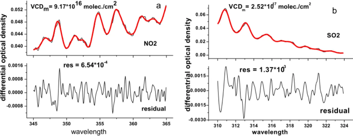
Fig. 2.Example fit for (a) NO2recorded at 10:42 (LT) on 27 November 2010 and(b)SO2at 10:35 (LT) on 29 November 2010 by our mobile

DOAS instrument. Black lines denote the differential optical densities (DODs) of processed measurement spectra. Red lines show the result of the fit. The number given by VCDmis the differential VCD with respect to the Frauenhofer reference spectrum as described in Sect. 2.4.1.

The spectral evaluation applied to each recorded spectrum while the van moves along the measurement route starts with dark current and offset corrections, followed by the divi-sion with a Frauenhofer reference spectrum. Subsequently, a high-pass filter is applied to the logarithm of this ratio to sep-arate the broad and narrow band spectral structures. Differ-ential slant column densities (DSCD, the difference between the slant column density of a measurement spectra and the reference; slant column density, SCD, defined as the concen-tration integrated along the light path), are then obtained by fitting narrow band spectral absorption cross sections to the processed measurement spectra. Figure 2 illustrates such a DOAS fit for NO2 and SO2 using the WinDOAS software

package (Van Roozendael et al., 2001) for mobile DOAS measurement.

During our retrieval process, a spectrum is first selected arbitrarily on the upwind path as the reference spectrum to obtain the concentration distribution trends along the route. The minimum concentration of SO2 and NO2 along each

driving route is then chosen as the Frauenhofer spectra to re-retrieve the measurement spectra. The spectrum with the lowest measurement value for each day is then chosen as the Frauenhofer reference to minimize the effect of potential in-strumental changes on different days.

The wavelength range of 310 nm to 324 nm with three strong absorption peaks is selected for the SO2fit.

Absorp-tion cross secAbsorp-tions of SO2, NO2, HCHO and O3at 293 K are

taken from Bogumil et al. (2003). Apart from the Frauen-hofer reference spectrum, a Ring spectrum is also included in the fit as described in H¨onninger et al. (2004). All ab-sorption cross sections are convoluted with the instrument’s slit function to adapt to the instrument resolution during the fit process. The emission peak from mercury lamp at 334 nm is recorded to yield instrument’s slit function. The synthetic Ring spectrum is generated from the measured Frauenhofer reference spectrum using the DOASIS software

(Kraus, 2006). For the analysis of NO2, the spectral window

of 345 nm to 365 nm is selected, and the cross sections of O4 at 298 K (Greenblatt et al., 1990) and HONO at 298K

(Stutz et al, 2000) are also included, except for NO2, HCHO,

O3at 293 K (Bogumil et al., 2003) and Ring spectrum. The

wavelength calibration is performed using a highly resolved solar spectrum (Kurucz et al., 1984) convoluted by the instru-ment’s slit function. An example for such a spectral fitting is shown in Fig. 2, where the fit residual of NO2(Fig. 2a) and

SO2(Fig. 2b) are 6.54×10−4and 1.37×10−3, respectively,

due to the unknown structures and system noise. The fit un-certainties of retrieved values from these two spectra for NO2

and SO2are about 1.80 and 2.30 %, respectively. For all

mea-sured spectra the fit uncertainties are less than 15 % for NO2

and 20 % for SO2.

The procedure described so far yields differential slant column densities relative to the reference spectrum. The as-sumption by Johansson et al. (2008) and Rivera et al. (2009) that around noon the slant column densities for the zenith viewing direction approximate those of the vertical columns is now adopted. The tropospheric vertical columns obtained from the MAX-DOAS observation at the time the mobile DOAS passes its location (Fig. 1) is used in order to elim-inate the NO2and SO2VCD in the reference. However, this

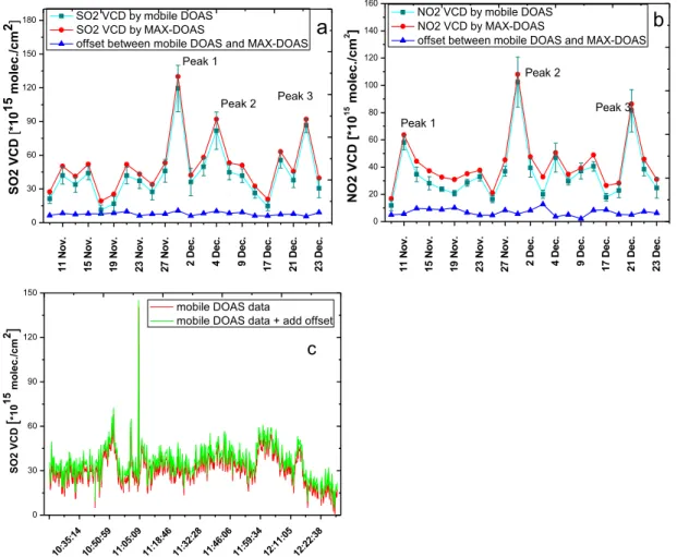
method is based on the assumption that no strong spatial variations exist within the distance represented by the MAX-DOAS measurement (typically several kilometers). The vari-ability of the mobile DOAS VCDs in the form of standard deviation of its values along such a typical distance is shown in Fig. 3a and b for SO2 and NO2, respectively. The

mo-bile DOAS VCDs are averaged for about twenty values from twenty spectra in Fig. 3a and b. Since the integration time of an individual spectrum is 10 s and the average van speed is 70 km h−1_{, this means the van moves about 4 km in the time}

these twenty spectra are taken. In terms of these standard de-viations, for most days no significant variations can be found.

2 2 1 1 N o v . 1 5 N o v . 1 9 N o v . 2 3 N o v . 2 7 N o v . 2 D e c . 4 D e c . 9 D e c . 1 7 D e c . 2 1 D e c . 2 3 D e c . 0 30 60 90 120 150 180 Peak 3 Peak 2 SO2 V C D [ *1 0 15 m ol ec ./ cm

2] _{SO2 VCD by MAX-DOAS}SO2 VCD by mobile DOAS

offset between mobile DOAS and MAX-DOAS

Peak 1

a

15 m

o

lec

./c

m

2 ]

NO2 VCD by mobile DOAS NO2 VCD by MAX-DOAS

offset between mobile DOAS and MAX-DOAS

b

mobile DOAS data

mobile DOAS data + add offset

c

Fig. 3.Offset between MAX-DOAS and mobile DOAS values defined as the difference between these values for the measurement period for SO₂(a)and NO₂(b). The mobile DOAS value represents the average over about twenty spectra data acquired when the mobile DOAS passed the MAX-DOAS location. The MAX-DOAS value is the VCD acquired at the time of the passing by.(c)shows the example for SO2

on 25 November 2010. Red line: original value from mobile DOAS; green line: result after adding the offset. Error bars indicate the standard deviation for the mobile DOAS as described in the text.

Exceptional large variations occur for SO2on 29 November,

and 2 and 4 December, and for NO2on 29 November, and

4 and 21 December. These maybe related to the variations of the emission sources themselves. In general, however, the above assumption of generally small spatial variations ap-pears reasonable to us.

The difference between the MAX-DOAS VCD and the mobile DOAS differential VCD is considered as the “clean-air” background (this difference is called “offset”). The mo-bile DOAS differential VCDs are then converted into abso-lute columns by adding this “offset” to all values along the path.

The retrieval of vertical columns from the MAX-DOAS observations is described by Xu et al. (2010). Differential slant column densities are converted into tropospheric VCDs using tropospheric differential air mass factors (DAMFs)

ac-cording to the following formula: VCDtrop=

DSCDs

DAMF. (1)

The radiative transfer model SCIATRAN (Rozanov et al., 2002) is used to calculate DAMFs under the assumption that aerosol and trace gas profiles are given by constant values below the boundary layer height and exponential profiles above. The height of the boundary layer was on average about 1.5 km during our measurements from the lidar observations. For the radiative transfer calculations, aerosol extinction coefficients within the layer are taken from the lidar, while the NO2 and SO2 mixing ratios are

MAX-DOAS is a potential source of error. We estimated the effect on our retrieval to be less than 5 % by varying the setting of NO2and SO2loading (2.5×1011molec cm−3,

6.25×₁₀11_{molec cm}−3 _{and 1.25}×₁₀12_{molec cm}−3)

within the boundary layer. Another uncertainty lies in the AOD (Aerosol Optical Depth, AOD) obtained from the lidar boundary layer height and extinction coefficients. A sensitivity study for different AODs (0.3, 0.5, 0.8 and 1.1), fixed boundary layer height of 1.5 km and constant NO2

and SO2 concentrations of 1×1012molec cm−3 shows a

resulting change for the NO2and SO2AMFs at 20◦elevation

of less than 10 %.

2.4.2 Emission calculation

The mobile DOAS measurement allows emission from pol-lutant sources to be further quantified for known wind di-rection, wind speed, and car speed. The total SO2and NO2

emissions from a source are determined using the following Eq. (2) (Johansson et al., 2009; Ibrahim et al., 2010): Fluxgas=

X

VCDgas·Vm·Vw⊥·1t , (2) where VCDgasis the vertical column density,Vm is the car

speed,Vw⊥ is the component of wind speed perpendicular to the driving direction, and1t is the time for acquiring one spectrum (i.e., integration time, about 9 s in this study). In this equation, the sum refers to all the measurement spectra along the path.

Assuming additional factors for the partitioning between NO and NO2 and the finite NOx lifetime, mobile DOAS

measurements allow furthermore determining the total NOx

(=NO+NO2)emission (Ibrahim et al., 2010; Shaiganfar et

al., 2011):

FNOx=R·cτ·FluxNO2. (3)

Here,R is ratio of NOxand NO2. This value is considered

to be about 1.38 during daytime with an uncertainty of about 10 % according to the measurement results of Su et al. (2008) in the PRD. The factorcτaccounts for the destruction of

orig-inally emitted NOxon the way to measurement location. It

depends on the wind speed (W) and measurements distance (D) in the following way:

cτ =e

D/W

t _{. (4)}

The NOxlifetime t depends, amongst others, on the ozone

and OH concentrations, as well as meteorological conditions. We here take a value of 5 h (Lin et al., 2010). The resultingcτ

is in the range of 1.10–1.35 assuming an average distance of 9 km from the emission source to the measurement location. We estimate the uncertainty ofcτ due to the uncertainties

of the NOx lifetime, wind speed and distance to be about

10–15 %.

Wind direction and speed are taken from the miniature mobile weather station installed on the van. The car speed,

location, and direction of each segment are from the GPS. The main errors in the estimation of SO2 emission are

un-certainties in the VCD retrieval (including unun-certainties in the DOAS fit of SCDs and errors due to the conversion from SCDs to VCDs) and wind field (including the uncertainties of wind direction and wind speed). Errors of NOxemission

calculations include the uncertainties inR andcτ. We

esti-mate the error caused by approximating VCDs by SCDs with radiative transfer calculations of the zenith AMF to be about 10–15 %. Taking all the above error estimates into account results in an error for our VCD retrieval of less than 20 % and 25 % for NO2 and SO2, respectively. The wind field is

the largest error source not only due to its variation with time and location within the encircled area, but also because of uncertainties of its vertical distribution. The error caused by the wind field is discussed in detail in Sect. 3.2.1.

3 Results and discussion

3.1 Distribution of SO2and NO2around GEA

3.1.1 Identification of emission sources

In this section, the distributions of SO2 and NO2 vertical

columns along the measurement path are analyzed following the results of the mobile DOAS data described in Sect. 2. The possible emission sources are discussed further using these distributions for different wind fields.

Figure 3 shows the resulting MAX-DOAS VCDs dur-ing the measurement period. Figure 3a and b also il-lustrate the mobile DOAS VCDs and the offsets be-tween the two instruments. The average offsets of SO2 and NO2 are 7.83±1.42×1015molec cm−2 and

7.02±_2.41×₁₀15_{molec cm}−2_{, respectively. An example}

result of SO2 after SO2 offset correction on 25 November

is shown in Fig. 3c. Three peaks are also found in Fig. 3a and b. The peaks of SO2(peak 1, peak 2, peak 3) are related

to strong emissions of pollutant sources under the northeast-erly wind. The peaks of NO2(peak 1 and peak 2) on 11 and

29 November are presumably caused by the same pollutant source, but the peak on 21 December (peak 3) may be re-lated to the transport from other regions by the northwesterly wind.

Figure 4a shows the wind direction and wind speed dur-ing the whole experimental period. The wind came mostly from the north and northeast with the exception of 21 and 27 November, 5 and 13 December (southeast direction), 30 November and 21 December (northwest), and 4 and 23 De-cember (east). Average wind speed at ground level ranged from 1 m s−1to 5 m s−1during the measurement period. Ac-cording to the distributions of SO2and NO2around the path,

four types of wind fields are distinguished in our study: north or northeast, southeast, east, and northwest.

2 2 9 N o v . 1 1 N o v . 1 3 N o v . 1 5 N o v . 1 7 N o v . 1 9 N o v . 2 1 N o v . 2 3 N o v . 2 5 N o v . 2 7 N o v . 2 9 N o v . 3 0 N o v . 2 D e c . 3 D e c . 4 D e c . 5 D e c . 7 D e c . 9 D e c . 1 3 D e c . 1 7 D e c . 1 9 D e c . 2 1 D e c . 2 2 D e c . 2 3 D e c . 2 6 D e c . 0 90 180 270 360 N W E S win d s p e e d m/s wind direction wind speed win d d ir e c ti o n d e g N 0 3 6 9 12 a 9 N o v . 1 1 N o v . 1 5 N o v . 1 7 N o v . 1 9 N o v . 2 3 N o v . 2 D e c . 3 D e c . 4 D e c . 1 3 D e c . 1 7 D e c . 1 9 D e c . 2 1 D e c . 2 2 D e c . 0 90 180 270 360 wind d ir e c ti o n d e g N S W N

wind direction @400m wind direction @ surface

E

b

Fig. 4. (a) Time series of average wind direction and wind speed from 10:00 to 13:00 (LT) during the measurement period recorded by our mobile miniature weather station. (b) Compari-son of wind direction at surface and 400 m height. The surface wind fields are from the mobile weather station. The wind field at 400 m is taken from observations at King’s Park (station number: 45004, 114.16◦_{E, 22.31}◦_{N) in Hong Kong (http://weather.uwyo.} edu/upperair/sounding.html).

Typical spatial distributions of SO2 and NO2 vertical

columns around GEA for these four different wind fields are shown in Fig. 5. The maps for SO2 in Fig. 5 show a peak

in the north irrespective of wind direction, suggesting an ad-ditional emission source outside the GEA and north from it. The comparison for wind direction from north/northeast and east versus west further suggests that it is located in the north-east rather than the northwest. No such peak exists for NO2

in the north if the wind is coming from the north, so that we infer a SO2 source (no dominant NO2 emission) lies in the

northeast of GEA (S1 in Fig. 1).

For the southeast wind, downwind peaks are found si-multaneously for SO2 and NO2 in the northwest corner of

our route (Fig. 5b). The corresponding downwind peaks for the reverse wind direction from the northwest are less pro-nounced, and thus sources of NO2and SO2within the

encir-cled measurement area, but closer to the northern measure-ment route, can be identified (S2 in Fig. 1). The location of peaks in the downwind region for the north and northeast wind (Fig. 5a and c) is consistent with this conjecture.

Increased values of NO2appeared for all wind directions

in the southeast/south of the measurement route, especially on 29 November and 4 December. These high column den-sities can most likely be attributed to traffic emissions from

Humen Bridge in the south of GEA (S3 in Fig. 1), the main channel from Shenzhen and Dongguan to Guangzhou. Dur-ing the Asian Games, the Guangzhou government set up a security checkpoint here, which occasionally caused traffic jams that enhanced high NO2concentration.

3.1.2 Comparison with OMI NO2

We compare the results from mobile DOAS with OMI ob-servations in this section in two ways. First, the NO2VCDs

of the mobile DOAS are averaged for all mobile DOAS ob-servations of a given day within one specific ground pixel (113.50◦_E–113.75◦_{E, 22.75}◦_N–23.00◦_{N) and compared to} OMI values within this pixel. Second, in order to explore spatial patterns, all NO2VCDs along the measurement path

of the mobile DOAS are compared to OMI values on the 0.1◦_×0.1◦_{grid, as specified in Sect. 2.3. Mobile DOAS} val-ues were averaged for all measurement days within the pixels of this higher resolved grid.

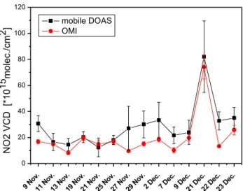
The comparison of NO2 VCDs between the two

instru-ments for the above-ground pixel is shown in Fig. 6. Our mo-bile DOAS values were higher than the OMI values most of the time, especially for the measurements from 27 Novem-ber to 7 DecemNovem-ber. Aside from the averaged value of OMI for large areas and its insensitivity to the near-surface pollu-tant sources, the influence of clouds was also considered and treated as a dominant factor for the OMI and mobile DOAS observations.

Cloud fractions for our 14 days of measurement (Table 1) varied considerably during the measurement period. A cloud fraction of 0.4 was used as threshold to filter both data for comparison. This fraction was exceeded on 21, 27, and 29 November, as well as 7 and 9 December. Figure 7 shows the correlation between the two measurements for cloud fractions smaller than 0.4 for the ground pixel (113.50◦E– 113.75◦_{E, 22.75}◦_N–23.00◦_{N). The correlation coefficient} (R2) is 0.88, indicating that relative changes observed by OMI and mobile DOAS were coinciding.

Although both instruments agree in general, high NO2

113.45 113.50 113.55 113.60 113.65 113.70 22.75

22.80 22.85 22.90 22.95 23.00 23.05 23.10

la

ti

tu

d

e

longitude GEA

SO2

113.45 113.50 113.55 113.60 113.65 113.70 22.75

22.80 22.85 22.90 22.95 23.00 23.05 23.10 NO2

GEA

la

ti

tu

d

e

longitude

a

113.45 113.50 113.55 113.60 113.65 113.70 22.75

22.80 22.85 22.90 22.95 23.00 23.05 23.10 _SO2

la

ti

tu

d

e

longitude GEA

113.45 113.50 113.55 113.60 113.65 113.70 22.75

22.80 22.85 22.90 22.95 23.00 23.05 23.10

b

NO2

GEA

la

ti

tu

d

e

longitude

113.45 113.50 113.55 113.60 113.65 113.70 22.75

22.80 22.85 22.90 22.95 23.00 23.05 23.10 _SO2

GEA

la

ti

tu

d

e

longitude

113.45 113.50 113.55 113.60 113.65 113.70 22.75

22.80 22.85 22.90 22.95 23.00 23.05 23.10

c NO2

GEA

la

ti

tu

d

e

longitude

113.45 113.50 113.55 113.60 113.65 113.70 22.75

22.80 22.85 22.90 22.95 23.00 23.05 23.10 _SO2

GEA

la

ti

tu

d

e

longitude

113.45 113.50 113.55 113.60 113.65 113.70

22.75 22.80 22.85 22.90 22.95 23.00 23.05 23.10

GEA

NO2

la

ti

tu

d

e

longitude

0 6.0 12 18 24 30 *1016

d

– –

Fig. 5.Examples of SO2and NO2vertical columns (units: molec cm−2)along the measurement path of the mobile DOAS for four typical

wind directions:(a)northeast/north on 29 November,(b)southeast on 5 December,(c)east on 4 December, and(d)northwest 30 November. Arrows indicate the average wind direction.

2 2

9 N ov.

11 N ov.

13 N ov.

19 N ov.

21 N ov.

25 N ov.

27 N ov.

29 N ov.

2 D ec.

7 D ec.

9 D ec.

21 D ec.

22 D ec.

23 D ec.

0 20 40 60 80 100 120

mobile DOAS OMI

NO2 VCD

[*

10

15

m

olec./

cm

2 ]

– –

Fig. 6.Time series of NO2VCDs measured by mobile DOAS (black

symbols) and OMI (red symbols) for the satellite ground pixel given by the coordinates (113.50◦E–113.75◦E, 22.75◦N–23.00◦N). The measurement time of the mobile DOAS within this area is from about 11:00 to 12:00 (LT). The bars show the standard deviations of OMI and mobile DOAS as described in the text.

0 20 40 60 80 100 120 0

20 40 60 80 100 120

m

ob

ile DOAS

NO2

VC

D

[*

10

15

m

ole

c./cm

2 ]

OMI NO2 VCD [*1015molec./cm2]

y=0.98x+8.64 R2=0.88

1:1

– –



–

Fig. 7. Correlation between the OMI and mobile DOAS NO₂ VCDs after cloud filtering for the satellite ground pixel (113.50◦E– 113.75◦E, 22.75◦N–23.00◦N).

observations of NO2in general show little variation between

11:00 and 13:00 LT, see Fig. 8 (a similar observation was made for Hong Kong in Chan et al., 2012), we conclude that for our case the effect of the daily NO2cycle between 11:00

and 13:00 LT is of minor importance for this comparison of mobile and satellite measurements.

We now compare spatial patterns as described at the begin-ning of this section. Figure 9 shows that both mobile DOAS and OMI captured the high NO2VCDs in the northern and

southern part of the mobile DOAS route (in the northern part due to industrial emissions, in the southern part due to vehi-cle emissions from the Humen Bridge), as well as low VCDs

Table 1.Cloud fraction for the 14 days of measurement. Italic text represents the cloud fraction<0.4. Bold text represents the cloud fraction>0.4. Cloud fractions are taken from the OMI data product.

Date Cloud fraction

9 Nov 0.24

11 Nov 0.20

13 Nov 0.37

19 Nov 0.11

25 Nov 0.15

2 Dec 0.25

21 Dec 0.18

22 Dec 0.06

23 Dec 0.01

21 Nov 0.66 27 Nov 0.56 29 Nov 0.41 7 Dec 0.63 9 Dec 0.50

– –

00:00 04:00 08:00 12:00 16:00 20:00 24:00 30

40 50 60 70 80 90

N

O2

a

v

e

ra

g

e

c

o

n

c

e

n

tr

a

ti

o

n



g

/m

3

Local Time NO2 concentration by LP-DOAS

– –

Fig. 8.Mean daily NO2cycle of the LP-DOAS from 11

Novem-ber to 25 DecemNovem-ber 2010, at Guangzhou University Town site. The black hatched region indicates the OMI overpass time for Guangzhou. The red hatched region indicates the time when the mobile DOAS traverses the area of the satellite ground pixel (113.50◦E–113.75◦E, 22.75◦N–23.00◦N).

in the western part (white circles in Fig. 9). The correla-tion analysis for these three areas (indicated by white cir-cles in Fig. 9) is shown in Fig. 10. The correlation coefficient (R2)is 0.72, suggesting that both observations indeed agree reasonably well. However, no such agreement can be found when all grid cells are taken into account. One reason for the lack of correlation might be that data are compared for the same location, but not the same time. Comparing two val-ues for times when the diurnal variation cannot be neglected inevitably leads to mismatch between both data sets. Accord-ing to Fig. 8, strong diurnal changes of NO2occur between

10:00 and 11:00 LT. During this time, mobile DOAS

×

Fig. 9. Comparison of NO2 VCD patterns measured by mobile

DOAS and OMI (ground pixel: 113.25◦E–113.75◦E, 22.75◦N– 23.25◦N) during the whole measurement period (9 November to 23 December 2010). The color-coded circle indicates the mobile DOAS observations. The white circles in the northern and south-ern part show particularly high NO2values captured by both

instru-ments. The white circle in the western part contains low NO₂values for both instruments. The grid resolution is 0.1◦×0.1◦.

tions were carried out in the eastern part of the GEA. Lacking further data from longer measurements or models, we do not attempt a correction of this mismatch, but notice that it might have significant influence even for the relatively limited time of our mobile measurements.

3.2 Estimation of SO2and NOxemissions

3.2.1 Emission of SO2and NOxfrom GEA

As a key component in the estimation of SO2and NOx

emis-sions, wind fields can be the source of large errors. Wind fields are generally used to estimate emissions about 400 m above ground level (according to the stack height of a power plant and the height of an elevated plume as discussed by Mellqvist et al., 2007). A wind profile radar could provide highly accurate data, but was not available for our measure-ments. Wind data from our mobile weather station are used instead. To minimize the error caused by the influence of sur-face processes on the wind field, measurement days with rel-atively constant wind field from ground to 400 m height are selected to estimate emissions. Figure 4b compares the wind direction at 400 m height to the surface from 9 November to 22 December. The wind field at 400 m is taken from ob-servations at Kings Park (station number: 45004, 114.16◦_E, 22.31◦_{N) in Hong Kong, about 80 km southeast of GEA} (http://weather.uwyo.edu/upperair/sounding.html). With few exceptions, Fig. 4b illustrates that the wind direction at both

16 17 18 19 20 21 22

18 19 20 21 22

R2=0.72 y=0.46x+11.10

OMI

N

O2

VCD

[*1

0

15

molec

./

c

m

2 ]

mobile DOAS NO2 VCD [*1015molec./cm2]

Fig. 10.Correlation analysis of OMI and mobile DOAS NO2VCDs

for the three areas (white circles) in Fig. 9. Values are averaged over the whole measurement period for both instruments.

altitudes generally agree, with a relative deviation of∼30◦_. Based on this variation, we estimate the error of our emis-sions due to change of wind direction with height to be 20 %. While the wind direction in the higher atmosphere might vary little over a relatively small area, the wind speed can change significantly for different locations. We do not take into ac-count differences in the wind speed profiles between differ-ent locations. Instead, the ratio of wind speeds at 400 m to that at ground level was estimated to be 1.2–1.3 according to the national standard (GB/T 3840-91) from the environmen-tal protection agency of China (Ministry of Environmenenvironmen-tal Protection of the People’s Republic of China, 1992). So we simply use the wind speed at ground to estimate emission errors caused by uncertainties in the wind speed profile and arrive at a value of about 20–30 %.

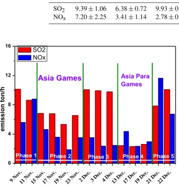
Total emissions of SO2and NOxfrom the encircled GEA

area obtained from Eq. (2) are shown in Fig. 11 for 14 days with a fractional cloud cover lower than 0.4 and a constant wind field. The entire measurement period is divided into five phases: before the Asian Games (9 and 11 November, phase 1), during the Asian Games (15, 17, 19, and 23 Novem-ber, phase 2), the time between the Asian Games and the Asian Para Games (2, 3, and 4 December, phase 3), during the Asian Para Games (13, 17, and 19 December, phase 4), and after the games (21 and 22 December, phase 5). SO2

emissions varied strongly between the different phases (by a factor of 5), where the lower and lowest emissions occurred during the Asian Games and Asian Para Games, respectively. A clear pattern for NOxemissions was not found, although

these emissions decreased at the beginning of the games and increased again after their end.

The reduced emission of SO2during the Asian Games and

Asian Para Games could be caused mainly by the pollution control strategy of the local environmental protection agency.

2 2

Table 2.SO2and NOxemissions as measured by our mobile DOAS for the different phases described in the text.

Emission ton h−1

Phase 1 Phase 2 Phase 3 Phase 4 Phase 5 Phase 1+3+5

SO2 9.39±1.06 6.38±0.72 9.93±0.15 2.45±0.15 8.97±1.58 9.50±0.90

NOx 7.20±2.25 3.41±1.14 2.78±0.64 3.22±1.04 9.19±3.47 5.87±3.46

9 N

ov.

11 N

ov.

15 N

ov.

17 N

ov.

19 N

ov.

23 N

ov.

2 D

ec.

3 D

ec.

4 D

ec.

13 D

ec.

17 D

ec.

19 D

ec.

21 D

ec.

22 D

ec.

0 4 8 12 16

Phase 5 Phase 4

e

miss

io

n

t

o

n

/h

SO2 NOx

Phase 3 Phase 2

Asia Para Games Asia Games

Phase 1

Fig. 11.SO2 and NOx emissions estimated from mobile DOAS

measurements between 10:00 to 13:00 (LT). Green lines indicate the beginning and end of the Asian and Asian Para Games.

Meteorological conditions also play an important role for emissions from GEA. Persistent rainfall from 10 to 12 De-cember and again from 14 to 16 DeDe-cember helped to remove air pollutants, thereby decreasing emissions from GEA dur-ing the Asian Para Games. Table 2 summarizes the average SO2 emission for the different phases of the measurement

period. For times outside the games (phases 1, 3, and 5), SO2

emission was estimated to be 9.50 tons per hour (approxi-mately 83.2×103 tons per year), which is consistent with the value of 84.60×103tons per year from the emission in-ventory (Guangzhou Municipality State of the Environment, 2010). On the other hand, the average NOx emission for

this time was estimated to be 5.87 tons per hour. During the games (including phases 2 and 4) the emissions of SO2and

NOx from GEA were reduced by 53.50 % and 43.50 %,

re-spectively, compared with the time outside the games (in-cluding phases 1, 3, and 5).

Errors in the calculation of emissions are due to errors in the VCD retrieval, wind field, and car speed. The total er-ror in the VCD retrieval was estimated to be less than 20 % for NO2and 25 % for SO2. The error of the car speed was

about 1 % according to the GPS. The errors caused by wind direction and wind speed were about 20 % and 20–30 %, re-spectively, or about 30–35 % together. The total error for the estimate of SO2emissions amounts to about 35–40 %.

Addi-tional uncertainties caused byRandcτof 10 % and 10–15 %,

result in a total error of NOxemissions of about 40–45 %. 3.2.2 Influence of SO2emissions from the GEA on the

downwind region

Knowledge of emissions and transport from large area sources is crucial for the control and management of lo-cal environment problems. Guangzhou University Town (23.05◦_{N, 113.37}◦_{E) hosted numerous events during the} Asian Games, which raised issues on the air quality of the town. According to the geographical relationship between GEA and Guangzhou University Town from Fig. 1, the pol-lutants from GEA can diffuse to Guangzhou University Town when the wind direction is southeast. The SO2concentration

in Guangzhou University Town is expected to increase due to the contribution of GEA emission. SO2is selected as the

tracer gas because it originates from industrial emissions, un-like NO2which is still affected by local vehicle emissions. To

investigate how emissions from GEA affect Guangzhou Uni-versity Town for southeasterly winds, a long-path DOAS in-strument is set up there to monitor possible downwind trans-port of SO2.

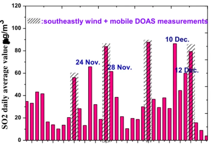
The paths of air masses for southeasterly wind on 21 and 27 November, and 5 and 13 December are shown in Fig. 12. On these days, the wind traversed GEA and the SO2

concentrations measured downwind at the University Town monitoring site by our long-path instrument were signifi-cantly higher, as illustrated in Fig. 13 (shaded box). Sim-ilar phenomena can be observed on 24 and 28 November and 10 and 12 December in Fig. 13, when the wind was also coming from the southeast. The average SO2

concen-trations for southeasterly and non-southeasterly winds mea-sured by the long-path DOAS at the downwind location are 72.55±13.06 µg m−3_{and 24.58±11.72 µg m}−3_,

respec-tively. Daily averages of SO2are enhanced by a factor 3 when

air masses traversed GEA, compared to days when the wind came from other directions. Therefore, GEA is concluded to be a major contributor to SO2 pollution in the Guangzhou

University Town area.

4 Conclusions

a

b

c

_d

Fig. 12.Backward wind trajectories for the 200 m (red), 400 m (blue), and 800 m (green) heights at the Guangzhou University Town mon-itoring site from the NOAA HYSPLIT model (http://www.arl.noaa.gov/index.php) on 21(a)and 27(b)November, and 5(c)and 13(d)

December. The star indicates the Guangzhou University Town monitoring site, the black box the measurement area of the mobile DOAS measurement.

to investigate the spatial and temporal distributions of SO2

and NO2around and emissions from GEA during the Asian

Games period.

A MAX-DOAS instrument at a fixed location concur-rently measured estimates of absolute vertical columns for NO2and SO2of the mobile DOAS measurements. The

av-erage offsets of SO2 and NO2 between the mobile DOAS

and MAX-DOAS were 7.83±1.42×1015_{molec cm}−2 _and

7.02±2.41×1015_{molec cm}−2_{, respectively.}

Distributions of SO2and NO2vertical columns were

ob-tained with help of the mobile DOAS system. High SO2

values appeared in the northeast and northwest of our mea-surement path under north and southeast wind fields, respec-tively. High NO2values were found in the north and

south-east of the measurement path with higher variability due to

2 2

13 N ov.

15 N ov.

17 N ov.

19 N ov.

21 N ov.

23 N ov.

25 N ov.

27 N ov.

29 N ov.

1 D ec.

3 D ec.

5 D ec.

7 D ec.

9 D ec.

11 D ec.

13 D ec.

15 D ec.

0 20 40 60 80 100 120

12 Dec. 10 Dec.

28 Nov. 24 Nov.

SO2 d

aily aver

age value



g/

m

3 :southeastly wind + mobile DOAS measurements

Fig. 13.Daily average SO₂concentrations measured by long-path DOAS at the Guangzhou University Town site. The shaded days indicate days when the wind came from the southeast and mobile DOAS measurements were conducted. For days with similar wind situations on 24 and 28 November and 10 and 12 December, we could not conduct mobile DOAS measurements due to vehicle lim-itation.

varying traffic emissions. Possible emission sources were de-termined to explain these distributions using the information from different wind fields. Pollutant sources in the northeast of GEA, outside the closed measurement route and sources in the north, within the area encircled, were also identified. Our NO2 vertical columns were compared with OMI data

and were found to be similar in spatial patterns. The correla-tion coefficient (R2)of the vertical columns after cloud filter-ing was 0.88 within a specific ground pixel, but the absolute values measured by our mobile DOAS were mostly higher than the OMI data. SO2and NOxemissions from the GEA

during the Asian Games period were also calculated. Lower and lowest emissions of SO2were found to occur during the

Asian Games and Asian Para Games, respectively. Outside the Asian Games period, the average emission of SO2was

es-timated to be 9.50±0.90 tons per hour (83.2 thousand tons per year), which is consistent with the value of 84.6 thou-sand tons per year from a local emission inventory. In com-parison, the average emission of NOx was estimated to be

5.87±3.46 tons per hour. During the games, the emissions of SO2and NOxwere reduced by 53.50 % and 43.50 %,

re-spectively. The error of total emissions was estimated to be about 40–45 % for NOx and 35–40 % for SO2. Using

LP-DOAS measurements at the Guangzhou University Town, emissions from GEA were found to have a distinct impact on air pollution in this area depending on the wind direction. SO2concentrations were found to be about three times larger

during our measurements when air masses crossed GEA.

Acknowledgements. The authors would like to thank the

Guangzhou Environmental Center for supporting the experiment. We also want to thank our two drivers, Shaoli Wang and Zong-mao Xu, whose skillful driving ensured that the experiment could be carried out successfully and safely. This work was also made possible by the support of special research funding for the public industry sponsored by Ministry of Environmental Protection of PRC (Grant No: 201109007), the National Natural Science Foundation of China 40905010, 41275038 and the Anhui Province Natural Science Foundation of China 1308085QF124.

Edited by: J. Stutz

References

Bogumil, K., Orphal, J., Homann, T., Voigt, S., Spietz, P., Fleis-chmann, O. C., Vogel, A., Hartmann,M., Kromminga, H., Bovensmann, H., Frerick, J., and Burrows, J. P.: Measurements of molecular absorption spectra with the SCIAMACHY pre-flight model: instrument characterization and reference data for atmospheric remote-sensing in the 230–2380 nm region, J. Pho-toch. Photobio. A, 157, 167–184, 2003.

Bucsela, E., Celarier, E., Wenig, M., Gleason, J., Veefkind, P., Boersma, K., and Brinksma, E.: Algorithm for NO₂vertical col-umn retrieval from the Ozone Monitoring Instrument, IEEE T. Geosci. Remote, 44, 1245–1258, 2006.

Cao, J. J., Lee, S. C., Ho, K. F., Zou, S. C., Fung, K., Li, Y., Watson, J. G., and Chow, J. C.: Spatial and seasonal variations of atmo-spheric organic carbon and elemental carbon in Pearl River Delta Region, China, Atmos. Environ., 38, 4447–4456, 2004. Chan, K. L., P¨ohler, D., Kuhlmann, G., Hartl, A., Platt, U., and

Wenig, M. O.: NO2measurements in Hong Kong using LED

based long path differential optical absorption spectroscopy, At-mos. Meas. Tech., 5, 901–912, doi:10.5194/amt-5-901-2012, 2012.

Chen, Z. Y., Liu, W. Q., Zhang, Y. J., He, J. F., and Ruan, J.: Mixing layer height and meteorological measurements in Hefei China during the total solar eclipse of 22 July, 2009, Opt. Laser Tech-nol., 43, 50–54, 2011.

Dix, B., Brenninkmeijer, C. A. M., Frieß, U., Wagner, T., and Platt, U.: Airborne multi-axis DOAS measurements of atmospheric trace gases on CARIBIC long-distance flights, Atmos. Meas. Tech., 2, 639–652, doi:10.5194/amt-2-639-2009, 2009. Edner, H., Ragnarson, P., Svanberg, S., Wallinder, E., Ferrara, R.,

Cioni, R., Raco, B., and Taddeucci, G.: Total fluxes of sulfur dioxide from the Italian volcanoes Etna, Stromboli, and Vulcano measured by differential absorption lidar and passive differential optical absorption spectroscopy, J. Geophys. Res., 99, 18827– 18838, 1994.

Finlayson-Pitts, B. J. and Pitts, J. N.: Chemistry of the Upper and Lower Atmosphere: Theory, Experiments, and Applications, Academic Press, San Diego, USA, 1999.

Galle, B., Oppenheimer, C., Geyer, A., McGonigle, A. J. S., Ed-monds, M., and Horrocks, L.: A miniaturised ultraviolet spec-trometer for remote sensing of SO2fluxes: a new tool for volcano

surveillance, J. Volcanol. Geoth. Res., 119, 241–254, 2003. Greenblatt, G. D., Orlando, J. J., Burkholder, J. B., and

330 nm and 1140 nm, J. Geophys. Res.-Atmos., 95, 18577– 18582, doi:10.1029/JD095iD11p18577, 1990.

Guangzhou Environmental Protection, Guangzhou Municipality State of the Environment, available at: http://www.gzepb.gov.cn/ zwgk/hjgb/201106/t2011060766789.htm, (last access: January 2013), 2010.

He, M., Zheng, J. Y., Yin, S. S., and Zhang, Y. Y.: Trends, temporal and spatial characteristics, and uncertainties in biomass burning emissions in the Pearl River Delta, China, Atmos. Environ., 45, 4051–4059, 2011.

Heue, K.-P., Brenninkmeijer, C. A. M., Baker, A. K., Rauthe-Sch¨och, A., Walter, D., Wagner, T., H¨ormann, C., Sihler, H., Dix, B., Frieß, U., Platt, U., Martinsson, B. G., van Velthoven, P. F. J., Zahn, A., and Ebinghaus, R.: SO2 and BrO

observa-tion in the plume of the Eyjafjallaj¨okull volcano 2010: CARIBIC and GOME-2 retrievals, Atmos. Chem. Phys., 11, 2973–2989, doi:10.5194/acp-11-2973-2011, 2011.

H¨onninger, G., von Friedeburg, C., and Platt, U.: Multi axis dif-ferential optical absorption spectroscopy (MAX-DOAS), Atmos. Chem. Phys., 4, 231–254, doi:10.5194/acp-4-231-2004, 2004. Ibrahim, O., Shaiganfar, R., Sinreich, R., Stein, T., Platt, U., and

Wagner, T.: Car MAX-DOAS measurements around entire cities: quantification of NOxemissions from the cities of Mannheim

and Ludwigshafen (Germany), Atmos. Meas. Tech., 3, 709–721, doi:10.5194/amt-3-709-2010, 2010.

Johansson, M., Galle, B., Yu, T., Tang, L., Chen, D. L., Li, H. J., Li, J. X., and Zhang, Y.: Quantification of total emission of air pol-lutants from Beijing using mobile mini-DOAS, Atmos. Environ., 42, 6926–6933, 2008.

Johansson, M., Rivera, C., de Foy, B., Lei, W., Song, J., Zhang, Y., Galle, B., and Molina, L.: Mobile mini-DOAS measurement of the outflow of NO₂and HCHO from Mexico City, Atmos. Chem. Phys., 9, 5647–5653, doi:10.5194/acp-9-5647-2009, 2009. Kneizys, F. X., Shettle, E. P., Abreu, L. W., Chetwynd, J. H., and

Anderson, G. P.: Users Guide to LOWTRAN7, Air Force Geo-physics Laboratory, Hanscom AFB, MA, USA, 1988.

Kraus, S.: DOASIS, A Framework Design for DOAS, PhD-thesis, University of Mannheim, Shaker Verlag, Heidelberg, Germany, 2006.

Kurucz, R. L., Furenlid, I., Brault, J., and Testerman, L.: Solar flux atlas from 296 nm to 1300 nm, National Solar Observatory Atlas No. 1, Office of University publisher, Harvard University, Cam-bridge, 1984.

Levelt, P. F., van den Oord, G. H. J., and Dobber, M. R.: The ozone monitoring instrument, IEEE T. Geosci. Remote, 44, 1093–1101, 2006.

Li, A., Liu, C., Xie, P. H., Liu, J. G., Qin, M., Dou, K., Fang, W., and Liu, W. Q.: Monitoring of SO2emissions from

indus-try by passive DOAS, Proc. SPIE, 5832, 0277-786X/05/$15, 10, doi:10.1117/12.619651, 2005.

Li, A., Xie, P. H., and Liu, W. Q.: Monitoring of total emission vol-ume from pollution sources based on passive differential optical absorption spectroscopy, Acta Opt. Sin., 27, 1537–1542, 2007a. Li, A., Xie P. H., Liu, C., Liu J. G., and Liu W. Q.: A scanning

multi-axis differential optical absorption spectroscopy system for measurement of tropospheric NO2in Beijing, Chin. Phys. Lett.,

24, 2859–2862, 2007b.

Lin, J.-T., McElroy, M. B., and Boersma, K. F.: Constraint of anthropogenic NOxemissions in China from different sectors:

a new methodology using multiple satellite retrievals, Atmos. Chem. Phys., 10, 63–78, doi:10.5194/acp-10-63-2010, 2010. Louisa, J. K., Roland, J. L., John, J. R., and Paul, S. M.:

Compari-son of OMI and ground-based in situ and MAX-DOAS measure-ments of tropospheric nitrogen dioxide in an urban area, J. Geo-phys. Res., 113, D16S39, doi:10.1029/2007JD009168, 2008. Melamed, M. L., Basaldud, R., Steinbrecher, R., Emeis, S.,

Ru´ız-Su´arez, L. G., and Grutter, M.: Detection of pollution trans-port events southeast of Mexico City using ground-based visible spectroscopy measurements of nitrogen dioxide, Atmos. Chem. Phys., 9, 4827–4840, doi:10.5194/acp-9-4827-2009, 2009. Mellqvist, J., Samuelsson, J., and Rivera, C.: Measurements of

in-dustrial emissions of VOCs, NH3, SO2and NO2in Texas using

the solar occultation flux method and mobile DOAS, Final Re-port HARC Project H-53, Radio and Space Science Chalmers University of Technology, Goteborg, Sweden, 2007.

Ministry of Environmental Protection of the People’s Republic of China: Technical methods for making local emission standards of air pollutants (GB/T 3840-91), available at: http://kjs.mep.gov. cn/hjbhbz/bzwb/other/qt/199206/t19920601 67580.htm, 1992 Platt, U. and Stutz, J.: Differential Optical Absorption

Spec-troscopy: Principles and Applications, Springer, Heidelberg, Germany, 2008.

Qin, M., Xie, P. H., Liu, W. Q., Li, A., Dou, K., Fang,W., Liu, H. G., and Zhang, W. J.: Observation of atmospheric nitrous acid with DOAS in Beijing, J. Environ. Sci.-China, 18, 69–75, 2006. Rivera, C., Sosa, G., W¨ohrnschimmel, H., de Foy, B., Johansson,

M., and Galle, B.: Tula industrial complex (Mexico) emissions of SO2and NO2during the MCMA 2006 field campaign using a

mobile mini-DOAS system, Atmos. Chem. Phys., 9, 6351–6361, doi:10.5194/acp-9-6351-2009, 2009.

Rozanov, V. V., Buchwitz, M., Eichmann, K. U., de Beek, R., and Burrows, J. P.: Sciatran – a new radiative transfer model for geophysical applications in the 240–2400 nm spectral region: the pseudo-spherical version, Adv. Space Res., 29, 1831–1835, 2002.

Shaiganfar, R., Beirle, S., Sharma, M., Chauhan, A., Singh, R. P., and Wagner, T.: Estimation of NOx emissions from Delhi

using Car MAX-DOAS observations and comparison with OMI satellite data, Atmos. Chem. Phys., 11, 10871–10887, doi:10.5194/acp-11-10871-2011, 2011.

Sluis, W. W., Allaart, M. A. F., Piters, A. J. M., and Gast, L. F. L.: The development of a nitrogen dioxide sonde, Atmos. Meas. Tech., 3, 1753–1762, doi:10.5194/amt-3-1753-2010, 2010. Stutz, J., Kim, E. S., Platt, U., Bruno, P., Perrino, C., and Febo, A.:

UV-visible absorption cross sections of nitrous acid, J. Geophys. Res-Atmos., 15, 14585–14592, 2000.

Su, H., Cheng, Y. F., Cheng, P., Zhang Y. H., Dong, S. F., Zeng, L. M., Wang, X. S., Slanina, J., Shao, M., and Wiedensohler, A., Observation of nighttime nitrous acid (HONO) formation at a non-urban site during PRIDE-PRD2004 in China, Atmos. Envi-ron., 42, 6219–6232, 2008.

Takashima, H., Irie, H., Kanaya, Y., and Akimoto, H.: Enhanced NO2at Okinawa Island, Japan caused by rapid air-mass transport

from China as observed by MAX-DOAS, Atmos. Environ., 45, 2593–2597, 2011.

US government printing office: US Standard Atmosphere, 1976, Washington, DC, October 1976.

2 2

Van Roozendael, C. F.: WinDOAS 2.1 Software User Manual, IASB/BIRA, Brussel, Belgium, 2001.

Wagner, T., Ibrahim, O., Shaiganfar, R., and Platt, U.: Mobile MAX-DOAS observations of tropospheric trace gases, Atmos. Meas. Tech., 3, 129–140, doi:10.5194/amt-3-129-2010, 2010. Wang, W., Ren, L. H., Zhang, Y. H., Chen, J. H., Liu, H. J., Bao,

L. F., Fan, S. J., and Tang, D.: Aircraft measurements of gaseous pollutants and particulate matter over Pearl River Delta in China, Atmos. Environ., 42, 6187–6202, 2008.

Wenig, M. O., Cede, A. M., Bucsela, E. J., Celarier, E. A., Boersma, K. F., Veefkind, J. P., Brinksma, E. J., Gleason, J. F., and Her-man, J. R.: Validation of OMI tropospheric NO2 column

den-sities using direct-sun mode Brewer measurements at NASA Goddard Space Flight Center, J. Geophys. Res., 133, D16S45, doi:10.1029/2007JD008988, 2008.

World Health Organization: WHO Air quality guidelines for partic-ulate matter, ozone, nitrogen dioxide and sulfur dioxide Global update 2005 summary of risk assessment, Geneva, Switzerland, 2006.

Wu, F. C., Xie, P. H., Li, A., Si, F. Q., Wang, Y., and Liu, W. Q.: Correction of the impact of multi scattering on NO2

emis-sion flux during the pollutants source measurement by mobile differential optical absorption spectroscopy, Acta Optica Sinica, 31, 1101003-1–1101003-6, doi:10.3788/AOS201131.1101003, 2011.

Xu, J., Xie, P. H., Si, F. Q., Dou, K., Li, A., Liu, Y., and Liu, W. Q.: Retrieval of tropospheric NO₂by multi axis differential op-tical absorption spectroscopy, Spectrosc. Spect. Anal., 30, 2464– 2469, 2010.

Zhang, Q., David, G. S., He, K. B., Wang, Y. X., Richter, A., Bur-rows, J. P., Uno, I., Jang, C. J., Chen, D., Yao, Z. L., and Lei, Y.: NOxemission trends for China, 1995–2004: the view from the

ground and the view from space, J. Geophys. Res., 112, D22306, doi:10.1029/2007JD008684, 2007.

Zhang, Y. H., Hu, M., Zhong, L. J., Wiedensohler, A., Liu, S. C., Andreae, M. O., Wang, W., and Fang, S. J.: Regional integrated experiments on air quality over Pearl River Delta 2004 (PRIDE-PRD2004): overview, Atmos. Environ., 42, 6157–6173, 2008a. Zhang, Y. H., Hu, M., and Wiedensohler, A.: The special issue on

PRIDE-PRD 2004 campaign, Atmos. Environ., 42, 6155–6156, 2008b.