Reasoning in Reference Games:
Individual-vs. Population-Level Probabilistic Modeling
Michael Franke1*, Judith Degen2
1Department of Linguistics, University of Tübingen, Wilhelmstrasse 19, 72072 Tübingen, Germany, 2Department of Psychology, Stanford University, 450 Serra Mall, Stanford, CA 94305, United States of America
Abstract
Recent advances in probabilistic pragmatics have achieved considerable success in model-ing speakers’and listeners’pragmatic reasoning as probabilistic inference. However, these models are usually applied to population-level data, and so implicitly suggest a homoge-neous population without individual differences. Here we investigate potential individual dif-ferences in Theory-of-Mind related depth of pragmatic reasoning in so-calledreference gamesthat require drawing ad hoc Quantity implicatures of varying complexity. We show by Bayesian model comparison that a model that assumes a heterogenous population is a bet-ter predictor of our data, especially for comprehension. We discuss the implications for the treatment of individual differences in probabilistic models of language use.
Introduction
When Jones complains“I hurt my finger”we are inclined to believe that he is not referring to his thumb, at least much more than when Smith complains“I hurt my toe”we are inclined to believe that he is not referring to his big toe [1,2]. That a particular mention of“finger”is understood as“a finger other than a thumb”is not a matter of semantic meaning, because most humans have ten fingers and no additional thumbs. Instead, the pragmatic inference that Jones is is not referring to his thumb arises, according to standard pragmatic theory, because the wordthumbis a short and salient alternative expression that Jones would likely have used if indeed he meant to refer to his thumb, because that would have been an easy and natural way to increase the information content of his utterance. In contrast, the expressionbig toeis not equally readily at hand for Smith, and so the pragmatic inference that Smith has not hurt his big toe is hampered, if it goes through at all.
The influential approach of philosopher Paul Grice [3] tries to explain pragmatic reasoning patterns like the above as the concomitant of regularities of language use, which in turn he described in terms of certain rules of conduct for cooperative speakers, the so-called Maxims of Conversation. One of these is the Maxim of Quantity, which requires, roughly put, that speak-ers be maximally (but not redundantly) informative given the current purpose of convspeak-ersation. Pragmatic inferences, amongst them so-called Quantity implicatures like the inference from
a11111
OPEN ACCESS
Citation:Franke M, Degen J (2016) Reasoning in Reference Games: Individual- vs. Population-Level Probabilistic Modeling. PLoS ONE 11(5): e0154854. doi:10.1371/journal.pone.0154854
Editor:Philip Allen, University of Akron, UNITED STATES
Received:December 3, 2015
Accepted:April 20, 2016
Published:May 5, 2016
Copyright:© 2016 Franke, Degen. This is an open access article distributed under the terms of the Creative Commons Attribution License, which permits unrestricted use, distribution, and reproduction in any medium, provided the original author and source are credited.
Data Availability Statement:All relevant data are within the paper and its Supporting Information files.
“finger”to“not thumb,”can be explained by the assumption that listeners believe that speakers (by and large) behave in accordance with Grice’s speaker rules. Modern linguists and psycholo-gists like to preserve Grice’s main ideas, while acknowledging that pragmatics is an uncertain, non-deterministic affair: computing a speaker’s intended meaning requires integrating multi-ple contextual cues in a limited amount of time, with possibly a substantial amount of uncer-tainty about relevant contextual parameters like the speaker’s knowledge state or her
preferences over and awareness of linguistic alternatives [4]. The resulting picture is that infer-ence patterns like Quantity implicatures are typically observed in the population as relatively robust, but probabilistic trends [5–12].
Probabilistic pragmaticsis a recent attempt to combine the Gricean approach with the desire to explain complex and contextually-variable empirical data [4]. Probabilistic models have been given for a variety of phenomena, including reasoning about referring expressions [10,
12–15], knowledge implicatures [7], non-literal interpretation [16,17], vague gradable adjec-tives [18,19], syllogistic reasoning [20], or the use of quantifiers [21]. Though different in detail, these models share key ideas. For one, most models include probabilistic versions of Gri-cean speakers and GriGri-cean listeners. For another, model predictions are usually assessed based onpopulation-level datafrom suitable experimental tasks. That is, the data to be explained by a given model are obtained by averaging over the answers of all participants.
Here, we would like to extend probabilistic modeling of pragmatic language use to acknowl-edge potential individual-level differences. One general reason for doing so is that it is well known that what best describes a population’s average behavior need not necessarily be a good description of the behavior of the individuals that comprise the population [22–24]. Another reason specific to pragmatics is that there is evidence in the psycholinguistic literature that lis-teners track speaker-specific (i.e., individual-level) features of their interlocutors, including pragmatic features like the propensity towards over- or under-informativeness [25,26]. In order to bring probabilistic pragmatics closer towards modeling real speaker/listener behavior, this type of evidence suggests that it is vital to incorporate the possibility of individual differ-ences. Moreover, experimental results indicate restrictions on the depth of Theory-of-Mind (ToM) reasoning capacities in strategic situations (reasoning about the beliefs of agentiabout the beliefs of agentj. . .) [27–29]. Probabilistic pragmatics models typically assume that Gricean speakers are level-1 ToM-reasoners, in the sense that speaker models consider listeners to be literal interpreters who do not themselves reason about the speaker’s behavior, beliefs or desires. Similarly, Gricean listeners are assumed to be level-2 ToM-reasoners, in the sense that they consider speakers to be the aforementioned level-1 ToM-reasoners. But since like-minded game-theoretic models also consider other possible reasoning types [30–33], it becomes an empirical question which of these types are credible in the light of experimental data, and a technical challenge how to design a formal model of probabilistic pragmatic reasoning that can accommodate potential individual-level differences.
In order to address these issues, we take a data-oriented approach that infers (probabilisti-cally) a language user’s likely reasoning depth from their empirically observed behavior. We formulate models of different complexity: one that assumes a homogeneous population of Gri-cean speakers and listeners, and one that assumes a heterogeneous population with varying proportions of pragmatic reasoning types inspired by game-theoretic approaches. We assess these models, using Bayesian model comparison [34–36], based on experimental data.
The motivation for this Bayesian approach is that it naturally weighs a model’s complexity in determining its quality. This is particularly important for our case, since we are comparing a simpler model (homogeneous population) to a more complex one (heterogeneous population) with equal numbers of free parameters (see below). The complex heterogeneous model can accommodate every potential data point at least as well as the simple homogeneous model,
and analysis, decision to publish, or preparation of the manuscript.
because the latter is a special case of the former. To compare models, we therefore need to look atpredictive adequacy, i.e., a model’s ability to predict the actually observed data before having seen it. This way, the complex heterogeneous model is only favored over the simpler homoge-neous model if individual differences attested in the data are sufficiently surprising under the simple model from a predictive point of view, where what counts as sufficient surprise is a function of relative model complexity.
Data come from repeated measuresreference games(to be introduced presently). These tasks have inspired the probabilistic pragmatics model [10] that most recent work builds on. Conclusions based on data from reference games do not necessarily generalize to other areas of language use; rather our study provides the necessary starting point for extended probabilistic modeling of individual differences in more complex and perhaps more natural situations.
Reference games & pragmatic reasoning types
Reference games are an experimental tool for studying the nature and depth of pragmatic rea-soning in a controlled laboratory setting [9–15,37]. Relevant examples are inFig 1. There are three referents and four possible messages, which are assumed to be common ground between speaker and listener. The speaker’s task is to describe thetrigger referent(marked by an aster-isk) with one of themessage optionsfrom setM= {mt,mc,md1,md2}. The listener’s task is to
guess the speaker’s intended referent from the set ofpossible referentsfrom setT= {tt,tc,td},
after receiving the trigger message (marked by an asterisk). Indices on referents and messages stand fortarget,competitor anddistractor choices for reasons that will become clear presently.
Gricean reasoning
How would idealized Gricean language users behave in reference games? Gricean speakers would choose the most informative description, while Gricean listeners would infer the intended referent by assuming that the speaker is Gricean. Consider the case fromFig 1a. The trigger refer-ent ist
c, the green monster with a red hat. To describe this referent, there are two true
descrip-tions: the target messagemt“green monster”and the competitor messagemc“red hat.”The
Fig 1. Example contexts that require pragmatic reasoning of varying complexity.
other messages are distractor messages that are not true of the trigger referent. A Gricean speaker should choose the target messagemt, because it is more informative than the competitor message
mc: there is only one green monster in the context, while there are two objects with red hats.
Turning to comprehension, there are two referents of which the trigger messagem
c(“red hat”) is
true: the target referenttt(robot with red hat) and the competitor referenttc(green monster with
red hat). A Gricean speaker would describe the latter as“green monster,”but there is no true message other than the trigger message to describe the target referent. Hence, a Gricean listener would choose the target referentttas the interpretation of the trigger messagemc.
The complexity of reasoning necessary to rationalize the choice of a target referent or target message can vary. In some cases, Gricean reasoning may not be enough, in other cases it may be that simpler reasoning patterns do the trick as well. To see this, and to define other plausible reasoning types with a clear measure of ToM-reasoning complexity, it helps to construe refer-ence games as signaling games.
Reference games as signaling games
A reference game is an instantiation of asignaling game[38], albeit one in which signals already have a conventionally recognized meaning [39–41]. Making this connection is important because it allows us to relate the recent literature on reference games with a rich tradition on pragmatic reasoning in signaling games [32,33,42–48].
A signaling game is a game between two players, often calledsenderandreceiver. The sender is our speaker; the receiver our listener. A signaling game consists of a set of statesT, drawn from a prior distribution Pr2Δ(T). The sender knows the actual state, but the receiver does not. The sender can choose a message from a commonly known setM. We assume that mes-sages have conventional meanings, so that〚m〛Tis the denotation (a subset of states/refer-ents) of messagem2M. The receiver observes this signal and chooses an act from setA. Often, the signaling game is conceived as aninterpretation gamein which the receiver’s acts are identi-fied with the states:A=T. If the actual state istand the receiver’s chosen interpretation ist0, then the utility for both sender and receiver is U(t,t0) = 1 ift=t0and 0 otherwise.
Reasoning types
Pragmatic reasoning in signaling games can be formalized in several ways. One approach rele-vant for our purposes isiterated best response reasoning[30–33] that is essentially an applica-tion of like-minded approaches from behavioral economics to linguistics [27,49–52]. There are several versions of iterated best response reasoning (see [53] for overview and comparison), but a central idea is that there is a hierarchy of reasoning types: starting with literal language users, each higher-level type behaves rationally in response to lower-level types. Concretely, assume that at level 0 we have speakers and listeners who just speak and interpret literally. A level-0 sender (S0) uses only true signals, and every true signal is equally likely to be chosen. A
level-0 receiver (R0) interprets every signal literally, and every state in which the signal is true is
considered an equally likely interpretation. Level-(n+ 1) language users choose optimal signals or interpretations based on the belief that the other player is a level-nplayer.
A level-1 sender (S1) is a Gricean speaker, a maximizer of relevant information: on the
assumption that the listener selects every true interpretation with equal probability, anS1speaker
prefers an utterance ofmover that ofm0to express statetifmis true intand〚m〛〚m0〛. A
level-2 receiver (R2) is then a Gricean listener who assumes that the speaker is a GriceanS1. But
other player types are plausible as well. For instance, the interpretation behavior of a level-1 receiver (R1) closely aligns with the predictions ofexhaustive interpretation(see [32]), which is a
58]). A level-2 sender (S2) is a hyper-pragmatic speaker who chooses the most informative true
utterance based on the assumption that the listener is an exhaustiveR1listener.
Given the richness of reasoning types considered in the theoretical literature, the empirical question arises which of these reasoning types are good predictors of participants’behavior in reference games. The simple and complex reference games fromFig 1help address this issue, because different reasoning types are predicted to make different choices in these games. (See
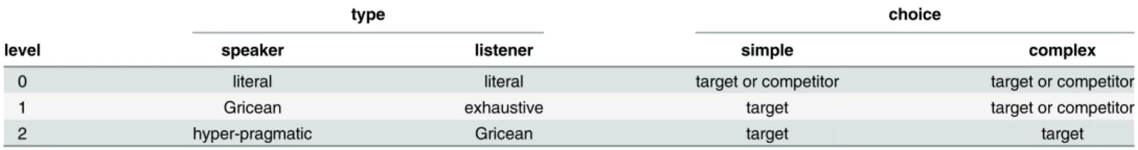
S1 Textfor a derivation of these predictions.)Table 1summarizes the reasoning types that we consider here, their level of Theory-of-Mind reasoning and the choices these idealized types would make in the simple and complex games fromFig 1.
Probabilistic reasoning types
Our goal is to infer, based on empirical data, which pragmatic reasoning types are plausible. In order to allow for slack, errors and mistakes when we fit a reasoning type model to potentially noisy empirical data, we formulate probabilistic variants of the idealized types fromTable 1. We then compare a homogeneous“null-model”that contains only the Gricean types to a“ satu-rated model”that contains all of the archetypes fromTable 1.
Homogeneous model
The homogeneous“null-model”is a version of the influential Rational Speech Act (RSA) model
[10]. TheRSAmodel defines parameterized probabilistic versions of a level-1 Gricean speaker
and a level-2 Gricean listener. Concretely, theRSAmodel implements a Gricean speaker with a
probabilistic tendency to prefer more informative true descriptions over less informative ones (where the strength of that tendency is a model parameter); and a Gricean listener who inter-prets expressions by forming a posterior belief, by Bayes’rule, on the assumption that the speaker behaves in the aforementioned fashion, while also factoring in the salience of objects in a given context (measured empirically; seeS4 Text).
The behavior of a hypothetical literal listenerR0is given by an unbiased choice of a referent
of which the received message is true. WithUthe uniform distribution overT:
R0ðtjmÞ ¼Uðtj t
0jm is true of t0
f gÞ:
RSA’s production rule is a probabilistic approximation to a rational choice of expression, given
the belief that the listener interprets literally (as defined byR0). More concretely, if the intended
referent ist, the speaker’s utility of sendingmis log(R0(tjm)), which measures the negative
(Kullback-Leibler) distance betweenR0’s belief after hearingmand the speaker’s degenerate probabilistic belief about the intended referent (i.e., the speaker knows who she wants to refer to). When the speaker has a degenerate beliefPS(tk) = 1 fortkthe intended referent, then if the
listener has beliefPL2Δ(T), utility in terms of negative Kullback-Leibler divergence reduces to:USðPS;PLÞ ¼ KLðPSjPLÞ ¼
P
iPSðtiÞlog
PSðtiÞ
PLðtiÞ¼ log
1
PLðtkÞ¼ logPLðtkÞ.
Table 1. Idealized pragmatic reasoning types and choices in the simple and complex reference games fromFig 1.
type choice
level speaker listener simple complex
0 literal literal target or competitor target or competitor
1 Gricean exhaustive target target or competitor
2 hyper-pragmatic Gricean target target
TheRSAmodel assumes that the speaker chooses messages with a probability that is
propor-tional to its expected success. This is implemented with a parameterized soft-max choice rule (e.g., [59–61]). The speaker’s expected choice probabilities are:
S1ðmjt;l; Þ /S
0
1ðmjt;lÞ þ; where
S0
1ðmjt;lÞ /expðl ðlogR0ðtjmÞÞÞ:
The parameterλ>0 measures, roughly put, the speaker’s rationality. Asλ! 1, the speaker would only make rational decisions, choosing the option that maximizes his expected utility. Asλ!0, the speaker chooses any true description with equal probability. The parameter allows a small positive probability for descriptions that are not true of the trigger referent. This, or something like it, is needed in an experimental approach like ours that allows the choice options of participants to deviate from semantic meaning.
Gricean listener behavior is given by Bayes’rule, based on the salience priorsS, which are empirically measured (seeS4 Text), and the behavior of a Gricean speakerS1:
R2ðtjm;l; Þ /SðtÞ S1ðmjt;l; Þ:
Heterogeneous model
Taken at face value, the above formulation of a single speaker and a single listener rule, in con-junction with the motivation that this is what a traditional Gricean approach would predict, seems to suggest thatallspeakers and listeners also individually conform to the predictions made byS1andR2. We want to explore the hypothesis that speaker and listener populations
are a mix of reasoning types that includes probabilistic variants of all the idealized reasoning types summarized inTable 1. In line with theRSAmodel we look at the following probabilistic
type rules (seeS2 Textfor motivation and formal details):
S0ðmjt;lÞ /expðlUðmj fm0 jm0 is true of tgÞÞ
R0ðtjm;lÞ /expðlUðtj ft
0 jmis true of t0gÞÞ
Snþ1ðmjt;l; Þ /S
0
nþ1ðmjt;lÞ þ
withS0
nþ1ðmjt;lÞ /expðllogRnðmjt;l! 1ÞÞ R1ðtjm;lÞ /expðlUR1ðt;mÞÞ
withUR1ðt;mÞ /UðtÞ S0ðmjt;
l! 1Þ
R2ðtjm;l; Þ /SðtÞ S1ðmjt;l; Þ
We will assume for modeling convenience that all reasoning types share aλand an(see also theGeneral discussionsection).
Nested modeling
The homogeneous model assumes that the population consists exclusively of Gricean types, while the heterogenous model is compatible with any population distribution over the three relevant speaker and listener typesS0,S1,S2,R0,R1andR2. Consequently, the homogeneous
model can be conceived of as a special case of the heterogeneous model, in the sense that the former fixes the population distribution to a single value (like a null-hypothesis would; in this case toS1andR2). Since the simpler model is a special case of the complex model, the latter will
simpler model. For example, some patterns of behavior in simple or complex reference games, as introduced previously, would seem incompatible with the simpler model, but unproblematic for the complex model (seeTable 1). One such pattern would be the observation of exclusively target choices in simple and complex conditions for production (suggesting that all subjects are individually level-2 reasoners), but an equal number of target and competitor choices for com-prehension (suggesting level-0 behavior). In order to test whether the more complex, heteroge-neous model is necessary or whether the null-model is sufficient, we therefore turn to
experimental data from tasks that require the comprehension and production of referential expressions, including drawing Quantity inferences of varying complexity.
Experiments
Experiment 1 tests the comprehension of referential expressions in reference games like the ones introduced inFig 1. Experiment 2 tests the production of referential expressions in the same games. Experiment 3 (seeS4 Text) elicits salience priors over objects required for model-ing theR2listener. Links to all experiments are provided inS3 Text.
Experiment 1: comprehension
Experiment 1 tested participants’behavior in a comprehension task that used instantiations of the“monsters and robots”reference games fromFig 1.
Participants. 60 participants were recruited via Amazon’s Web Service Mechanical Turk. Participants’IP address was limited to US addresses only. Only participants with a past work approval rate of at least 95% were accepted.
Ethics statement. This study was conducted with the approval of the Stanford University
research subjects review board. All participants gave written consent and received $1.00 for their participation (hourly rate of $10.00) according to the policies set forth by the Stanford University research subjects review board.
Procedure. Participants engaged in a referential comprehension task. On each trial they saw three objects on a display. Each object differed systematically along two dimensions: its ontological kind (robot, green monster, purple monster) and accessory (scarf, blue hat, red hat). In addition to these three objects, participants saw a pictorial message that they were told was sent to them by a previous participant whose goal was to get them to pick out one of these three objects. They were told that the previous participant was allowed to send a message expressing only one feature of a given object, and that the messages the participant could send were furthermore restricted to monsters and hats (i.e., there were no messages for referring to the robot or scarf feature; we refer to these features asinexpressible features). The four express-ible features were visexpress-ible to participants at the bottom of the display on every trial and are shown on the right side ofFig 1.
Participants initially completed four speaker trials. They saw three objects, one of which was highlighted with a yellow rectangle. Participants were asked to click on one of four pictorial messages to send to another Mechanical Turk worker to get them to pick out the highlighted object. They were told that the other worker did not know which object was highlighted but knew which messages could be sent. The four speaker trials contained three unambiguous and one ambiguous trial which could function as fillers in the main experiment.
Onsimple implicaturetrials, the target was generated by combining the feature denoted by the sampled message with the inexpressible feature along the other feature dimension. For example, if the sampled message was one of“red hat”or“blue hat”, the target was a robot with the respective hat. If instead the sampled message was“purple monster”or“green monster”, the target was the respective monster with a scarf. The competitor was generated by combining the feature denoted by the sampled message with a randomly sampled expressible feature along the other feature dimension. For example, if the sampled message was“red hat”, the competitor could be a green monster with a red hat or a purple monster with a red hat. The dis-tractor was generated by combining two features that were randomly sampled from the set of features that did not contain those features already present in target and competitor. For exam-ple, if the target was a robot with a red hat and the competitor was a green monster with a red hat, the distractor could be a purple monster with either a scarf or a blue hat.
Oncomplex implicaturetrials, the target was generated by combining the feature denoted by the sampled message with an expressible feature along the other feature dimension. For exam-ple, if the sampled message was“green monster”the target could be a green monster with a red hat. The competitor was generated by combining the feature denoted by the sampled message with the remaining expressible feature along the other feature dimension. Continuing our example, the competitor would then be a green monster with a blue hat. The distractor was generated by combining the target feature that was not denoted by the sampled message (red hat) with the inexpressible feature along the other feature dimension (robot).
Of the 42 filler trials, 24 used the displays from the implicature conditions but the target was a) the competitor from the simple condition (six trials), b) the distractor from the simple con-dition (six trials), or c) the competitor from the complex concon-dition (12 trials), as identified unambiguously by the trigger message. This was also intended to prevent learning associations of display type with the target. On the other 18 filler trials, the target was either entirely unam-biguous or entirely amunam-biguous given the message. That is, there was either only one object with the feature denoted by the trigger message, or there were two identical objects that were equally viable target candidates.Unambiguousandambiguousfillers were included as baselines to compare behavior on implicature trials to. Ambiguous fillers establish how often the target could be chosen by chance, while unambiguous fillers establish the upper bound on target choices. We did not include filler items where the target was the distractor from the complex condition, because this would have required participants to draw a one-step inference to iden-tify the target. Trial order as well as target, competitor, and distractor order were randomized.
Results and discussion. Those 15% of participants with the highest error rate (distractor responses) on trials that were not ambiguous were excluded from the analysis. This was done to avoid artificially inflating the noise parameter(see section on Bayesian model comparison below for further explanation). The 15% cutoff corresponded to a minimum error rate of 5% and included one participant who was not a self-reported native speaker of English. The data from the 51 remaining participants entered the analysis.
We were interested in participants’ability to draw simple and complex ad hoc Quantity implicatures. If participants always drew the implicature, their performance on critical trials should pattern with their performance on unambiguous filler trials. If instead they interpreted messages literally, their performance on critical trials should pattern with performance on ambiguous trials.
filler trials. On simple implicature trials, participants chose the target 77% of the time and the competitor 23% of the time. On complex implicature trials, the target was chosen less often (57% target choices vs. 42% competitor choices).
A logistic mixed-effects regression was conducted to assess whether the observed differences in target choices between the ambiguous and complex, and the complex and simple condition, were significantly different. Unambiguous trials were not included in the analysis because tar-get choices in this condition were at ceiling, i.e. there was not enough variance in participants’
responses to allow the model to converge. Trials on which the distractor was selected were excluded to allow for a binary outcome variable (target vs. competitor choice). This led to an exclusion of 1% of the data.
The model predicted the log odds of choosing a target over a competitor from a Helmert-coded CONDITION predictor. Two Helmert contrasts over the three relevant critical and filler conditions were included in the model, one comparing the simple implicature condition with the other two conditions (CONDITION(HARDER VS.SIMPLE)), and one comparing the complex
implicature to the ambiguous filler condition (CONDITION(AMBIGUOUS VS.COMPLEX). This allowed
us to capture whether the differences in choice distributions for neighboring conditions sug-gested byFig 2were significant.
We were also interested in whether participants displayed learning effects, i.e., whether they (maybe differentially) improved in the implicature conditions over the course of the experi-ment. To test this, the model also included a centered trial number predictor and the interac-tion of trial number and each of the Helmert contrasts. The model also included further control predictors for message type (accessory vs. species, centered) and target position (dummy-coded with left position as reference level). Finally, following [62], the model included the maximal random effect structure that allowed it to converge, which consisted in by-partici-pant intercepts as well as by-particiby-partici-pant slopes for message type and trial number.
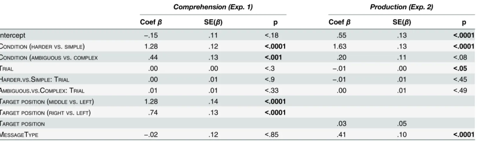
A model summary is shown inTable 2. As suggested byFig 2, participants made more target choices in simple than in complex implicature situations (β= 1.28,SE= .12,p<.0001), and they made more target choices in complex implicature situations than on ambiguous filler trials (β= .44,SE= .13,p<.001). This suggests that what we are calling simple implicatures are indeed simpler than what we are calling complex implicatures. Second, it suggests that, while participants performed similarly on complex and ambiguous trials, they nevertheless per-formed significantly above chance on complex trials. That is, at least some participants com-puted the more complex two-step implicatures at least sometimes. However, as shown in the Fig 2. Left: proportions of target, competitor, and distractor choices in Experiment 1. Error bars indicate 95% bootstrapped confidence intervals. Right: proportion of target choices in simple and complex conditions by participant. Dot size indicates number of participants.
right panel ofFig 2, the aggregate 77% (simple) and 57% (complex) target choice pattern was not mirrored on the individual participant level. That is, there was a lot of individual variability in participants’choice behavior. Some individuals succeeded more often on complex trials than others, and success on complex trials also made it more likely that that individual had a higher success rate on simple trials. This strongly suggests that participants in this experiment were a mixture ofR1exhaustifiers andR2Gricean listeners.
Neither the main effect of trial number nor its interactions with the two Helmert contrasts reached significance, suggesting that there were no learning effects in this study, i.e. partici-pants’behavior on both implicature and filler trials remained constant throughout. This is important for our subsequent model comparison, which assumes that participants are of a fixed reasoning type.
Finally, both target position effects reached significance: participants were more likely to choose the target if it was in the center (β= 1.28,SE= .14,p<.0001) or right (β= .71,SE= .13, p<.0001) compared to the left position in the display. There was no multicollinearity between fixed effects to speak of (all variance inflation factors<1.33).
This experiment constitutes a replication of Experiment 1 of [9]. The data from all four con-ditions will be used in model comparison on the homogeneous and heterogeneous model. Of interest is whether the individual participant variability suggested byFig 2is substantial enough to warrant the additional complexity introduced by allowing for heterogeneous types. But first we report the results of the complementary production study.
Experiment 2: production
Experiment 2 tested participants’behavior in a production task within the same reference game setting as Experiment 1.
Participants. 60 participants were recruited via Amazon’s Web Service Mechanical Turk. Participants’IP address was limited to US addresses only. Only participants with a past work approval rate of at least 95% were accepted.
Ethics statement. This study was conducted with the approval of the Stanford University
research subjects review board. All participants gave written consent and received $1.00 for their participation (hourly rate of $10.00) according to the policies set forth by the Stanford University research subjects review board.
Table 2. Summary of coefficients, standard errors, andp-values for the comprehension (Experiment 1, left) and production (Experiment 2, right) models.Significantp-values are shown in boldface. Predictors coding experimental conditions of interest, predictors coding learning effects, and other con-trol predictors are separated from each other by horizontal lines.
Comprehension (Exp. 1) Production (Exp. 2)
Coefβ SE(β) p Coefβ SE(β) p
Intercept −.15 .11 <.18 .55 .13 <.0001
CONDITION(HARDER VS.SIMPLE) 1.28 .12 <.0001 1.63 .13 <.0001
CONDITION(AMBIGUOUS VS.COMPLEX .44 .13 <.001 .20 .11 <.08
TRIAL .00 .00 <.3 −.01 .00 <.05
HARDER.VS.SIMPLE: TRIAL .00 .01 <.9 −.01 .01 <.45
AMBIGUOUS.VS.COMPLEX: TRIAL .01 .01 <.33 .00 .01 <.49
TARGET POSITION(MIDDLE VS.LEFT) 1.28 .14 <.0001
TARGET POSITION(RIGHT VS.LEFT) .74 .13 <.0001
TARGET POSITION .03 .05
MESSAGETYPE −.02 .12 <.85 .41 .10 <.0001
Procedure and Materials. The procedure was identical to that on speaker trials in Experi-ment 1.
Each participant saw 66 experimental trials. The distribution of trial types was the same as in Experiment 1: 24 critical trials (12 simple, 12 complex, seeFig 1) and 42 filler trials. Each of the four messages received a trial by trial status as target, competitor, distractor 1, or distractor 2. Stimuli were created by randomly sampling a message and then generating a grid of three objects following different constraints in different conditions. The sampled message was the target.
Onsimple implicaturetrials, the trigger object was generated by combining the feature denoted by the sampled message with an expressible feature along the other feature dimension. The message denoting this other feature was the competitor message. For example, if the sam-pled message was“green monster”, the trigger object might be a green monster with a red hat. The target message was then“green monster”, the competitor message“red hat”. A second object was generated by combining the feature denoted by the competitor message with the inexpressible feature along the other feature dimension. In our example, the second object would be a robot with a red hat. A third object was generated by combining the two remaining expressible features. The messages denoting these features were randomly deemeddistractor 1 ordistractor 2.
Oncomplex implicaturetrials, the trigger object was generated by combining the feature denoted by the sampled message with an expressible feature along the other feature dimension. The message denoting this other feature was the competitor message. For example, if the sam-pled message was“green monster”, the trigger object might be a green monster with a red hat. The target message was then“green monster”, the competitor message“red hat”. A second object was generated by combining the feature denoted by the competitor message with the inexpressible feature along the other feature dimension. In our example, the second object would be a robot with a red hat. A third object was generated by combining the feature denoted by the sampled message with the remaining expressible feature along the other feature dimen-sion. In our example: a green monster with a blue hat. The remaining messages were randomly deemeddistractor 1ordistractor 2.
Of the 42 filler trials, 24 used the displays from the implicature conditions but the highlighted trigger object was a) the competitor from the simple condition (six trials), b) the distractor from the simple condition (six trials), or c) the distractor from the complex condi-tion (12 trials). We did not include filler items where the trigger was the competitor from the complex condition, because this would have required participants to draw a one-step inference to select the target message. On the remaining 18 filler trials, the target message to refer to the highlighted object was either entirely unambiguous (because the other feature was one of the inexpressible robot or scarf features) or entirely ambiguous (because no other object in the dis-play had the trigger object features but each trigger object feature was an equally good message choice).Unambiguousandambiguousfillers were included as baselines to compare behavior on implicature trials to. On unambiguous trials, the trigger object had one expressible and one inexpressible feature, such that the target message denoted the expressible feature. No other objects in the display shared that feature. On ambiguous trials, the trigger object had two expressible features that no other object in the display shared. Ambiguous fillers establish how often the target message would be chosen by chance, while unambiguous fillers establish the upper bound on target message choices. Trial order, position of the trigger object in the grid, and order of target, competitor, and distractor messages were randomized.
task. For example, participants were asked to choose between four, rather than three, alterna-tives. The exclusion included two participants who were not self-reported native speakers of English. The data from the 50 remaining participants entered the analysis.
Proportions of choice types are displayed inFig 3on the left. We collapse the two distractor types into one distractor category, since the difference is of no theoretical interest and there were no differences in the choice distributions between the two categories. As expected, partici-pants were close to ceiling in choosing the target on unambiguous filler trials (96% target choices vs. 1% competitor choices) but at chance on ambiguous ones (48% target choices vs. 48% competitor choices). On critical implicature trials, participants’performance was interme-diate between ambiguous and unambiguous filler trials. On simple implicature trials, partici-pants chose the target 82% of the time and the competitor 16% of the time. On complex implicature trials, the target was chosen less often (53% target choices vs. 45% competitor choices).
The mixed effects logistic regression analysis was conducted as in Experiment 1 and pre-dicted target over competitor message choices. The only differences were that a) the random effects structure consisted only of random by-participant intercepts (because more complex random effects structures did not allow the model to converge) and b) target position was coded as a centered numeric position (1 to 4).
A model summary is shown inTable 2. As suggested byFig 3, participants made more target choices in simple than in complex implicature situations (β= 1.63,SE= .13,p<.0001). In con-trast to the comprehension study, participants only made marginally more target choices in complex implicature situations than on ambiguous filler trials (β= .2,SE= .11,p<.08), suggest-ing that complex inferences are more difficult to draw in production than in comprehension.
In addition to the theoretical effects of interest, there was a main effect of trial number, such that participants became overall slightly less likely to choose targets as the experiment pro-gressed (β= -.01,SE= .003,p<.05). However, this effect was so small compared to the other significant fixed effects that it is not of interest. Neither interaction of trial number with the two Helmert contrasts reached significance, suggesting that participants’behavior did not change differentially for the different conditions.
Finally, of the additional control predictors only that of message type reached significance: participants were more likely to choose the target message if the message denoted a species Fig 3. Left: proportions of target, competitor, and distractor choices in Experiment 2. Error bars indicate 95% bootstrapped confidence intervals. Right: proportion of target choices in simple and complex conditions by participant. Dot size indicates number of participants.
rather than an accessory. There was no multicollinearity between fixed effects to speak of (all variance inflation factors<1.16).
This experiment constitutes a replication of Experiment 2 of [9], with some caveats: the rank order of target choice proportions is as in [9]. However, here we find that target choices are slightly above chance in the complex condition and target choices are not at ceiling in the simple condition. These differences may be due to the size of the sample used in this experi-ment, which was larger and thus made it possible to detect smaller effects. The data from all four conditions will be used in the model comparison of the homogeneous and heterogeneous model. As was the case for the comprehension data reported previously, the individual target choice distributions shown inFig 3on the right suggest that in production, too, rather than mirroring the aggregate 82% (simple) and 53% (complex) target choice proportions, individual participants displayed systematic differences in response behavior.
Model fits and model comparison
The main goal of this section is to assess whether it is plausible to maintain the“null hypothe-sis”that all participants in our experiments can be construed as Gricean, i.e., asS1andR2
respectively. The“alternative hypothesis”is that our data are better captured by assuming that the population of participants is a heterogeneous mix of various reasoning types.
Our conclusion will be that, despite the added complexity of the heterogeneous model, the level comprehension data strongly favor the more complex model. The individual-level production data, on the other hand, suggest that most (though not all) speakers were Gri-cean in our experiment. For production, there is a large majority of likely GriGri-ceanS1speakers,
but for comprehension there is no majority of GriceanR2listeners. What the remainder of this
section adds to this is a careful model comparison that weighs predictive accuracy against model complexity. Such model comparison is needed because mere inspection of the choice data alone or inspection of posteriors over reasoning types (see below), will not allow precise assessments: e.g., is it enough evidence to favor the complex model over the simpler model that four participants from our pool are most likely literal speakers?; could the simpler model still be plausibly maintained, given its elegant parsimony, despite the fact that only a minority of subjects are most likely Gricean listeners of level-2? Normatively compelling answers to these questions hinge on the relative complexity of models and on the relative success of explaining the observed data. The Bayesian model comparison of this section offers exactly that.
Gricean types match the population-level data
Before looking at individual-level data, it is worth noting that, like in previous studies on refer-ence games, the Gricean types alone seem to capture the population-level data reasonably well. Abstracting away from salience priors and stochasticity in the choice rules, Gricean speakersS1
should be able to solve the simple, but not the complex condition, while Gricean listenersR2
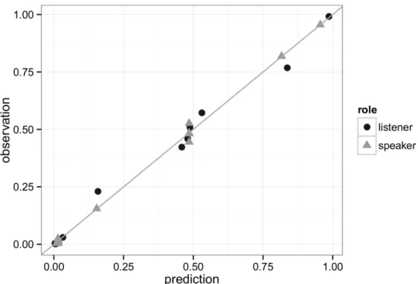
should be able to solve both. The population-level average data, plotted in Figs2and3on the left, show this only in tendency. But if we add salience and noise, the observed choice frequen-cies can be approximated rather well by the homogeneous model. Previous studies have looked at point-estimates for parameters like ourλand, obtained by minimizing the squared distance between the observed choice frequencies and the predicted choice probabilities [7]. Best fitting parameters in this sense areλ= 2.533 and= 0.015 (production) andλ= 1.597 and= 0.005 (comprehension). Resulting predictions are well-aligned with the observations, as shown inFig 4(correlationr= 0.997,p<0.0001). By this standard, the GriceanRSAmodel appears to be a
A hierarchical model for individual-level data
That a population average is well approximated by some mathematical function does not imply that the individual-level data must conform to it as well [22–24]. It is therefore relevant to look at each individual’s choice data as the to-be-explained observations. A first goal is to infer, based on each individual’s choice data, an estimate of each individual’s likely reasoning type. A second goal is to determine whether the simpler Gricean model is sufficient for explain-ing the data, or whether the added complexity of the heterogeneous model is necessary. To achieve both goals, we take a hierarchical modeling approach [63] in which the simpler Gricean model is nested under the more complex heterogeneous type model.
The general idea behind this approach is that we specify for each participantia latent type τi2{0, 1, 2} that captures the depth of pragmatic reasoning ofi. Eachτiis drawn from atype
distribution Pτthat captures the probability of sampling reasoning types from the population from which our participants were sampled. Our data will then provide information about the likelihood that each participant is a pragmatic reasoner of level 0, 1, or 2andabout the general population distribution of reasoning types. The homogeneous model is a special case of the heterogeneous model in that it assumesa priorionly one value for the type distributionPτ.
More concretely, the data that we would like to explain are countsdX
ijk, one set for produc-tion (X=S) and one for comprehension (X=R), giving the number of choices across the whole experiment of participantifor gamej(simple, complex, unambiguous, ambiguous) that fell into categoryk(target, competitor, distractor 1, possibly also distractor 2 for production). Every participant saw each gamejafixed number of timesnX
j. We assume that each participant ihas afixed typeτi2{0, 1, 2} that is constant across the experiment. The assumption of Fig 4. Probabilistic predictions of theRSAmodel under best-fitting parameter values (see main text), plotted
against the observed choice frequencies.Each dot represents one choice option in one of our four reference games.
temporally consistent reasoning types is generally dubious, but necessary to keep the model manageable. However, in our case this assumption seems warranted given the lack of relevantly significant trial effects in our regression analyses reported above.
For production, a participant’s type fixes whether that participant is a literalS0, a GriceanS1
or a hyper-pragmaticS2speaker. For comprehension, a participant’s type fixes whether that
participant is a literal listenerR0, an exhaustifierR1or a Gricean listenerR2. The likelihood of
eachdX
ijkis then given by the binomial distribution, with a probabilityP X
ijkthat depends on the participant’s typetX
i, error rate
X, rationalityλX, and gamej:
dX
ijkBinomialðP X ijk;n
X jÞ P
X
ijk¼Xtiðkjgamej;;lÞ;
where the latter is defined by the probabilistic choice types of the heterogeneous model that were introduced previously.
We assume largely uninformative prior probabilities for parameter values (the structure is the same for production and comprehension, so we omit the variableXfor readability):
Gammaðshape¼:25;rate¼:1Þ lGammaðshape¼2;rate¼:5Þ
t
iCategoricalðP
t
Þ Pt
Dirichletð1;1;1Þ
The use of these gamma distributions is motivated by the idea that we expect tremblesto be very small, possibly even 0, but thatλwould be positive, but rather small as well.
The full probabilistic model is sketched also inFig 5, using the conventions of [64]. Rea-soning typesτiare sampled from a categorical distribution with a population-leveltype distri-bution Pτ. In other words, the model assumes that there is a distribution of reasoning types from which our sample of participants was drawn.A priorithe heterogeneous modelMhet considers any type distributionPτequally likely, so that we sample it from a Dirichlet distri-bution with uniform weight 1 for all dimensions. That means thatMhomis nested underMhet as the special case wherePτ=h0, 1, 0ifor the speaker population andPτ=h0, 0, 1ifor the lis-tener population.
Posteriors over model parameters
To learn abouta posterioricredible values of parameters we used JAGS [65] to collect 10000 samples from the joint posterior distribution after a burn in of 10000 samples, from two chains with a thinning factor of 2. This set-up ensured convergence to the stationary distribution, with theR^value of all continuous variables below 1.1 [66].
Summary statistics for the estimated marginal posteriors of model parameters are given in
Table 3. Estimated marginal densities for the population priors are shown inFig 6. The produc-tion data suggest that most speakers areS1Gricean maximizers of relevant information, but
also attest a small proportion of literalS0speakers. In contrast, the data appear to give little
sup-port to hyper-pragmaticS2speakers. These results are roughly in line with the homogeneous
model, which assumes that speakers are of typeS1. In contrast, the comprehension data give
non-negligible levels of posterior credence to all three listener types. Interestingly, the Gricean listenersR2are less likely than exhaustive listenersR1, and possibly even less likely than literal
listenersR0. This seems to contradict the idea ofR2-homogeneity in the population quite
clearly, but proper model comparison is required to factor in model complexity as well (see below).
that is most likely a hyper-pragmaticS2speaker and there are four participants identified as
most likely being literalS0speakers. For most participants in the production experiment, our
posterior beliefs in what type they should be, given the model and the data, have little uncer-tainty. In contrast, the comprehension data also identified most participants as almost certainly being of a single reasoning type, but there is somewhat more uncertainty in some cases. Never-theless, there are only three participants whose classification by model and data yields ambigu-ous results. Interestingly, for all reasoning types, there are several participants that are clearly identified as most likely belonging to that type.
Table 3. 95% highest density intervals and means of marginal posteriors.
speaker listener
HDI min mean HDI max HDI min mean HDI max
9.5e-3 0.012 0.01498 1.88e-16 2.43e-4 1.11e-3
λ 2.956 3.330 3.711 5.424 5.856 6.298
τ0 0.036 0.117 0.209 0.173 0.301 0.442
τ1 0.741 0.843 0.940 0.410 0.560 0.703
τ2 8.43e-05 0.040 0.095 0.054 0.139 0.236
doi:10.1371/journal.pone.0154854.t003
Fig 5. Sketch of the full data-generating model as a probabilistic graphical model, using the
conventions of [64].The more abstract a parameter, the higher it is in the graph. Deterministic variables have double edges. Categorical variables have rectangular shape. Observed variables are shaded in gray. Boxes encircle the range of indices.
Bayesian model comparison
When comparing models of different complexity, we need to weigh predictive accuracy against model parsimony. A Bayesian approach to model comparison does that [35,36,67–69]. Given our dataD, we are interested in the ratioP(MhomjD)/P(MhetjD) of posterior plausibility in favor of the simpler homogeneous modelMhomover the more complex heterogeneous modelMhet given our dataD. By Bayes’rule this is the product of the ratio of the models’evidencesand the ratio of their prior probability:
PðMhomjDÞ PðMhetjDÞ ¼
PðDjMhomÞ PðDjMhetÞ
PðMhomÞ PðMhetÞ : Fig 6. Marginal posterior for type priorsPτ
(τi).
doi:10.1371/journal.pone.0154854.g006
Fig 7. Marginal posterior for participants' reasoning typesτi.
Irrespective of the strength of our prior beliefs in the models, the relative change in our belief brought about by the data is theBayes factor P(DjMhom)/P(DjMhet), which integrates over the predictions of the models under all its free parameter values, and thereby implements a bias against overfitting and model complexity:
PðDjMhomÞ PðDjMhetÞ
¼
R
PðyjM
homÞPðDjy;MhomÞ dy
R
PðyjM
hetÞPðDjy;MhetÞ dy :
Here,θis a vector of values for all free model parameters.P(θjMhom) andP(θjMhom) are the
priors over these under the respective models. The vectorθis the same for both models, but, as shown above, under the hierarchical approach taken here, the homogeneous model isnested under the heterogeneous model as the special case whereP(Pτ=h0, 1, 0i jMhom) = 1 for the speaker population andP(Pτ=h0, 0, 1i jMhom) = 1 for the listener population.
Although the computation of Bayes factors can be difficult in general, there is an alternative, easier method for calculating Bayes factors of nested models, theSavage-Dickey density-ratio [34,70]. Unfortunately, even with this method, precise calculation of Bayes factors is beyond reach for the complex models at hand. But approximation by simulation is possible. (Details and further explanations are provided inS5 Text.) To avoid precision problems, we look at the less extreme“null-hypotheses”:Pt
¼ he
2;1 e;
e
2ifor production andP t
¼ he
2;
e
2;1 eifor
comprehension. The higher we choosee, the more charitable we are to the homogeneous model (which is then no longer properly homogeneous, but still“approximately homoge-neous”). With the fairly charitable value of 0.05, we receive Bayes factor approximations of:
PðDprodjMhomÞ PðDprod jMhetÞ
3:955 PðDcomp jMhomÞ
PðDcompjMhetÞ
2:8e 11:
Bayes factors greater than 1 suggest that the data provide evidence in favor of the simpler homogeneous model. A standard recommendation is that only Bayes factors greater than 3 count as sufficiently strong evidence in favor of a model [34]. This means that under the chari-table alternative“null-model”that says that exactly 95% of participants are GriceanS1speakers,
our data favor the simpler“almost only Gricean”model: its predictive success may be inferior, but due to factoring in model complexity, the posterior odds are shifted slightly towards it. However, if we lower our tolerance and test the assumption that exactly 99% of all participants are GriceanS1speakers (e= 0.01), we obtain a Bayes factor of only 0.004 in favor of the Gricean
model, i.e., very strong support for the more complex heterogeneous model (1/0.004250). In sum, the data support a moderate version of the idea that a large majority of speakers are Gri-cean, and even favors such a model over the full complexity and underspecification of the het-erogeneous model, but our data do not support the idea that that majority is arbitrarily close to 100%.
On the other hand, even if we assume 95% GriceanR2listeners, the odds are very clearly in
favor of the complex heterogeneous model. This is also evident from the inferred most likely types of individual participants, shown inFig 7: very few participants’choice behavior can be best explained by the homogeneous model’s comprehension rule. What the Bayes factor analy-sis adds is the certainty that the heterogeneous model’s complexity isnecessaryfor a decent explanation of the comprehension data; in other words, assuming that almost everybody is a Gricean listener is not a good explanation of the individual-level data.
Taken together, we reach the nuanced conclusion that the homogeneous Gricean model is half-supported by our data. Under a charitable interpretation, the idea that most (though not all) speakers are GriceanS1speakers can be maintained, but not the idea that most listeners are
listeners. That is, there is variation in participants’linguistic choices: a majority of participants use simple informativity-based heuristics, but a non-negligible number engages in deeper ToM-reasoning.
General discussion
Recent years have seen a surge of success for probabilistic approaches to pragmatics, which have translated the Gricean picture of language use into a formal framework that makes quan-titative, empirically testable predictions for speaker and listener behavior [7,10,12–14,16–18,
20,21]. In line with Grice’s original considerations, many of these approaches treat language users as Gricean speakers (S1) and Gricean listeners (R2). The models developed in this
frame-work have provided a very good fit to aggregate population-level data across many different pragmatic tasks, suggesting that speakers and listeners are, on average, rational Gricean agents.
In contrast, individual-level data from our experiments on reference games suggest that it makes sense to believe that the population of participants is heterogeneous. While Gricean speakers and Gricean listeners are attested, the majority of participants seems to apply an infor-mation-based heuristic, corresponding to level-1 Theory-of-Mind reasoning: the majority of speakers are Gricean (S1), but the majority of listeners are exhaustive listeners (R1). This is
despite the fact that a homogeneous Gricean population model does explain the population-level average reasonably well.
Although these results are contingent on the particular task we presented participants with, the obtained data, and the specific modeling choices we made, the demonstration that there can be discrepancies between the population- and individual-level perspective has at least two important implications for the growing field of probabilistic pragmatics, one more technical and one more conceptual. First, for probabilistic pragmatics to ripen, it is important in general to compare different relevant model variants stringently based on empirical data, especially when these variants are attested in the extant theoretical literature. Secondly, that individual differences in cognitive performance exist in many domains is beyond doubt, but the question arises whether a computational-level probabilistic pragmatics can accommodate these and whether it should care to do so. We will expand on these points in the following.
Model variants & model comparison
Bayesian approaches to cognition have repeatedly been criticized as appearing conceptually under-motivated and as having insufficiently explored plausible alternatives [71–73]. Our con-tribution here is a partial response to these points of criticism, for we have pitted different vari-ants of probabilistic pragmatic models against each other. In general, we believe that explicit model comparison is necessary in order to refine models and better understand what probabi-listic pragmatics can and cannot achieve. Comparison of variants is especially relevant in cases like ours where the extant theoretical literature offers clearcut and plausible alternative model-ing choices. When several model variants are conceivable, it can also be the case that these vari-ants co-exist. In that case, hierarchical mixture models suggest themselves. We have tried to show here, by way of an example, how such hierarchical modeling could enrich the perspective of probabilistic pragmatics.
could capture the behavior of all other types as well, simply by choice of appropriateλs ands. In this sense, individual variation in terms of reasoning types is not subsumed by individual variation in error levels. Moreover, although level-0 types can be emulated by level-(n 1)-types withλclose to 0, this is uninteresting as long as the research question is not whether a particular mathematical model can account for the data, but whether a particular conceptual idea can (e.g., literal interpretation vs. Gricean interpretation).
Individual differences in probabilistic pragmatics
Probabilistic pragmatic models of the kind considered here are usually taken to provide computational-level analyses of pragmatic phenomena rather than algorithmic-level ones [74]. That is, the modeler specifies the problem that the agent needs to solve and provides a rational solution strategy, while making minimal assumptions about resource limitations [75]. Why should such a computational-level rational analysis care about individual differences?
First, if only aggregate data are considered, it is possible that the phenomenon we are trying to explain is an artifact of averaging [76]. If half the population is risk seeking and half is risk averse (to the same extent), then the average would indicate: the group is risk neutral. What would it then mean to explain risk neutrality as an optimal adaptation to functional pressure from the environment? In such an extreme case, a model that purportedly shows how the observed average behavior is rational need not be a model of anybody actually behaving ratio-nally. This would be an odd instance of rational analysis: we would explain how adaptive pres-sure of the environment selected the group’s average behavior, not each individual’s behavior. Maybe such a line of explanation is possible, but in order to avoid these philosophical difficul-ties, inspection of individual-level data is key. If individual-level behavior aligns nicely with the average (modulo well-behaved noise) nothing is amiss.
If it does not, there are additional advantages to incorporating individual differences into computational-level models. One is bringing probabilistic pragmatics models closer to other processing-oriented models in psycholinguistics. Allowing for individual differences is one way of incorporating assumptions about varying degrees of resource limitations while remaining agnostic about what the algorithmic-level processes are that give rise to different computa-tional-level player types. Nevertheless, one can speculate: plausible candidates are limitations on working memory, executive control, and other cognitive resources. In fact, there is a large body of literature identifying a role for these kinds of factors in language processing, theory of mind, and reasoning, which arguably constitute the intersection at which pragmatics lies. For example, speakers’word order preferences are affected by working memory [77], differences in gesture production have been shown to be associated with individual differences in working memory as well as in spatial and verbal abilities [78,79], working memory affects the rate at which prosody triggers contrastive inferences [80], and differences in perspective-taking have been shown to correlate with differences in inhibitory control [81]. In the reasoning literature, there is a large body of work showing that different cognitive biases (like the anchoring effect, belief bias, overconfidence bias, hindsight bias, base rate neglect, outcome bias, and sunk cost effect) are associated with differences in different types of intelligence, cognitive reflection, and openness (e.g., [82]). In this way, acknowledging individual differences and applying rational analysis at the individual level may help integrate computational-level probabilistic models with processing-oriented approaches.
null effects when different subpopulations apply different parsing strategies [83]. Moreover, if the goal is to improve the predictive power of our cognitive models, what we have shown here is that taking into account individual differences is necessary for some cases of pragmatic rea-soning. Whether it is necessary for all cases is an empirical question that should be addressed in future work. Relatedly, whether an individual’s inferred player type on one pragmatic task transfers to another pragmatic task is another interesting open question.
For all the above discussed reasons, an empirically adequate theory of pragmatic language use might ultimately like to predict individuals’behavior, not just population-level means. A final illustration of this point comes from taking the perspective of a speaker engaged in dialog. Speakers tend to not speak into a vacuum, but instead interact with a particular interlocutor about whose behavior they may have rather concrete beliefs. When speaking with a complete stranger, speakers may start out with the assumption that their interlocutor is like the popula-tion mean. However, speakers and listeners immediately obtain informapopula-tion about their inter-locutor’s identity that they condition on. Indeed, there is an increasing body of work showing that interlocutors rapidly adapt to each others’phonetic [84], lexical [85], and syntactic prefer-ences [86,87]. One of the interlocutor’s attributes is arguably the amount of effort they can or are willing to invest in drawing inferences, or, put differently: their player type. If I know my interlocutor’s type, I can make more accurate predictions about their use of language, thereby increasing the chance of communicative success. This entails that interlocutors should track each others’player type. Some evidence that they do comes from studies on speaker-specific overinformativeness, showing that listeners rapidly adapt to the level of informativeness of speakers’use of adjectives [25,26], but much more work is needed to investigate the extent to which interlocutors represent player type.
Conclusion
In this paper we set out to answer a simple question: are listeners and speakers Gricean at the individual level or only at the population level? To test this, we inferred individually variable pragmatic reasoning types as latent parameters in a hierarchical model and used Bayesian model comparison to draw conclusions about whether the added complexity of maintaining the possibility of non-Gricean reasoning types is required by our data. Data came from one production and one comprehension study in reference games that required participants to apply pragmatic reasoning of varying complexity. While there was evidence for a substantial number of likely Gricean speakers and Gricean listeners, the added complexity of considering additional reasoning types was justified, especially in comprehension, where many listeners were identified as exhaustifiers. In conclusion, given our data for this task and our model, there are clear individual differences between participants; for the case of Quantity inferences in ref-erential expressions, most speakers and listeners seem to apply an information-based heuristic, corresponding to level-1 ToM-reasoning. This suggests that probabilistic pragmatics models should take into account potential individual variation, even if designed as a computational-level theory, and this paper demonstrates one way of doing so.
Supporting Information
S1 Text. Derivation of Predictions for Idealized Reasoning Types.
(PDF)
S2 Text. Explanation of Heterogeneous Type Definitions.
S3 Text. URLs for Experiments.
(PDF)
S4 Text. Details on the Prior Elicitation Experiment.
(PDF)
S5 Text. Details on the Calculation of Bayes Factors.
(PDF)
S6 Text. Posterior Predictive Check for Heterogeneous Model.
(PDF)
S1 Data. Data from Experiment 1.
(CSV)
S2 Data. Data from Experiment 2.
(CSV)
Acknowledgments
We would like to thank Noah D. Goodman and Gerhard Jäger for valuable discussion.
Author Contributions
Conceived and designed the experiments: JD MF. Performed the experiments: JD. Analyzed the data: JD MF. Wrote the paper: JD MF.
References
1. Matsumoto Y. The Conversational Condition on Horn Scales. Linguistics and Philosophy. 1995; 19(1):21–
60. doi:10.1007/BF00984960
2. Horn LR. Fromiftoiff: Conditional Perfection as Pragmatic Strengthening. Journal of Pragmatics. 2000; 32:289–326. doi:10.1016/S0378-2166(99)00053-3
3. Grice PH. Logic and Conversation. In: Cole P, Morgan JL, editors. Syntax and Semantics, Vol. 3, Speech Acts. New York: Academic Press; 1975. p. 41–58.
4. Franke M, Jäger G. Probabilistic pragmatics, or why Bayes’rule is probably important for pragmatics. Zeitschrift für Sprachwissenschaft. 2016; 35(1):3–44.
5. Bott L, Noveck IA. Some Utterances are Underinformative: The Onset and Time Course of Scalar Infer-ences. Journal of Memory and Language. 2004; 51(3):437–457. doi:10.1016/j.jml.2004.05.006 6. Breheny R, Katsos N, Williams J. Are Generalised Scalar Implicatures Generated by Default? An
On-Line Investigation into the Role of Context in Generating Pragmatic Inferences. Cognition. 2006; 100 (3):434–463. doi:10.1016/j.cognition.2005.07.003PMID:16115617
7. Goodman ND, Stuhlmüller A. Knowledge and Implicature: Modeling Lanuage Understanding as Social Cognition. Topics in Cognitive Science. 2013; 5:173–184. doi:10.1111/tops.12007PMID:23335578 8. Degen J, Tanenhaus MK. Processing scalar implicature: A Constraint-Based approach. Cognitive
Sci-ence. 2015; 39(4):667–710. doi:10.1111/cogs.12171PMID:25265993
9. Degen J, Franke M. Optimal Reasoning About Referential Expressions. In: Brown-Schmidt S, Ginzburg J, Larsson S, editors. Proceedings of SemDial 2012 (SeineDial): The 16thWorkshop on the Semantics
and Pragmatics of Dialogue; 2012. p. 2–11.
10. Frank MC, Goodman ND. Predicting Pragmatic Reasoning in Language Games. Science. 2012; 336 (6084):998. doi:10.1126/science.1218633PMID:22628647
11. Rohde H, Seyfarth S, Clark B, Jäger G, Kaufmann S. Communicating with Cost-Based Implicature: A Game-Theoretic Approach to Ambiguity. In: Brown-Schmidt S, Ginzburg J, Larsson S, editors. Pro-ceedings of SemDial 2012 (SeineDial): The 16thWorkshop on the Semantics and Pragmatics of
Dia-logue; 2012. p. 107–116.