Markov approach to evaluate the availability simulation model for power generation system in a thermal power plant ,

(1)

* Corresponding author.

Contents lists available at GrowingScience

International Journal of Industrial Engineering Computations

homepage: www.GrowingScience.com/ijiec

Markov approach to evaluate the availability simulation model for power generation system in a thermal power plant

Ravinder Kumara*, Avdhesh Kr. Sharmaaand P.C Tewarib

a

Department of Mechanical Engineering, D.C.R University of Science & Technology Sonepat, India

b_{Department of Mechanical Engineering, National Institute of Technology Kurukshetra, India}

A R T I C L E I N F O A B S T R A C T

Article history: Received 22 April 2012 Received in revised format 7 July 2012

Accepted July 19 2012 Available online 15 August 2012

In recent years, the availability of power plants has become increasingly important issue in most developed and developing countries. This paper aims to propose a methodology based on Markov approach to evaluate the availability simulation model for power generation system (Turbine) in a thermal power plant under realistic working environment. The effects of occurrence of failure/course of actions and availability of repair facilities on system performance have been investigated. Higher availability of the components/equipments is inherently associated with their higher reliability and maintainability. The power generation system consists of five subsystems with four possible states: full working, reduced capacity, reduced efficiency and failed state. So, its availability should be carefully evaluated in order to foresee the performance of the power plant. The availability simulation model (Av.) has been developed with the help of mathematical formulation based on Markov Birth-Death process using probabilistic approach. For this purpose, first differential equations have been generated. These equations are then solved using normalizing condition so as to determine the steady state availability of power generation system. In fact, availability analysis is very much effective in finding critical subsystems and deciding their preventive maintenance program for improving availability of the power plant as well as the power supply. From the graphs illustrated, the optimum values of failure/repair rates for maximum availability, of each subsystem is analyzed and then maintenance priorities are decided for all subsystems.The present paper highlights that in this system, Turbine governing subsystem is most sensitive demands more improvement in maintainability as compared to the other subsystems. While Turbine lubrication subsystem is least sensitive.

Keywords:

Availability simulation model Transition diagram Probabilistic approach Markov approach Stochastic analysis

1. Introduction

(2)

the issues that are gaining importance in industry. The production suffers due to failure of any intermediate system even for small interval of time. The cause of failure may be due to poor design, system complexity, poor maintenance, lack of communication and coordination, defective planning, lack of expertise/experience and scarcity of inventories. Thus, to run a process plant highly skilled/ experienced maintenance personnel are required. Woo (1980) performed a study on reliability of an experimental fluidized-bed boiler of a coal-fueled plant to determine the major contributors to plant outage in terms of equipment failure and plant management. Most power plants use the index proposed by IEEE Std. 762, (1987), to define availability. During the past decade a lot of study has been done by Butler (1986), Koren (1987) and Ciardo et al. (1989) on analysis tools for reliability, availability, performance and performability modeling. Kumar et al. (1988) discussed about feeding systems in the sugar industry and paper industry. Kumar and Singh (1989) analyzed the Availability of a washing system in paper industry. The considerable efforts have been made by the researchers providing general methods for prediction of system reliability designing equipments with specified reliability figures, demonstration of reliability values issues of maintenance, inspection, repair and replacement and notion of maintainability as design parameter, as stated by Sharma (1994). Kaushik and Singh (1994) presented reliability analysis of the feed water system in a thermal power plant. Rahman et al. (2010) worked on root cause failure analysis of a division wall superheater tube of a coal-fired power station in Kapar Power Station, Malaysia. Purbolaksono et al. (2010) had undergone failure case studies of SA213-T22 steel tubes of the reheater and superheater of boiler using computer simulations. Lim and Chang (2000) studied a repairable system modeled by a Markov chain with two repair modes. Samrout et al. (2005) describes the availability and reliability as good evaluations of a system’s performance. Barabady and Kumar (2007) states that the most important performance measures for repairable system designers and operators are system reliability and availability. Kiureghian and Ditlevson (2007) analyzed the availability, reliability and downtime of system with repairable components. Jorn Vatn and Aven (2010) discussed the optimization of maintenance interval using classical cost benefit analysis approach in Norwegian railways. So it is imperative to investigate the availability analysis of the unit, for taking necessary measures regarding maximization of power supply. This paper presents a system reliability-based method to identify the most critical subsystem in the system discussed. The criticality of a subsystem as for power generation operation is associated with the subsystem failure effect on the system operational condition. The higher the criticality of the subsystem the greater is the amount of technical and economical resources used by the maintenance activities to keep the power generation system available for operation. For the present paper the power generation can be considered as a system. The examination of the system needs to be made in a well-organized and repeatable fashion so that the availability analysis can be consistently performed, therefore insuring that important elements of a system are defined.

2. System description

The power generation system consists of five sub-systems: Tb: Turbine blade, Ei: Condenser evacuation

(E1), Regenerative system (E2), Tg: Turbine governing, Tl: Turbine lubrication, Sj: Seal oil system (S1),

generator cooling (S2)

2.1 Assumptions:

1. Failure and repair rates for each subsystem are constant and statistically independent.

2. Not more than one failure occurs at a time.

3. A repaired unit is as good as new, performance wise.

4. The standby units are of the same nature and capacity as the active units.

2.2Nomenclature

: Good capacity state : Reduced efficiency state

(3)

Tb, Ei, Tg, Tl, Sj: Subsystems in good operating state tb, ei, tg, tl, sj: Indicates the failed state of Tb, Ei, Tg, Tl, Sj

, , : Subsystems Tl, Sj and Tg are in reduced capacity state

λi: Mean constant failure rates from states Tb, Ei, Tl, Sj, Tg, , , to the states tb, ei, , , , tl, sj, tg

µi: Mean constant repair rates from states tb, ei, , , , tl, sj, tg to the states Tb, Ei, Tl, Sj, Tg, , ,

Pi(t): Probability that at time‘t’ the system is in ith state.

’ : Derivatives w.r.t.‘t’

2.3 Availability simulation model

The availability simulation model (Av.) for power generation system has been developed for making the availability analysis, hence performance evaluation, using Markov concept has been carried out. Markov modeling is based on the assumption that a system and its components can be in different states. A Markov model is so-called state space model and describes the transitions of one state to another. The flow of states for the system under consideration has been described in a transition diagram, as shown in Figure 1, which is logical representation of all possible state’s probabilities encountered during the failure analysis of power generation system. Further, the mathematical analysis is done to derive and solve the various differential equationsassociated with the transition diagram for obtaining the expression of availability simulation model (Av.).

2.4 Mathematical Analysis of the System: Probability consideration gives the following differential equations (Eq. 1 – Eq. 21) associated with the transition diagram (Fig. 1)





( ) ( ) ( ) ( ) ( ) ( )

)

( ₁ ₂ ₃ ₄ ₅ ₀ ₁ ₁ ₂ ₁₀ ₃ ₄ ₄ ₂ ₅ ₃

'

0 t P t P t P t P t P t P t

P             , (1)

) ( )

( )

( ₁ ₁ ₁ ₀

'

1 t P t P t

P   , (2)

) ( )

( )

( ₄ ₂ ₄ ₀

'

2 t P t P t

P   , (3)

) ( )

( )

( ₅ ₃ ₅ ₀

'

3 t P t P t

P   , (4)





'

4 1 2 3 4 5 6 3 4 1 5 2 6 3 7 4 8

5 9 6 15 3 0

( ) ( ) ( ) ( ) ( ) ( )

( ) ( ) ( ),

P t P t P t P t P t P t

P t P t P t

          

  

           

 

) 5 (

'

5( ) 1 5( ) 1 4( ),

P t P t P t (6)

'

6( ) 2 6( ) 2 4( ),

P t  P t  P t (7)

'

7( ) 3 7( ) 3 4( ),

P t  P t  P t (8)

'

8( ) 4 8( ) 4 4( ),

P t  P t  P t (9)

'

9( ) 5 9( ) 5 4( ),

P t  P t  P t (10)





'

10( ) 1 2 3 4 5 10( ) 1 11( ) 2 12( ) 3 15( ) 4 13( ) 5 14( ) 2 0( ),

P t          P t P t  P t  P t  P t P t P t (11)

'

11( ) 1 11( ) 1 10( ),

P t  P t P t (12)

'

12( ) 2 12( ) 2 10( ),

P t  P t  P t (13)

'

13( ) 4 13( ) 4 10( ),

P t  P t  P t (14)

'

14( ) 5 14( ) 5 10( ),

P t  P t  P t (15)





'

15 1 2 3 4 5 3 6 15 1 16 2 17 3 18 4 19

5 20 3 10 6 4

( ) ( ) ( ) ( ) ( ) ( )

( ) ( ) ( ),

P t P t P t P t P t P t

P t P t P t

          

  

          

  

(16)

'

16( ) 1 16( ) 1 15( ),

P t P t P t (17)

'

17( ) 2 17( ) 2 15( ),

P t  P t  P t (18)

'

18( ) 3 18( ) 3 15( ),

(4)

'

19( ) 4 19( ) 4 15( ),

P t  P t  P t (20)

'

20( ) 5 20( ) 5 15( ).

P t  P t  P t (21)

Initial conditions at time t = 0 are

1 ) (t 

P_i for i = 0, otherwise P_i(t) 0

Steady State Availability: The power generation system is required to be available for long duration of time. So, the long run or steady state availability of the system can be analyzed by setting d/dt→ 0 and t ∞, into all differential equations (1) to (21). Thus, the limiting probabilities from Eq. (1) – (21) are:



    

1   2 3 4 5



P0 



1 1P



2 10P 



3 4P 



4 2P 



5 3P,

(22)

1 1P 1 0P,

  (23)

4 2P 4 0P,

  (24)

5 3P 5 0P,

  (25)



      1 2 3 4 5 6 3



P4 1 5P 2 6P 3 7P 4 8P 5 9P 6 15P 3 0P, (26)

1 5P 1 4P,  

(27)

2 6P 2 4P,

  (28)

3 7P 3 4P,

  (29)

4 8P 4 4P,

  (30)

5 9P 5 4P,

  (31)



    1 2 3 4 5



P10 1 11P 2 12P 3 15P 4 13P 5 14P 2 0P, (32)

1 11P 1 10P ,

  (33)

2 12P 2 10P ,

  (34)

4 13P 4 10P ,

  (35)

5 14P 5 10P ,

  (36)



      1 2 3 4 5 3 6



P15 1 16P 2 17P 3 18P 4 19P 5 20P 3 10P 6P4, (37)

1 16P 1 15P ,

  (38)

2 17P 2 15P ,

  (39)

3 18P 3 15P ,

  (40)

4 19P 4 15P ,

  (41)

5 20P 5 15P .  

(42)

Solving the above Eq. (22) to Eq. (42) recursively, yields,

0 1 1 k P

P  ,P₂ k₄P₀,P₃k₅P₀,P₄ L₄P₀,P₅ k₁L₄P₀,P₆ k₂L₄P₀,P₇ k₃L₄P₀

,P8 k4L4P0,P9 k5L4P0,

0 10 10 L P

P  ,P₁₁k₁L₁₀P₀,P₁₂k₂L₁₀P₀,P₁₃k₄L₁₀P₀,P₁₄k₅L₁₀P₀,P₁₅L₁₅P₀

,P16k1L15P0,P17k2L15P0,

0 15 3 18 k L P

P  ,P₁₉k₄L₁₅P₀,P₂₀k₅L₁₅P₀

where,

5 5 5 4 4 4 3 3 3 2 2 2 1 1

1 , , , , _

 

 _ _ _ _

 K K K K

K

The values of L4, L10, and L15 can be obtained by solving Eq. (26), Eq. (32) and Eq. (37) using matrix

method. Now using normalizing conditions i.e. sum of all the probabilities is equal to one, we get:

1

20

0 





i i

(5)

1 15 5 15 4 15 3 15 2 15 1 10 5 10 4 10 2 10 1 4 5 4 4 4 3 4 2 4 1 5 4 1 15 10 4 0 1                             L K L K L K L K L K L K L K L K L K L K L K L K L K L K K K K L L L P

Now, the simulation model for steady state availability of the power generation system may be obtained as the summation of all the working state probabilities, i.e.

0 15 10 4 15 10 4

0 [1 ]

.)

(A_V P P P P  L L L P

Fig. 1. Transition Diagram of Power Generation System

3. Results and discussion

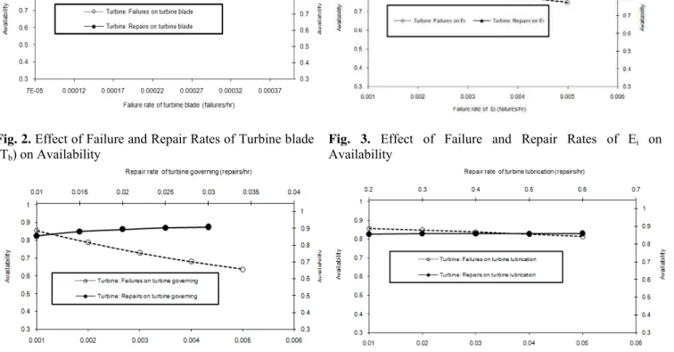
The availability simulation model (Av.) is used to predict the availability/performance of power generation system for known input values of failure and repair rates of its subsystems. The appropriate failure and repair rates of various subsystems of power generation system are taken from the literature/maintenance history sheets and through the discussions with the plant personnel of thermal power plant. Fig. 2 to 6 reveals the effect of baseline failure / repair rates (λ1=0.00007, µ1=0.0025,

λ2=0.001, µ2=0.01, λ3=0.01, µ3=0.2, λ4=0.001, µ4=0.01, λ5=0.0005, µ5=0.02) of Tb, Ei, Tl, Tg, Sj

respectively on availability simulation model (Av.) of the system. Fig. 2 represents that as the failure rates of Tb increases from 0.00007 to 0.00035 the availability decreases by about 8.7%. Similarly as

repair rates of Tb increases from 0.0025 to 0.0045, the availability increases by about 1.07%. Fig. 3

shows that as the failure rates of Ei increases from 0.001 to 0.005 the availability decreases by about

12.3%. Similarly as repair rates of Ei increases from 0.01 to 0.05, the availability increases by about

1.04%. Fig. 4 represents as the failure rates of Tg increases from 0.001 to 0.005 the availability

decreases by about 25.4%. Similarly as repair rates of Tg increases from 0.010 to 0.030, the availability

increases by about 6.04%. Fig. 5 shows that as the failure rates of Tl increases from 0.01 to 0.05 the

availability decreases by about 4.97%. Similarly as repair rates of Tl increases from 0.2 to 0.6, the

availability increases by about 0.42%. Fig. 6 represents as the failure rates of Sj increases from 0.0005

to 0.0025 the availability decreases by about 7.88%. Similarly as repair rates of Sj increases from 0.02

to 0.06, the availability increases by about 1.44%. Accordingly, maintenance decisions can be made for

3

j g l i bETTS

T

j g l i bETTS

T

j g l bETTS

T 1

j g l bETTS

T ₁

j g l i bETTS

t j g l i bETtS

T j g l i bETTs

T j g l i bETtS

T

j g l i bEtTS

T j g l i beTTS

T j g l i bETTs

T j g l i bETTS

t

j g l bETTS

t 1

j g l bETTs

T 1 j g l i beTTS

T

j g l bETtS

T 1

j g l bEtTS

T 1

j g l bETTS

t ₁

j g l bETTs

T ₁

j g l bETtS

T ₁

j g l beTTS

(6)

various subsystems keeping in view the repair criticality and we may select the best possible combinations of failure and repair rates.

Fig. 2. Effect of Failure and Repair Rates of Turbine blade

(Tb) on Availability

Fig. 3. Effect of Failure and Repair Rates of Ei on

Availability

Fig. 4. Effect of Failure and Repair Rates of Turbine

governing (Tg) on Availability

Fig. 5. Effect of Failure and Repair Rates of Turbine

lubrication (Tl) on Availability

Fig. 6. Effect of Failure and Repair Rates of Sj subsystem on Availability

Table 1

Optimum values of failure and repair rates of various subsystems of power generation system for maximum availability

S. No. Subsystem Failure rates (λi) Repair rates (µi) Maximum Availability

1. Turbine blade λ1=0.00007 µ1=0.0045 86.48 %

2. Ei subsystem λ2 = 0.001 µ2 =0.05 86.45 %

3. Turbine governing λ3 = 0.001 µ3 = 0.030 90.73 %

4. Turbine lubrication λ4 = 0.01 µ4 = 0.6 85.92 %

5. Sj subsystem λ5 = 0.0005 µ5 = 0.06 86.79%

(7)

4. Conclusions

The availability simulation model (Av.), for Power generation system has been developed with the help of mathematical modeling using probabilistic approach. The decision tables are also developed and shown in the form of graphs (Figs. 2-6). These figures facilitate the maintenance decisions to be made at critical points where repair priority should be given to some particular subsystem of power generation system. Fig. 4 clearly indicates that the Tg subsystem is most critical as far as maintenance aspect is concerned.

Therefore, it should be given top priority as the effect of its failure and repair rates on the unit availability is much higher than that of other sub-systems. While Fig. 5 shows Tl subsystem is found to be least sensitive.

Therefore, on the basis of repair rates, the maintenance priority should be given as per following order: 1) Turbine governing (Tg)

2) Turbine blade (Tb)

3) Ei: Condenser evacuation (E1), Regenerative subsystem (E2)

4) Sj: Seal oil system (S1), Generator cooling (S2)

5) Tl: Turbine lubrication

The optimum values of failure and repair rates for maximum availability of various subsystems of power generation system can be determined also shown in Table 1.

References

Arora, N., & Kumar, D. (1997). Stochastic analysis and maintenance planning of the ash handling system in the thermal power plant. Microelectronics Reliability, 37 (5), 819-824.

Arora, N., & Kumar, D. (1997). Availability analysis of steam and power generation systems in the thermal power plant. Microelectronics Reliability, 37 (5), 795-799.

American National Standards Institute. (1987). IEEE Std. 762 definitions for use in reporting electric generating unit reliability, availability and productivity. New York: The Institute of Electrical and Electronics Engineers, 7-12.

Balaguruswamy, E. (1984). Reliability Engineering. Tata McGraw Hill: New Delhi.

Barabady, J., & Kumar, U. (2007). Availability allocation through importance measures. International

journal of quality & reliability management, 24(6), 643-657.

Barabady, J., & Kumar, U. (2008). Reliability analysis of mining equipment: A case study of a crushing plant at jajram bauxite mine in Iran. Reliability Engineering and System Safety, 93 (4), 647-653.

Butler, R.W. (1986A). An abstract language for specifying Markov reliability models. IEEE Transaction on

Reliability, R35; 595-602.

Ciardo, G., Muppala, J., & Trivedi, K. (1989). Stochastic petri net package. In: Proceeding of the 3rd International workshop on Petri nets and performance models, Kyoto, Japan, 142-151.

Eti, M., Ogaji., S, & Probert S. (2007). Integrating reliability, availability, maintainability and supportability with risk analysis for improved operation of the AFAM thermal power-station. Applied Energy, 84(12), 202-221.

Ebeling, C. (2008). An Introduction to Reliability and Maintainability Engineering, 10th ed., Tata McGraw-Hill, New Delhi, India.

Vatn, J. and Aven, T. (2010). An approach to maintenance optimization where safety issues are important.

Reliability Engineering and System Safety, 4(3), 58-63.

Kaushik, S., & Singh, I.P. (1994). Reliability analysis of the feed water system in a thermal power plant.

Microelectronics Reliability, 34 (4), 757-759.

Kiureghian, A.D., & Ditlevson, O.D. (2007). Availability, Reliability & downtime of system with repairable components. Reliability Engineering and System Safety, 92(2), 66-72.

Koren, J.M., & Gaertner, J. (1987). CAFTA: A fault tree analysis tool designed for PSA. Proceeding of probabilistic safety assessment and risk management, PSA, Zurich, Switzerland, 588-592.

Kumar, D., Singh, J., & Singh, I.P. (1988). Availability of the feeding system in the sugar industry.

Microelectronics Reliability, 28, 867-871.

Kumar, D., Singh, J., & Singh, I.P. (1988). Reliability analysis of the feeding system in the paper industry.

(8)

Kumar, D., & Singh, J. (1989). Availability of a Washing System in the Paper Industry. Microelectronics

Reliability, 29, 775-778.

Lim, T.J., & Chang, H.K. (2000), Analysis of system reliability with dependent repair models; IEEE

Transaction on Reliability, 49(2), 153-62.

Mishra, R C., & Pathak, K. (2002). Maintenance Engineering and Management, Prentice Hall & India Pvt Ltd; New Delhi.

Purbolaksono, J. et. al (2010). Failure case studies of SA213-T22 steel tubes of boiler through computer simulations. Journal of Loss Prevention in theProcess Industries, 23 (1), 98-105.

Rahman, M.M., Purbolaksono, J., & Ahmad, J. (2010). Root cause failure analysis of a division wall superheater tube of a coal-fired power station. Engineering Failure Analysis, 17 (6), 1490-1494.

Samrout, M., Yalaoui, F., Châtelet, E., & Chebbo, N. (2005). Few methods to minimize the preventive maintenance cost of series-parallel systems using ant colony optimization. Reliability Engineering and

system safety, 89(3); 346-54.

Sharma, A.K. (1994). Reliability analysis of various complex systems in thermal power station, M.Tech Thesis, Kurukshetra University (REC Kurukshetra), Haryana, India.

Shu, L. et. al (2005). Functional reliability simulation for a power- station’s steam-turbine. Applied Energy, 80(1), 61-66.

Srinath, L. S. (1994). Reliability Engineering. 3rd edition, New Delhi, India. East-West Press Pvt. Ltd. Woo, Thomas G. (1980). Reliability analysis of a fluidized-bed boiler for a coal-fueled power plant. IEEE

Transactions on Reliability, 29 (5), 422-424.

Wolstenholme, L. C. (1999). Reliability modeling – a statistical approach. Chapman & Hall; CRC.

Appendix

To solve the Eq. (22) to Eq. (42) a computer program on MATLAB as given below can also be used to get the value of availability simulation model (AV.).

format long

global lambda1 lambda2 lambda3 lambda4 lambda5 lambda6 mu1 mu2 mu3 mu4 mu5 mu6 k1 k2 k3 k4 k5

lambda1= assign value; lambda2= assign value; lambda3= assign value; lambda4= assign value; lambda5= assign value; lambda6= assign value;

mu1= assign value; mu2= assign value; mu3= assign value; mu4= assign value; mu5= assign value; mu6= assign value;

k1=lambda1/mu1; k2=lambda2/mu2; k3=lambda3/mu3; k4=lambda4/mu4; k5=lambda5/mu5; A=[ lambda6+mu3 0 -mu6*k1 ; 0 lambda3+mu2 -mu3 ; -lambda6 -lambda3 mu3+mu6]; B=[lambda3; lambda2; 0];

s=inv(A)*B; k=sum(s); n=1+k;

l4=s(1,1); l10=s(2,1); l15=s(3,1);

g=n+k1+k4+k5+((k1)*(l4))+((k2)*(l4))+((k3)*(l4))+((k4)*(l4))+((k5)*(l4))+((k1)*(l10))+((k2)*(l10)) +((k4)*(l10))+((k5)*(l10))+((k1)*(l15))+((k2)*(l15))+((k3)*(l15))+((k4)*(l15))+((k5)*(l15));