A Work Project carried out on the Business and Public Policy Major, presented as part of the requirements for the Award of a Master’s Degree in Management from the
NOVA – School of Business and Economics.
What are the effects of mass retailers on Lisbon
’s
Municipal Markets?
A
NAD
UARTEA
BREU ES
ILVA,
#744
UNDER THE SUPERVISION OF:PROFESSOR SOFIA FRANCO
What are the effects of mass retailers on Lisbon’s
Municipal Markets?
A
BSTRACTThe primary purpose of this research is to analyze the impact of mass retailers on Municipal Markets in the city of Lisboa between 2004 and 2009. A Prais-Winsten regression with specific panel AR(1) and PCSEs was used to estimate the model. The findings reveal that, on average, an increase of 1 supermarket per km2within the “Freguesia” where the municipal
market is located leads to a decrease of 3.48% in the occupation rates while an increase of 0.1 hypermarkets per km2 leads to a decrease of 5.62% if it is located within the “Freguesia” and of
10.10% if it is located in the adjacent ones.
1. Introduction
Non-traditional food retailers have changed the retail business landscape around the world. The rapid growth of alternative retail formats has transformed not only the competitive structure of the industry, but also the way in which consumers shop. This trend has increased the competitive pressure on smaller stores which compete in a “monopolistic” framework within their neighborhoods. The grocery industry shifted from an industry dominated by small retailers serving local markets to one characterized by mass retailers.
In Portugal, super and hypermarkets have grown noticeably in the last decades. According to Nielsen (2005) the market share of mass retailers more than doubled between 1985 and 2004 while the market share of traditional food retailers decreased by 27% during the same period. As supermarkets spread and their market share grew the market share of traditional retailers declined.
The purpose of this study is to examine the impact of supermarkets and hypermarkets on the sales of a particular form of traditional retailer – Municipal Markets. Although these markets can be found in any city of any size in Portugal, the analysis is focused only in the city of Lisboa where municipal markets are under “Câmara Municipal de Lisboa” (CML) management. It uses a Prais-Winsten regression with specific panel AR(1) and PCSEs to analyze the impact of supermarkets and hypermarkets on 29 municipal markets in the city of Lisboa between 2004 and 2009. To date, no studies have quantified the magnitude of the effect of mass retailers on the business activity of this type of traditional retailers in Portugal. In this way, this study makes a contribution to the literature.
sellers working individually, owning their own stands and sharing common areas and common resources. Municipal markets sell mostly perishable products such as fruit, vegetables, meat, fish and flowers but some also sell garments and jewelry.
At their beginning municipal markets had a very important role providing the convenience of a one way shopping trip since most urban residents did not own a car. Moreover these places offered lower prices for most of the goods the consumer needed since they gathered a large amount of sellers in just one place. So competition was very fierce. In addition they also functioned as a social place where people could meet and chat about the latest news. They also provided positive spillovers externalities to adjacent areas creating business opportunities in the housing market by increasing housing rents and housing prices.
As households’ income increased over time and the means of transportation became
more sophisticated consumers were not restricted to shopping trips within their residential areas. Consumers also became more demanding towards their shopping experience. The rise of supermarkets, hypermarkets and convenience neighborhood chain stores helped fulfill some of the new preferences of urban consumers.
As the market share of mass retailers increased, concerns have emerged that large grocers could use their lower cost structure, advantages in marketing, and store design to increase their retailer market power and discourage competition. On the other hand, the effect of increased competition from non-traditional retailers could have forced traditional retailers to change and adopt new food-pricing strategies. Yet, this has not occurred and municipal markets are currently experiencing a decrease in their demand. It is therefore necessary to understand whether mass retailers prove a source of competition to municipal markets and if so measure the magnitude of their impact on this type of traditional retailers. Only then policies can be designed to help increase the competitiveness of municipal markets in a market dominated by mass retailers.
Previous studies (Borraz et al, 2009; Kaliappan et al, 2008; Suryadarma et al, 2007; among others) documented the effect of large scale stores on small retailers’ sales and the probability of survival in other countries. In sum, there is clear evidence that the entry and expansion of mass retailers have impact on the existing small retailers. However the sign and the amplitude of the impact of a large retailer on local retailers depend on various aspects such as the type of local retail businesses, the proximity between the business, the size and competitiveness of local retail businesses.
The literature on the impact of supermarkets’ entry is tied to specific contexts and therefore could not be applied to different situations. Moreover the lack of findings directly relevant to Portugal also provides further justification for this research.
The paper proceeds as follows. The next section provides a brief summary on relevant literature concerning the topic this paper analyzes. Then, the dataset and the methodology are presented. Section 5 discusses the results and Section 6 concludes.
2. Literature Review
This section provides an overview of the related literature available concerning the impact of the supermarkets’ entry within the food retailing industry. This review focus
on four major subjects and on two methodologies (survey and regression analysis).
Impact of supermarkets’ entry on traditional retail stores
Borraz et al. (2009) used a panel data analysis to study the impact of supermarket’s
entry on small grocery retailers in 18 urban areas of Montevideo, Uruguay, between 1998 and 2007. They estimated the grocery survival probabilities through a panel logit model using the conditional maximum likelihood estimator. Results indicated that the probability of survival of small retailers decreases as the number of supermarkets, or their total area, increases. On average, the entry of one supermarket in a small grocery store’s neighborhood increased its chance of exiting the market in that year by 1.2%.
between hypermarkets and local retailers in terms of store attributes, products offered and prices. Meanwhile those retailers who agreed to a certain extent with the presence of hypermarkets generally are those who are doing complementary business.
Suryadarma et al. (2007) measured the impact of supermarkets on traditional market traders in Indonesia’s urban centers using both in-depth interviews and difference-in-difference analysis. On average, traders have experienced a decline in their business over the past three years. The in-depth interviews revealed that the main causes of this decline were the weakened purchasing power of their customers due to the fuel price increases, the increased competition with street vendors who occupy the areas surrounding the markets and the existence of supermarkets. Suryadarma et al. (2007) found evidence that traditional markets located near supermarkets are more adversely affected than those further away. However, this was mainly due to the weak competitiveness of traditional retailers. The quantitative impact analysis found mixed statistical results for various performance indicators of traditional markets, such as profits, earnings, and employee numbers. Only the number of employees is affected by the presence of supermarkets. Traditional retailers are willing to hire more employees the farther they are located from the supermarkets. While there is evidence of retailers that have gone out of business, reasons are more complex than just the entry of supermarkets. Most exits are related to internal market and personal problems. In addition, shoppers who sell mainly to non-households and have maintained a good relationship with customers over a long period are more likely to stay in business.
supercenter or warehouse club decreases grocery sales in neighboring counties; The entry of a supercenter or warehouse club decreases the number of small grocery retailers in immediate non-metropolitan and in adjacent counties. Linear regressions were estimated to determine the effects of entry by large warehouse and supercenter stores on sales and on the change in the number of small supermarkets. Spatial regimes or groupings of similar counties were used. Therefore, two types of spatial effects were tested in both models: spatial heterogeneity and dependence. Results suggested that warehouse and supercenter stores had a significant and large effect on the change in grocery sales and the exit of small supermarkets operating at the country level. Only the third hypothesis, that warehouse club and supercenter store entries decrease the number of small supermarkets in non-metropolitan areas, has been proven incorrect.
Impact of Wal-Mart’s entry into the traditional supermarket industry
Singh et al. (2004) provided an empirical study on the impact of a Wal-Mart supercenter entry on sales of a traditional supermarket store located in the East coast of the U.S. By using a frequent shopper database from this store they developed a joint model of inter-purchase time and basket size and allowed for a structural break at the time of competitive entry. The model allowed them to evaluate the impact of Wal-Mart on household store visit frequency and basket size, while allowing for consumer heterogeneity. They investigated the shopping and demographic characteristics of the consumers that are most likely to shift purchases to Wal-Mart. Their results showed that the incumbent store lost 17% volume following Wal-Mart’s entry amounting to a quarter million dollars in monthly revenue. Decomposing the lost sales into components attributed to store visits and in-store expenditures, they found that the majority of the losses were due to fewer store visits with a much smaller impact on basket sizes. Also distance to the store explains little of the variation in household heterogeneity. Households that responded to Wal-Mart are likely to be large basket consumers and to have an infant and pet and are more likely to be weekend shoppers. On the other hand, households that spent a large proportion of their grocery expenditures on fresh produce, seafood, and home meal replacement items were less likely to defect to Wal-Mart.
Consumer demographics and retail format choice
Carpenter and Moore (2006) provided a general understanding of grocery consumer’s retail format choice in the U.S. market by identifying the demographic
insights. With regard to store attributes, cleanliness is the most important attribute regardless of format. The price competitiveness appeared to be most important among shoppers in the traditional supermarket format and the supercenter format. Surprisingly, price competitiveness did not rank among the top five attributes for occasional shoppers in the supercenter format or the specialty grocery format and ranked only fifth among these shoppers for the warehouse format. While many assert that the grocery industry is strongly driven by price competitiveness, their results suggested that product selection and courtesy of personnel are also very important in determining format choice.
Price and Concentration
Lamm (1981) presented new evidence on the nature of the price structure relationship for the food retailing industry using individual market shares and 1-firm through 4-firm concentration ratios as structure measures. The analysis is based on a simple food price determination model estimated using a pooled cross section and time series data set consisting of 72 observations for 18 urban areas from 1974 to 1977. The basic dependent variable included in the study is the price of an approximately homogenous food market basket for a family of 4. The study shows that the choice of a market structure measure is important for determining the nature of the structure-price relationship in the food retailing industry. In particular, the equal weight scheme inherent in the use of the concentration ratio is found to mask some of the important aspects of firm-share distribution. Growth in 3-firm concentration causes food prices to rise with the second largest firm’s share has an offsetting effect, however. From a policy
In sum, even though there are not many comprehensive studies on the impact of mass retailers on traditional retailers, there is clear evidence that the entry and expansion of mass retailers will exert impacts on the existing small businesses. Whether the impact is positive or negative, small or huge, depends on various factors such as the type of local retail businesses, the proximity of existing business and the new entrant, the size and competitiveness of local retail businesses.
3. Data Description
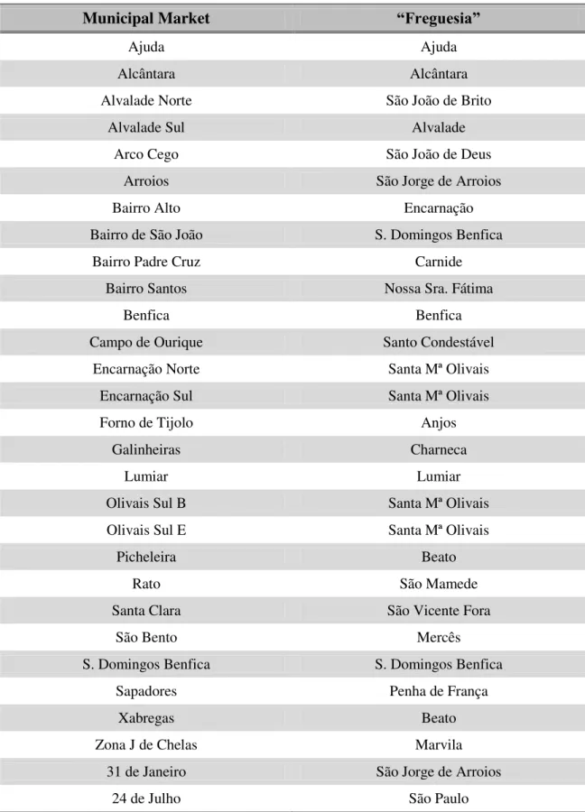
This section describes how the dataset used in this analysis was built. The unit of analysis is the municipal market and the period of analysis comprises the years between 2004 and 2009. Therefore there are 29 group variables corresponding to the 29 municipal markets and 6 time variables corresponding to the years 2004, 2005, 2006, 2007, 2008 and 2009.
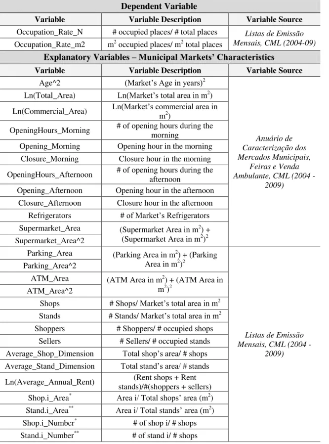
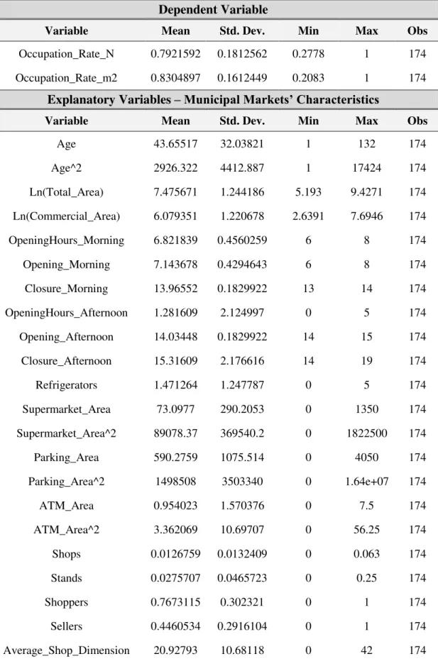
All variables except for those related with municipal markets’ characteristics are measured at the “Freguesia” level. We excluded from the analysis all “Freguesias” that did not have a municipal market. In total we collected data for 23 “Freguesias” of Lisboa. A list of the various types of variables used in this analysis is exhibited in Table 1 in Appendix A and a description of the sample is exhibited in Table 2 in Appendix B.
3.1. Dependent Variable
some of the sellers have already retired or passed away which makes it more difficult to put together a dataset on the amount of sales and number of sellers operating in each municipal market over time. We have thus used a proxy to capture these sellers business performance over time.
Competition within each market is very high and since there are many sellers with similar cost structures selling very similar products, we can say that within each market competition resembles that of monopolistic competition. In a monopolistic competitive market the existence of economic profits will attract new entrants until each firm’s economic profit is zero. This implies a very particular geometrical relationship. Both the demand and the average cost curves must be tangent to each other.
Sometimes, however, firms are operating below the tangency point, earning negative profits. This happens because if above average variable cost curve firms could avoid bigger losses. Firms are still able to cover part of their fixed costs. This situation could not however be sustained forever. If firms continue operating below the tangency point in the long run they will exit the market. This suggests that municipal markets’ occupation could be used as a proxy for its business activity. The occupation rate is measured as a percentage of the places – shops and stands - occupied in each year. It can be measured in terms of number of occupied places or in terms of occupied area.
result, it was necessary to build a more consistent and clean dataset which was very time consuming. In particular, variables were grouped according to the following criteria: total number/area of shops/stands in each Municipal Market in each year; total number/area of occupied shops/stands in each Municipal Market in each year; total number of shoppers/sellers in each Municipal Market in each year; the average annual rent paid by the shoppers/sellers to CML in each Municipal Market in each year; and the same for each product category.
3.2. Independent Variables
There are several factors that can influence occupation rates. We included in our analysis several variables that capture the competitive environment within the influence area of each municipal market. We also used variables that captured the characteristics of municipal markets, the neighborhood where the municipal market is located and the characteristics of local residents. Table 1 in Appendix A presents all the variables used.
Variables on the municipal market’s characteristics were built with information from the “Anuário de Caracterização dos Mercados Municipais” and from “Listas de Emissão Mensais”, both provided by CML. Variables on the trade environment of each “Freguesia” came from “Recenseamento dos Estabelecimentos de Comércio a Retalho e Restauração e Bebidas da Cidade de Lisboa” also provided by CML.
Demographic variables were computed using data from the 2001 and 2011 Censos. The 2001 Censos was used to characterize population in each “Freguesia” from 2004 until 2006. The 2011 Censos was used to characterize population from 2007 until 2009. Although income is a relevant variable as the studies in the literature review show, this data is only available at the “Concelho”. Instead one used education as a proxy. One expects that households with higher education have higher income levels on average.
4. Model Specification
This analysis rests on the development of an econometric model for municipal markets’ occupation rates. This section briefly describes our econometric model specification. For further details on the model specification please see Appendix B.
A key question is whether one should use the fixed effects (FE) estimator or the random effects (RE) estimator. A more conservative approach is to assume that the unobserved effect is correlated with the explanatory variables and use the FE estimator.
Our Hausman statistic is relatively small (13.60 with p-value = 0.1919) which implies that the differences between the coefficients are not big enough to be significance.1 So, one fails to reject (with 5% significance) the null hypothesis. Therefore, RE should be used. In particular we used the sigmamore version. We also tested for serially correlated errors using the Lagrange multiplier (LM) test.2 After running the Lagrange multiplier test (statistic = 2.89; p-value = 0.0892) and taking into
1 The result of the Hausman test indicates that this research should use a RE model instead of a FE one.
The Hausman test checks a more efficient model against a less efficient but consistent model to make
sure that the more efficient one also gives consistent results. The bigger the difference, the higher the
Hausman statistic.
2 The LM test helps to decide between a RE regression and a simple OLS regression. The null hypothesis
consideration a 10% significance level we did not fail to reject the null that and conclude again that RE is appropriate.
The Prais-Winsten Estimation is a procedure that accounts for serial correlation of type AR(1). However, because we are interested on first-order autocorrelation within panels with panel specific AR(1) coefficients, a panel specific AR(1) should be computed instead of the usual AR(1). Therefore, we have employed the following model specification (Prais-Winsten regression with specific panel AR(1) and PCSEs):
∑ , (1)
where i =1,2,..., N refers to a cross-sectional unit; t =1,2,..., T refers to a time period and k =1,2,..., K refers to a specific explanatory variable. Thus, yit and xit refer respectively to the dependent and independent variables for unit i and time t; is a random error and β0 and βk refer, respectively, to the intercept and the slope parameters. Moreover we can denote the NT×NT variance-covariance matrix of the errors with typical element
by . Equation 1 was estimated using the statistical package STATA.
5. Results
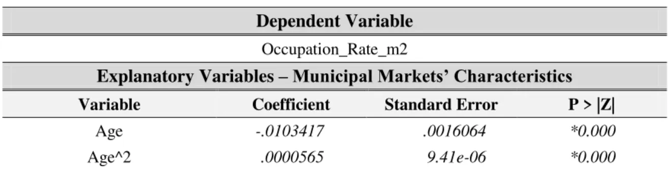
This section presents and discusses the results. Table 1 presents the estimated coefficients and correspondent standard errors and p-values for all variables.
Table 1: Estimation Results
Dependent Variable
Occupation_Rate_m2
Explanatory Variables –Municipal Markets’ Characteristics
Variable Coefficient Standard Error P > |Z| Age -.0103417 .0016064 *0.000
Ln(Total_Area) .099945 .0175594 *0.000
Closure_Afternoon .0599693 .0108711 *0.000
Supermarket_Area -.0001823 .0001782 0.306
Supermarket_Area^2 1.72e-07 1.72e-07 0.319
Parking_Area -.0006162 .0000671 *0.000
Parking_Area^2 2.29e-07 2.79e-08 *0.000
ATM_Area .1043597 .0296789 *0.000
ATM_Area^2 -.03247 .0072967 *0.000
Stands 3.985119 .4224504 *0.000
Sellers .3729489 .0801037 *0.000
Average_Shop_Dimension .0040441 .0018752 **0.031
Average_Stand_Dimension -.0773487 .0155105 *0.000
Ln(Average_Annual_Rent) .178409 .022897 *0.000
Explanatory Variables – Trade Environment
Variable Coefficient Standard Error P > |Z| FoodBeverage_Area 1.438681 1.191979 0.227
Explanatory Variables – Competition
Variable Coefficient Standard Error P > |Z|
Mini .0041492 .00471 0.378
Super -.034823 .0097261 *0.000
Hyper -.562471 .2477272 **0.023
Mini_Adj .0096856 .0093362 0.300
Super_Adj -.0385587 .0311815 0.216
Hyper_Adj -1.009818 .3492053 *0.004
Explanatory Variables – Demographics
Variable Coefficient Standard Error P > |Z| Population .0000142 4.10e-06 *0.001
Average_Age -.0277336 .0097489 *0.004
Education_HigherEd -.1799537 .1340959 0.180
Ln(Area) .1073502 .0250335 *0.000
Intercept
Variable Coefficient Standard Error P > |Z| Intercept -2.447124 .4054661 *0.000
Statistics
Number of Observations 174
Group Variable (N=29) Mercado_Municipal
Time Variable (T=6) Year
R-squared 0.9492
About 95 percent of the variability in occupation rates is accounted by the model. As such our model has a good explanatory power. All variables in the model are statistical significant except the area of supermarkets within the market’s building, food and beverage stores’ area, percentage of population with higher education, minimarkets within the “Freguesia” and mini and supermarkets within adjacent “Freguesias”.
The total area of the municipal market is a statistical significant factor affecting occupation rates. On average, an increase of 10 m2 causes an increase of 1.00% in the occupation rates. Opening and closing hours are also important explanatory variables. A wider schedule would allow municipal markets to target other customers apart from retired people, housemaids and free-schedule workers. The coefficient on the afternoon closing timing is positive and statistically significant at the 1% level. An increase of 1 hour causes an increase of 6.00% in the occupation rate on average.
The age of the building where the municipal market sits is also a relevant factor and it can proxy for the maintenance conditions of the market infrastructure. Older commercial buildings tend to have a less attractive shopping environment if not maintained properly. The sign associated with this variable is negative until 183 years being therefore positive. The positive impact could be due to historical reasons. From a certain age buildings start to be visited as monuments and customers go there not to buy perishable products but to admire the building. However once there they might shop.
do not live near the market and/or do not have time to weekly shopping trips and therefore buy in bulk.
The effect of ATMs is only positive until 3.214 m2 being therefore negative. Since only one municipal market as an ATM area bigger than 4 m2 we should only take into consideration the function within [0; 3.214]. In this region the ATM area has always a positive effect. It is also possible to conclude that the first ATM is more important than the remaining ones, having a bigger impact.
Occupation rates also increase as the average number of stands per km2 increases. An increase of 1 stand per km2 causes an increase of 0.40% in the occupation rate on average. If the municipal market has more space dedicated to other activities it has necessarily less space dedicated to stands which is its core business and distinctive advantage. Less space dedicated to it will therefore keep consumers away.
The coefficient on the average number of sellers per stand is positive and statistically significant at the 1% level. An increase of 0.1 seller per stand leads to an increase of 3.73% in the occupation rate on average (this explanatory variable only varies between 0 - no stands - and 1 - one stand per seller; any number between means more than one stand per seller). Less stands per seller means higher competition and therefore lower prices. Less stands per seller also means less probability of dumping.
The average size of shops and stands also impact the occupation rates. On average, an increase of the shop’s average size in 1 m2 will lead to an increase of 0.40% in the
occupation rates. This means that in general, municipal markets with higher shops have higher occupations rates. On the other hand, an increase of the stand’s average size in 1
The coefficient on the logarithm of the average annual rent is positive and statistically significant at the 1% level. An increase of 10€ causes an increase of 1.78% in the occupation rate on average. This result seems counterintuitive at first glance but it is not. Sellers usually tend to work in order to meet their cost’s obligations and in order to save some money that can be understood as their salaries. If they have to pay higher rents they will have to make an effort to improve their performance which will attract more customers and therefore new sellers.
The number of minimarkets within the “Freguesia” does not impact occupation rates. This retail stores (< 200 m2) tend to be family business replicating a lot of municipal markets’ characteristics. Therefore they tend to not have an impact on municipal markets. The number of mini and supermarkets within the adjacent
“Freguesias” also does not impact occupation rates. These two formats of retail are well spread throughout the city of Lisboa (on average each “Freguesia” has 4 minimarkets and 1 supermarket). Then, one does not have to go to the neighborhoods to find one of them, explaining the level of significance of those two variables.
The coefficient on supermarkets per km2 within the “Freguesia” is negative and statistically significant at the 1% level. An increase of 1 supermarket per km2 causes a decrease of 3.48% in the occupation rate on average. Since supermarkets can offer some features that municipal markets cannot such as lower prices, its presence tend to affect negatively the occupation rates of municipal markets.
also makes sense since households tend to choose this format for high volume purchases, needing to use their car. On average, an increase of 0.1 hypermarkets per km2 within the “Freguesia” leads to a decrease of 5.62% in the occupation rates while an increase of 0.1 hypermarkets per km2 within the adjacent “Freguesias” causes a decrease of 10.10% in the occupation rates.
Population density is a statistically significant factor affecting occupation rates. For every 1000 person increase per km2, occupation rates increase 1.42%. Average age of urban residents is also relevant. An increase of 1 year causes a decrease of 2.77% in the occupation rate on average. Older people tend to have lower purchasing power leading to lower occupation rates.
The coefficient on the percentage of the population with higher education is not statistically significant at the 10% level. High income people could afford to buy in municipal markets where prices tend to be higher. However as the level of education of the “Freguesia” residents increase, consumers may switch to other grocery outlets or may increase expenditures in the away-from home market. These two contradictory effects could explain the insignificance of the variable.
Results also show that the occupation rate increases as the size of the “Freguesia” in m2 increases. An increase of 10 m2 causes an increase of 1.07% in the occupation rate on average. Then, bigger “Freguesias” tend to have higher occupation rates.
6. Concluding Remarks
proxy for the municipal market business activity) of municipal markets located in Lisboa was analyzed. To accomplished this task, we employed a Prais-Winsten regression with specific panel AR(1) and PCSEs model specification. Data for this analysis cover annual time periods from 2004 to 2009 for 29 municipal markets within the city of Lisboa.
Our results suggest that super and hypermarkets have a negative impact on municipal markets’ occupation rates. Supermarkets within the “Freguesia” where the municipal market is located have impact while supermarkets in adjacent “Freguesias” do not. Hypermarkets regardless of their location have a negative impact on municipal markets. On average an increase of 1 supermarket per km2 leads to a decrease of 3.48% in the occupation rates while an increase of 0.1 hypermarkets per km2 leads to a decrease of 5.62% if it is located in the same “Freguesia” and a decrease of 10.10% if it is located in the adjacent ones.
What implications can we draw from this study? Municipal markets will face heightened competition from mass retailers such as hypermarkets and supermarkets like “Continente” and “Pingo Doce” and at the same time, but to a lesser degree, from minimarkets. To stabilize market share, municipal markets should make additional efforts to reduce prices and yet maintain profit margins. They should also try to engage in more aggressive differentiation strategies by offering greater variety of products and a wider schedule, advertising and investing in the shopping environment. Municipal markets should also try to lower their cost structure and improve their competitive position vis-à-vis mini and supermarkets in close proximity. That may imply take tougher stances in the negotiations of the infrastructure rents and utilities with CML.
products. Municipal markets’ have no conditions to compete with these formats. They should bet on their distinctive advantages like their locations within residential areas and their personalized and attentive service.
Municipal markets could also bet on their “social dimension”. They usually symbolize the “Freguesia” where they are located and they are therefore a reference of the neighborhood. “Unintentional monuments” and places of “memory and identity”, municipal markets can be unique places in the city of Lisboa. They should therefore be preserved as locations of solid social relations between residential populations, acting as “Living Monuments”. They could be marketed as historic amenities that give a flavor to the “Freguesia” and used as urban amenities to attract population into the city.
References
BASKER, Emek; NOEL, Michael. 2009. “The Evolving Food Chain: Competitive
Effects of Wal-Mart’s Entry into the Supermarket Industry”. Journal of Economics & Management Strategy, 18(4): 977 – 1009.
BORRAZ, Fernando; DUBRA, Juan; FERRÉS, Daniel; ZIPITRÍA, Leandro. 2009.
“Supermarket Entry and its effect on small stores in Montevideo, 1998 to 2007”.
CARPENTER, Jason M.; MOORE, Marguerite. 2006. “Consumer Demographics,
Store Attributes, and Retail Format Choice in the US Grocery Market”. International Journal of Retail & Distribution Management, 34(6): 434 – 452.
KALLIAPPAN, Shivee Ranjanee; ALAVI, Rokiah; ABDULLAH, Kalthom;
ZAKAULLAH, Muhammad Arif. 2008. “Liberalization of Retail Sector and the
LAMM, R. McFall. 1981. “Prices and Concentration in the Food Retailing Industry”.
The Journal of Industrial Economics, 30(1): 67 – 78.
MARTENS, Bobby; FLORAZ, Raymond J. G. M.; DOOLEY, Frank. 2005. “The
Effect of Entry by Supercenter and Warehouse Club Retailers on Grocery Sales and Small Supermarkets: A Spatial Analysis”. American Agricultural Economics Association Annual Meeting, July 24 – 27, 2005.
SINGH, Vishal P.; HANSEN, Karsten T.; BLATTBERG, Robert C. 2004. “Impact of
Wal-Mart Supercenter on a Traditional Supermarket: An Empirical Investigation”.
SURYADARMA, Daniel; POESORO, Adri; BUDIYATI, Sri; ROSFADHILA,
Meuthia; Akhmadi. 2007. Impact of Supermarkets on Traditional Markets and Retailers
in Indonesia’s Urban Centers. Jakarta: SMERU Research Institute
VALENTE, Luísa; MOLEIRO, Ascenção; SABINO, Cristina; LOPES, Carla;
CARRETO, António. 2007. Anuário de Caracterização dos Mercados Municipais, Feiras e Venda Ambulante. Lisboa: Câmara Municipal de Lisboa
VALENTE, Luísa; MOLEIRO, Ascenção; GOMES, Tiago. 2004. Anuário de
Caracterização dos Mercados Municipais, Feiras e Venda Ambulante. Lisboa: CML
WOOLDRIDGE, Jeffrey M. 2002. Introductory Econometrics: A Modern Approach.
UK: Amazon
Listas de Emissão Mensal 2009, 2008, 2007, 2006, 2005, 2004. Lisboa: CML, DMAU, DMF
A
PPENDIX ATable 1: Summary of the variables computed for the econometric model
Dependent Variable
Variable Variable Description Variable Source Occupation_Rate_N # occupied places/ # total places Listas de Emissão
Mensais, CML (2004-09)
Occupation_Rate_m2 m2 occupied places/ m2 total places
Explanatory Variables –Municipal Markets’ Characteristics
Variable Variable Description Variable Source Age^2 (Market’s Age in years)2
Anuário de Caracterização dos Mercados Municipais,
Feiras e Venda Ambulante, CML (2004 -
2009)
Ln(Total_Area) Ln(Market’s total area in m2)
Ln(Commercial_Area) Ln(Market’s commercial area in m2)
OpeningHours_Morning # of opening hours during the morning
Opening_Morning Opening hour in the morning Closure_Morning Closure hour in the morning
OpeningHours_Afternoon # of opening hours during the afternoon
Opening_Afternoon Opening hour in the afternoon Closure_Afternoon Closure hour in the afternoon
Refrigerators # of Market’s Refrigerators Supermarket_Area (Supermarket Area in m2) +
(Supermarket Area in m2)2
Supermarket_Area^2
Parking_Area (Parking Area in m2) + (Parking
Area in m2)2
Listas de Emissão Mensais, CML (2004 -
2009)
Parking_Area^2
ATM_Area (ATM Area in m2) + (ATM Area in
m2)2
ATM_Area^2
Shops # Shops/ Market’s total area in m2
Stands # Stands/ Market’s total area in m2
Shoppers # Shoppers/ # occupied shops Sellers # Sellers/ # occupied stands Average_Shop_Dimension Total shop’s area/ # shops Average_Stand_Dimension Total stand’s area/ # stands
Ln(Average_Annual_Rent) stands)/#(shoppers + sellers) (Rent shops + Rent
Shop.i_Area* Area i/ Total shops’ area (m2)
Stand.i_Area** Area i/ Total stands’ area (m2)
Explanatory Variables – Trade Environment
Variable Variable Description Variable Source Ln(Category_i)*** Ln(Area of Category i)
Recenseamento dos estabelecimentos de comércio a retalho e restauração e bebidas da
cidade de Lisboa. CML (2004 - 2009)
Ln(SubCategory_i)**** Ln(Area of Category i)
Category.i_Area*** Area Category i/ Area of
“Freguesia”
Subcategory.i_Area**** Area Subcategory i/ Area of
“Freguesia”
Explanatory Variables – Competition
Variable Variable Description Variable Source Mini # Minimarkets/ Supermarkets/
Hypermarkets per km2 in the
“Freguesia”
Recenseamento dos estabelecimentos de comércio a retalho e restauração e bebidas da
cidade de Lisboa. CML (2004 - 2009)
Super Hyper
Mini_Adj # Minimarkets/ Supermarkets/ Hypermarkets per km2 in the
adjacent “Freguesia”
Super_Adj Hyper_Adj
Explanatory Variables – Demographics
Variable Variable Description Variable Source Population # inhabitants per km2
Censos 2001 and 2011
Average_Age Weighted average of the midpoints of the age’s intervals
Education_None Percentage of the inhabitants with none education
Education_Basics1 Percentage of the inhabitants with 1st cycle of basics completed
Education_Basics2 Percentage of the inhabitants with 2nd cycle of basics completed
Education_Basics3 Percentage of the inhabitants with 3rd cycle of basics completed
Education_Secondary Percentage of the inhabitants with secondary completed
Education_PostSecondary Percentage of the inhabitants with a post-secondary course completed
Education_HigherEd Percentage of the inhabitants with a higher education course completed Average_N.Persons_Family Average # of persons per family
Ln(Area) Ln(“Freguesia’s” Area)
*i(shop) = Talhos; Criação e Caça; Leitão Assado e Churrasqueira; Fumados e Queijos; Leite e Derivados; Padaria; Peixe Fresco; Produtos Hortofrutícolas; Congelados; Mercearia e Charcutaria; Artigos de Jardim e Flores; Drogarias; Artigos de Vestiário Diverso; Retrosarias e Bijuterias; Sapatarias e Reparação de Calçado; Material de Escritório e Papelarias; Estabelecimentos de Restauração e Bebidas; Lavandarias
**i(stand) = Produtos Hortofrutícolas; Produtos Frutícolas; Peixe Fresco; Criação e Caça; Leitão Assado e Churrasqueira; Fumados e Queijos; Mercearia e Charcutaria; Congelados; Padarias; Bolos; Artigos de Jardim e Flores; Artigos de Vestiário Diverso ***i(category) = Food retail stores; Non-food retail stores; Food and beverage
A
PPENDIXB
Table 1: Location of Municipal Markets within the City of Lisboa
Municipal Market “Freguesia”
Ajuda Ajuda
Alcântara Alcântara
Alvalade Norte São João de Brito
Alvalade Sul Alvalade
Arco Cego São João de Deus
Arroios São Jorge de Arroios
Bairro Alto Encarnação
Bairro de São João S. Domingos Benfica
Bairro Padre Cruz Carnide
Bairro Santos Nossa Sra. Fátima
Benfica Benfica
Campo de Ourique Santo Condestável Encarnação Norte Santa Mª Olivais
Encarnação Sul Santa Mª Olivais
Forno de Tijolo Anjos
Galinheiras Charneca
Lumiar Lumiar
Olivais Sul B Santa Mª Olivais
Olivais Sul E Santa Mª Olivais
Picheleira Beato
Rato São Mamede
Santa Clara São Vicente Fora
São Bento Mercês
S. Domingos Benfica S. Domingos Benfica
Sapadores Penha de França
Xabregas Beato
Zona J de Chelas Marvila
31 de Janeiro São Jorge de Arroios
Table 2: Summary Statistics of the variables
Dependent Variable
Variable Mean Std. Dev. Min Max Obs
Occupation_Rate_N 0.7921592 0.1812562 0.2778 1 174
Occupation_Rate_m2 0.8304897 0.1612449 0.2083 1 174
Explanatory Variables –Municipal Markets’ Characteristics
Variable Mean Std. Dev. Min Max Obs
Age 43.65517 32.03821 1 132 174
Age^2 2926.322 4412.887 1 17424 174
Ln(Total_Area) 7.475671 1.244186 5.193 9.4271 174
Ln(Commercial_Area) 6.079351 1.220678 2.6391 7.6946 174
OpeningHours_Morning 6.821839 0.4560259 6 8 174
Opening_Morning 7.143678 0.4294643 6 8 174
Closure_Morning 13.96552 0.1829922 13 14 174
OpeningHours_Afternoon 1.281609 2.124997 0 5 174
Opening_Afternoon 14.03448 0.1829922 14 15 174
Closure_Afternoon 15.31609 2.176616 14 19 174
Refrigerators 1.471264 1.247787 0 5 174
Supermarket_Area 73.0977 290.2053 0 1350 174
Supermarket_Area^2 89078.37 369540.2 0 1822500 174
Parking_Area 590.2759 1075.514 0 4050 174
Parking_Area^2 1498508 3503340 0 1.64e+07 174
ATM_Area 0.954023 1.570376 0 7.5 174
ATM_Area^2 3.362069 10.69707 0 56.25 174
Shops 0.0126759 0.0132409 0 0.063 174
Stands 0.0275707 0.0465723 0 0.25 174
Shoppers 0.7673115 0.302321 0 1 174
Sellers 0.4460534 0.2916104 0 1 174
Average_Stand_Dimension 2.121317 1.300889 0 5.0976 174
Ln(Average_Annual_Rent) 7.534873 0.5049589 5.5763 8.6263 174
Explanatory Variables – Trade Environment
Variable Mean Std. Dev. Min Max Obs
LN(FoodRetail) 8.351459 1.095967 5.9839 10.1764 174
LN(NonFoodRetail) 9.844152 1.015174 7.1164 11.1998 174
LN(FoodBeverage) 9.027209 0.8098071 7.1793 10.406 174
LN(SpecializedFoodRetail) 6.892741 0.7141495 4.9558 7.954 174
LN(NoSpecializedfoodRetail) 8.000292 1.293984 5.0499 10.1157 174
LN(PersonalUse) 7.874902 1.443676 3.912 10.0093 174
LN(HouseholdEquipment) 8.383504 1.064576 5.3936 10.1879 174
LN(HygieneHealth) 6.694903 0.9287661 4.3175 7.9572 174
LN(CultureLeisure) 7.499152 0.9915469 4.7958 9.3042 174
LN(OtherNonFoodRetail) 8.799995 1.189675 5.9243 10.2688 174
FoodRetail_Area 0.0027799 0.0016671 0.0006 0.0071 174
NonFoodRetail_Area 0.0163718 0.0155397 0.0007 0.0559 174
FoodBeverage_Area 0.007831 0.0112494 0.0008 0.0618 174
SpecializedFoodRetail_Area 0.0007914 0.0007702 0.0001 0.0043 174
NoSpecializedfoodRetail_Area 0.0019943 0.0012738 0.0004 0.0048 174
PersonalUse_Area 0.0030615 0.0037054 0 0.0176 174
HouseholdEquipment_Area 0.0049874 0.0060523 0.0001 0.0235 174
HygieneHealth_Area 0.0007161 0.0006784 0 0.0025 174
CultureLeisure_Area 0.0017172 0.0018651 0.0001 0.0103 174
OtherNonFoodRetail_Area 0.0051621 0.004667 0.0003 0.0354 174
Explanatory Variables – Competition
Variable Mean Std. Dev. Min Max Obs
Mini 3.683594 2.759041 0 14.6341 174
Super 0.7654184 1.150702 0 5.3097 174
Hyper 0.0379828 0.0794447 0 0.3185 174
Super_Adj 0.7772759 0.5959938 0.1153 3.2258 174
Hyper_Adj 0.0638483 0.0700455 0 0.1813 174
Explanatory Variables – Demographics
Variable Mean Std. Dev. Min Max Obs
Population 9742.972 5214.331 3176.082 21213.33 174
Average_Age 42.44415 2.227613 35.0781 45.6935 174
Education_None 0.1706776 0.0423892 0.1071 0.335 174
Education_Basics1 0.216031 0.0562391 0.1093 0.3197 174
Education_Basics2 0.0888103 0.0172166 0.0583 0.1326 174
Education_Basics3 0.1365414 0.0155343 0.1002 0.1741 174
Education_Secondary 0.11515 0.0271678 0.0582 0.1654 174
Education_PostSecondary 0.0616121 0.0488977 0.0098 0.1551 174
Education_HigherEd 0.2111586 0.1038285 0.0117 0.4225 174
Average_N.Persons_Family 2.239549 0.2564586 1.8403 3.0028 174
Model Specification
A key question is whether one should use the fixed effects (FE) estimator or the random effects (RE) estimator. A more conservative approach is to assume that the unobserved effect is correlated with the explanatory variables and use the FE estimator.
However, if the unobserved effect is uncorrelated with the explanatory variables then the RE estimator is more efficient. A FE model is also used if one has data on all the members of the population. If not, the RE model is better because it saves degrees of freedom since some parameters are random variables.
However FE will not work well for minimal within-cluster variation or for slow changing variables over time since they are designed to study the causes of changes within an entity. A time-invariant characteristic cannot cause such a change because it is constant for each unit. Then, FE can cause serious econometric problems. This is so because in situations that have many independent variables that change slowly over time, the FE are highly collinear with some of them.
In contrast, RE assume that the entity’s error term is not correlated with the
predictors and allow for time–invariant variables to play a role as explanatory variables. Because there are reasons to believe that differences across entities have some influence on the dependent variable a RE model should be used in this case. To avoid the omitted variable bias all those individual characteristics that may or may not influence the predictor variables were also included.
between the two set of coefficients. Hausman (1978) proposed a test for such a situation. The bigger the difference, the bigger the Hausman statistic. The Hausman test checks a more efficient model against a less efficient but consistent model to make sure that the more efficient one also gives consistent results.
H0: and are uncorrelated GLS (Random Effects) consistent and efficient, LSDV (Fixed Effects) is consistent and inefficient.
Ha: and are correlated LSDV (Fixed Effects) is consistent but not
efficient, GLS (Random Effects) is not consistent.
It is also always appropriate to test for serially correlated errors using a Lagrange multiplier (LM) test. The LM test, helps to decide between a RE regression and a simple OLS regression. The null hypothesis is that variances across entities are zero, this is, no panel effect. If one fails to reject the null of no serial correlation then OLS is appropriate:
H0: , Simple OLS Regression
Ha: , Random Effects Regression
Beck and Katz (1995) showed, however, that the FGLS method advocated by Parks (1967) and Kmenta (1986) produces incorrect standard errors when applied to TSCS data and argued that a superior way to handle complex error structures in TSCS analysis is to estimate the coefficients by OLS and then compute panel corrected standard errors (PCSEs). When computing the standard errors and the variance-covariance estimates, it assumes that the disturbances are heteroskedastic and contemporaneously correlated across panels. The parameters are estimated by OLS or by a Prais-Winsten regression.
A crucial assumption for the method of PCSEs is that the errors are free of serial correlation. Yet it is reasonable to expect that such correlation would be common in TSCS data. Before this method is applied, the serial correlation must be removed.
The Prais-Winsten Estimation is a procedure meant to take care of serial correlation of type AR(1) in a linear model. However because we are interested on first-order autocorrelation within panels in which the coefficient of the AR(1) process is specific to each panel instead of being common to all the panels a panel specific AR(1) should be computed instead of the usual AR(1). Therefore a Prais-Winsten regression with specific panel AR(1) and PCSEs should be used to estimate the model:
∑ , (1)
where i =1,2,..., N refers to a cross-sectional unit; t =1,2,..., T refers to a time period and k =1,2,..., K refers to a specific explanatory variable. Thus, yit and xit refer respectively to the dependent and independent variables for unit i and time t; is a random error and β0 and βk refer, respectively, to the intercept and the slope parameters. Moreover we can denote the NT×NT variance-covariance matrix of the errors with typical element
Estimation Procedure
By using the dataset already computed and the econometric model previously presented the estimation procedure was conducted. In order to compute the coefficients the STATA Software was used. The Prais-Winsten regression with panel specific AR(1) and PCSEs was estimated using the command xtpcse y x1 x2 … xk, corr(psar1) where y
stands for the dependent variable and xi with i= 1, 2, …, k for the explanatory variables. Although in the majority of the times linear relationships are estimated between the dependent and independent variables, because linear relationships are not nearly general enough for all applications, functional forms were used in some cases. Some independent variables appear in the logarithmic such as Market’s Total Area, Market’s
Average Annual Rent, and “Freguesia’s” area, while others appear in the quadratic
form such as the Market’s Age. There are also some cases where independent variables