Siting feasible water catchments for small
irrigation projects in Western Honduras
Siting feasible water catchments for small irrigation projects in
Western Honduras
By
Jefferson Valencia Gómez
Dissertation supervised by
Sven Casteleyn, Ph.D
Institute of New Imaging Technologies (INIT), Universitat Jaume I, Castellón, Spain
Co-supervised by
Ana Cristina Marinho da Costa, Ph.D
NOVA Information Management School (NOVA IMS), Universidade Nova de
Lisboa, Lisbon, Portugal.
and
Joaquín Huerta, Ph.D
Institute of New Imaging Technologies (INIT), Universitat Jaume I, Castellón, Spain
External advisor:
Raghavan Srinivasan, Ph.D
Departments of Ecosystem Sciences and Management and Biological and Agricultural Engineering, Texas A&M University, Texas, U.S.
AUTHOR
’
S DECLARATION
I hereby declare that I am the sole author of this thesis, and it has been written independently by me, solely based on the specified literature and resources which have been cited appropriately. This is a true copy of the thesis, including any required final revisions, as accepted by my examiners.
The thesis has never been submitted for any other examination purposes. It is submitted exclusively to the Universities participating in the Erasmus Mundus Master program in Geospatial Technologies.
Castellón de la Plana, 26 February 2015
ACKNOWLEDGMENTS
I would like to express my deepest gratitude to my supervisor Dr. Sven Casteleyn for his support, assistance and guidance throughout the process of writing this thesis. I also appreciate the acceptance and help provided by my co-supervisors Dr. Ana Cristina Marinho da Costa and Dr. Joaquín Huerta, as well as the help of Dr. Raghavan Srinivasan.
My sincere thanks also go to Dr. Marcela Quintero and MSc. Fredy A. Monserrate, for helping me to obtain the information used in this thesis as well as for their great ideas to better carry out it.
I would like to thank MSc. Miguel A. Romero, who as a good friend was always willing to help and give his best suggestions. I owe my gratitude to all my classmates because of whom my graduate experience has been one that I will cherish forever. In addition, I want to mention my gratefulness for the amazing help and support provided by the administrative staff of this master.
Siting feasible water catchments for small irrigation projects in
Western Honduras
ABSTRACT
In Western Honduras, most of people live in rural areas under extreme conditions of poverty. This area is part of the Centro American dry corridor which is affected by droughts and, therefore, water scarcity. Access to water is limited; which affects human welfare and agricultural production. As a plausible solution, this thesis work provides a tool to identify feasible water catchments for small irrigation projects in Western Honduras based on Geographic Information Systems (GIS) and surface features. This tool can support decision makers to address water catchments in the study area.
KEYWORDS
Dry Corridor
Extreme Poverty
Geographic Information Systems
GIS Application
Irrigation Systems
Surface Features
Least-Cost Path
Water Catchments
ACRONYMS
ACF Action Against Hunger
ASTER GDEM Advanced Spaceborne Thermal Emission and Reflection Radiometer Global Digital Elevation Map
CIAT International Center for Tropical Agriculture (Centro
Internacional de Agricultura Tropical)
DEM Digital Elevation Model
ENSO El Niño-Southern Oscillation
ESRI Environmental Systems Research Institute, Inc.
FAO Food and Agriculture Organization of the United Nations
GIS Geographic Information System
ICF National Institute for Conservation and Forest Development,
Protected Areas, and Wildlife
IFSAR Interferometric Synthetic Aperture Radar
LCA Least-Cost Analysis
LCP Least-Cost Path
LULC Land Use/Land Cover
METI Ministry of Economy, Trade and Industry of Japan
NASA National Aeronautics and Space Administration
NGA National Geospatial-Intelligence Agency
SRTM Shuttle Radar Topography Mission
USAID U.S. Agency for International Development
USD U.S. Dollar
TABLE OF CONTENT
ACKNOWLEDGMENTS ... I
ABSTRACT ... II
KEYWORDS ... III
ACRONYMS ... IV
LIST OF TABLES ... VIII
LIST OF FIGURES ... IX
1. INTRODUCTION ... 1
1.1 Problem Statement ... 2
1.2 Objectives ... 3
1.3 Thesis Structure ... 3
2. LITERATURE REVIEW ... 4
2.1 Digital Elevation Model (DEM) ... 4
2.1.1 Hydrologically Conditioned DEM (Hydro DEM) ... 6
2.1.2 Extraction of Hydrologic Characteristics from a DEM ... 8
2.2 Overland Path Modeling ... 9
2.3 Related Work ... 14
3. DESCRIPTION OF THE STUDY AREA ... 18
3.1 Location ... 18
3.2 Topography ... 19
3.3 Climate ... 19
3.5 Socioecomical Aspects ... 20
4. RESOURCES USED ... 21
4.1 Description of Data Used ... 21
4.1.1 Digital Elevation Model (DEM) ... 21
4.1.2 Land Use/Land Cover ... 22
4.1.3 Protected Basins ... 22
4.1.4 Validation Data ... 23
4.2 Description of Software and Hardware Used ... 23
5. METHODOLOGY ... 25
5.1 Pre-processing of the DEM ... 25
5.2 Definition of Hydrologic Characteristics ... 27
5.3 Least-Cost Path (LCP) ... 28
5.4 Requirement Analysis ... 33
5.5 Development of the Tool ... 34
5.5.1 Desktop Version ... 34
5.5.2 Online Version ... 35
5.6 Validation of the Tool ... 36
6. RESULTS AND DISCUSSION ... 38
6.1 Hydrologic Characteristics ... 38
6.2 Tool to address water captures in Western Honduras ... 39
6.3 Validation of the Tool ... 44
7. CONCLUSIONS AND FUTURE WORK ... 47
LIST OF TABLES
LIST OF FIGURES
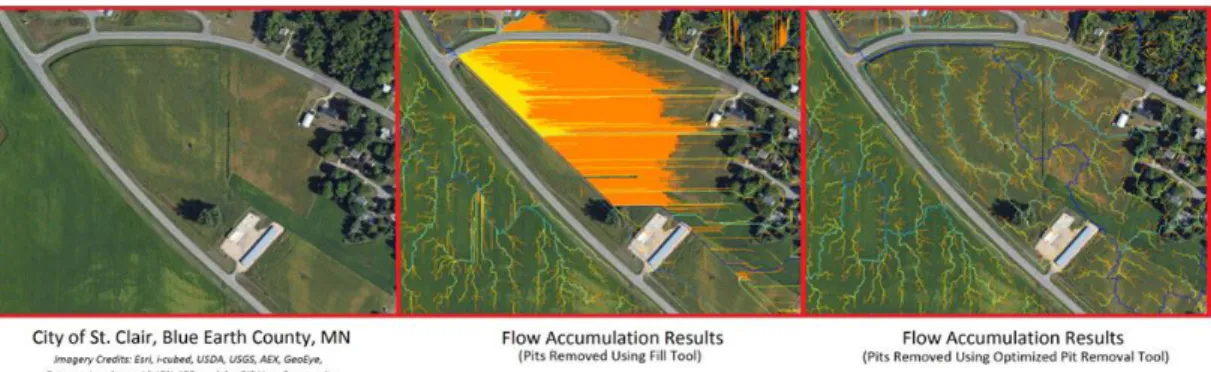
Figure 1. Comparison between Fill (left) and Optimized Pit Removal (right) tools
(Jackson, 2012) ... 7
Figure 2. Delineation of drainage lines in flat areas with Fill (middle) and Optimized Pit Removal tools (right) (Jackson, 2012) ... 7
Figure 3. Example of a cost surface (dark areas represent higher resistance) ... 10
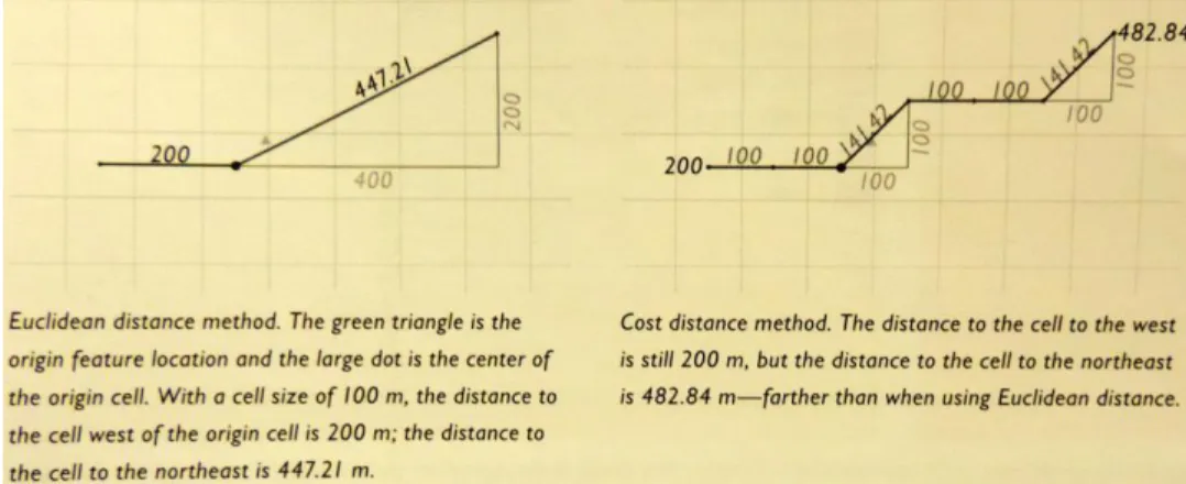
Figure 4. Comparison between Euclidean (left) and cell-to-cell (right) distances (Mitchell, 2012, p. 219) ... 11
Figure 5. Cost distance surface (left) and cost direction layer (right) (ESRI, 2015) ... 12
Figure 6. Cost direction layer. Direction coding (left) and directionality (right) (ESRI, 2015) ... 12
Figure 7. Example of an LCP between an origin and multiple destinations ... 13
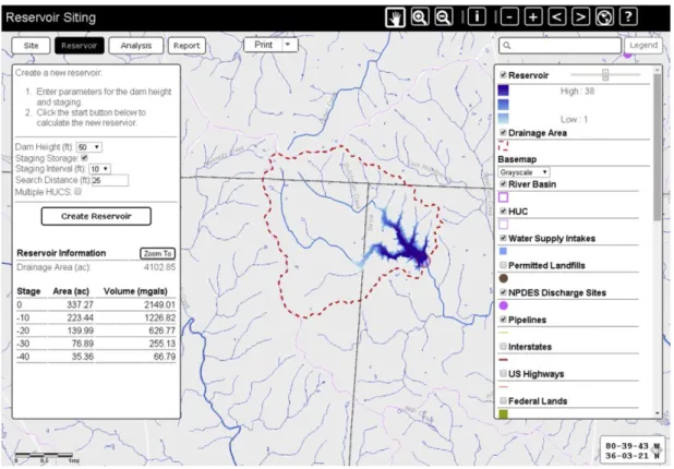
Figure 8. The NC-RES tool (Walsh et al., 2015) ... 16
Figure 9. Location of study area ... 18
Figure 10. Tiles downloaded of the SRTM at 1 arc second. ... 21
Figure 11. Land use/Land cover (LULC) map (Duarte et al., 2014) ... 22
Figure 12. Protected basins in Honduras (Cardona, 2010) ... 23
Figure 13. Flowchart of the methodology ... 25
Figure 14. Tiles merged of the study area ... 26
Figure 15. DEM of the study area ... 26
Figure 16. Data model for definition of hydrologic characteristics ... 27
Figure 17. Data model for finding the best path between the parcel location and water intakes/outlets ... 31
Figure 18. Cost path model for multiple destinations ... 32
Figure 19. Hosepipe path 1 (surface length 3,363 m) ... 36
Figure 20. Hosepipe path 2 (surface length 2,723 m) ... 37
Figure 21. Hydrologic characteristics for a small window of the study area ... 38
1.
INTRODUCTION
The Government of Honduras, the U.S. Agency for International Development (USAID) and the International Center for Tropical Agriculture (CIAT) are working together to try to establish a solution to the water shortage in Western Honduras. This area is affected by extreme climatic conditions and cyclical droughts related to the phenomenon of El Niño-Southern Oscillation (ENSO) (FAO & ACF, 2012). The study area of this project is located in Western Honduras and is part of the Centro American “dry corridor” (corredor seco) which is formed by some areas of Guatemala, Honduras, El Salvador and Nicaragua (FAO & ACF, 2012).
Whether the water demand of crops is supplied and the water availability is improved, farmers can get incomes based on the yield of each parcel. Therefore, farmers will be less vulnerable to extreme climatic conditions and agricultural loss. Information to support decision making on addressing water catchments is not currently available in the study area. Given this, a Geographic Information System (GIS)-based solution can be implemented as has been used through the world by researchers for identifying sites where farmers can obtain water as supply for crop irrigation (Al-Adamat, Diabat, & Shatnawi, 2010; El-Awar, Makke, Zurayk, & Mohtar, 2000; Shatnawi, 2006).
The present study provides the methodology implemented and results obtained in order to develop a GIS-based tool to address water captures in Western Honduras. This tool can be used by decision makers to geographically determine sites for water management and agricultural investments. It combines decision rules and surface features such as slope, vegetation and some protected basins. Based on these, two versions of the tool were developed. Both desktop and online versions were created by using software developed by Environmental Systems Research Institute, Inc. (ESRI1). The desktop version is a toolset which was implemented in ArcGIS for
Desktop2 as a toolbox. On the other hand, the online web application was developed by using ArcGIS Online3, Web AppBuilder for ArcGIS4 and two geoprocessing
services created through ArcGIS for Desktop and ArcGIS for Server5.
1.1 Problem Statement
As water is the main source for human welfare and agricultural production, its access, therefore, is among others, one of the most important constraints to successfully achieve the latter. This dependency on water in conjunction with conditions of extreme poverty it is the current scenario of the Western part of Honduras. It is clear so the need for identifying new or better sites for water catchments in the region. This thesis work provides a tool which is based on GIS and surface features to address water captures for small irrigation projects in the study area. This can be achieved by
1http://www.esri.com/
providing paths with the least costs of crossing the surface, through which it is possible to install hosepipes to take water from surrounding streams. Also, by guarantying that the intake points are not located in protected areas and above the parcel location.
1.2 Objectives
Main objective: To identify feasible water catchments for small irrigation projects in
Western Honduras based on GIS and surface features.
Specific objectives:
To identify geographically the paths with the least costs of crossing the surface for better targeting of water capture investments.
To create a GIS-based tool to identify water catchments in Western Honduras which is based on common decision rules and set of criterion layers.
To validate the ability to identify water catchments of the tool developed in this thesis based on verification of previous/current experiences of water capture projects in the study area.
1.3 Thesis Structure
2.
LITERATURE REVIEW
The present review provides a brief description of what a Digital Elevation Model (DEM) is, the main processes to achieve a hydrologically conditioned DEM, the basis of modeling an overland path and how the process to extract hydrologic characteristics from a DEM is accomplished. Also, some related works are presented.
2.1 Digital Elevation Model (DEM)
The topographic surface of any place over the world can be represented with a DEM. This is the acronym for Digital Elevation Model. Many definitions of this term exist. According to the GIS Dictionary of ESRI6, a DEM is “the representation of continuous elevation values over a topographic surface by a regular array of z-values, referenced to a common datum”. In a shorter way, the U.S. Geological Survey (1993) argues that a DEM “consists of a sampled array of elevations for a number of ground positions at regularly spaced intervals”. In accordance with the aforementioned definitions, it is possible to say that any raster (grid format) which represents the elevation of a portion of terrain can be considered as a DEM.
DEMs have been used worldwide for multiple kinds of applications such as hydrological modeling, flood modeling, orthorectification of aerial imagery, viewshed analyzes and many more (Hirt, Filmer, & Featherstone, 2010; W. Zhang & Montgomery, 1994). Among the wide variety of applications, in combination with GIS, these are fundamental to determine hydrologic parameters of watersheds such as catchment delimitation and its corresponding stream network (Choi, 2012; Li, 2014; Maune, 2007; H. Zhang, Huang, & Wang, 2013). Actually, they define how the water flows through the land surface (H. Zhang et al., 2013), which is essential for distributed water-based models (Colombo, Vogt, Soille, Paracchini, & de Jager, 2007; Li, 2014; H. Zhang et al., 2013).
W. Zhang and Montgomery (1994) mention two formats to store digital elevation data. On one hand is point elevation data, which in turn can be classified as a regular grid or Triangular Integrated Network (TIN) and; on the other hand, we have line contours. Both formats offer different advantages and disadvantages but as mentioned by W. Zhang and Montgomery (1994), grid format has been more widely used since availability of elevation data has increased with the need for environmental monitoring and management, land surface modeling, study of catchment dynamics and many more (Huang, 2003; Reuter, Nelson, & Jarvis, 2007; Wu, Li, & Huang, 2008; W. Zhang & Montgomery, 1994).
Among the most of the globally widespread DEMs at present are the Shuttle Radar Topography Mission (SRTM) and the Advanced Spaceborne Thermal Emission and Reflection Radiometer (ASTER) Global Digital Elevation Map (GDEM). As described in Farr et al. (2007), the SRTM flew in February 2000 and was a cooperation between the National Aeronautics and Space Administration (NASA), the National Geospatial-Intelligence Agency (NGA), and the German and Italian Space Agencies. In this mission, it was collected data of about 80% of the Earth’s land surface located between 60° north and 56° south latitude. In 2003, the SRTM data was released at 1 arc second of spatial resolution (approximately 30 m at the equator) for the United States and at 3 arc seconds (approximately 90 m at the equator) for the rest of the world (Jarvis, Reuter, Nelson, & Guevara, 2008). Years later, in 2014, it was globally released the SRTM data at 1 arc second7. The SRTM data can be downloaded from numerous websites but one of the most recognized is the USGS EarthExplorer which can be consulted at http://earthexplorer.usgs.gov/. On the other hand is the ASTER GDEM, and according to METI/NASA (2009) the data “was generated using stereo-pair images collected by the ASTER instrument onboard Terra”. GDEM V2 is the latest version and adds 260,000 additional stereo-pairs to the version 1 whose coverage spans from 83° north latitude to 83° south (approximately 90% of the Earth’s land surface). This data is freely available at 1 arc second of spatial resolution
at https://asterweb.jpl.nasa.gov/gdem.asp.
Despite the advantages and diverse uses of the aforementioned DEMs, some studies provide evidence that the SRTM presents better quality of topographic data in comparison with ASTER (e.g. Hirt et al., 2010; Nikolakopoulos, Kamaratakis, & Chrysoulakis, 2006; Rajabu, 2005; Wong, Tsuyuki, Ioki, & Phua, 2014).
2.1.1 Hydrologically Conditioned DEM (Hydro DEM)
For many water resource applications concerning to the simulation of water flow over the land surface (Soille, 2004), it is indispensable to extract stream networks and to delimitate drainage areas. Before carrying out these processes, it is necessary to hydrologically correct the DEM (Reuter et al., 2007; Ulmen, 2000). This terminology is used for a sink-free DEM (i.e. depressionless) whose flow direction follows the expected flow over the land surface (Djokic, 2011; Ulmen, 2000; Wu et al., 2008).
A sink is a pixel which impedes the continuous downslope flow of water. It is located at the lowest point of a depression (a bunch of pixels) which does not have an outlet. It is possible that sinks are real in the landscape, natural depressions like karst areas, but they can also be resulting artifacts of pre-processing operations such as resampling processes (Wu et al., 2008). In order to obtain a stream network with flow paths reaching their corresponding outlets as well as ensuring the proper delineation of basins, spurious sinks have to be removed in advance (Soille, 2004).
The software ArcGIS contains the Fill tool for sink removal of a DEM. This tool
works by filling each sink encountered in the DEM, to the height of the boundary cell with the lowest elevation of the contributing area of the sink (Jenson & Domingue, 1988; Wu et al., 2008). According to Jackson (2012), this tool could not be effective for hydrologically conditioning of DEMs due to the increment in the average elevation of the terrain and the creation of unnatural smooth areas. Instead of that, he proposes a new Optimized Pit Removal V1.5.1 tool8, which is an implementation of
the methodology described by Soille (2004). In Figure 1 both conceptual depictions are compared.
8 This tool is freely available at
Figure 1. Comparison between Fill (left) and Optimized Pit Removal (right) tools (Jackson, 2012)
The Optimized Pit Removal tool attempts to minimally affect the landscape by a combination of cut and fill, in order to eliminate sinks encountered in the DEM. In flat areas, where the definition of streams is erratic and it is infeasible to acquire vector data of known drainage lines, this tool enables the delineation of detailed flow paths (Figure 2).
Figure 2. Delineation of drainage lines in flat areas with Fill (middle) and Optimized Pit Removal tools (right)
(Jackson, 2012)
ArcGIS also contains the Topo to Raster tool that attempts to create a hydrologically
In any case, the most important aspect of this process is the flow pattern (Djokic, 2011). Knowledge obtained from field work and about the weather of the study area is very useful to hydrologically condition a DEM. Additionally, alternate sources of topography and hydrologic data will allow to better carry out this process. If supplemental data is not provided, this process can be iterative until the flow direction suits the assumptions made on the flow pattern (Djokic, 2011).
2.1.2 Extraction of Hydrologic Characteristics from a DEM
DEMs have been used worldwide for the extraction of hydrologic characteristics such as stream networks and drainage areas (Choi, 2012; Li, 2014). However, as mentioned in section 2.1.1, it is fundamental to hydrologically condition the DEM beforehand. Topographic attributes such as slope gradient and slope aspect are also possible to be extracted from a DEM (Jenson & Domingue, 1988; Wu et al., 2008).
Multiple studies have been carried out to automatically extract hydrologic characteristics from a DEM (Choi, 2012; Soille, 2004; H. Zhang et al., 2013). Although many applications exist to obtain theses DEM derivatives, most of them use the D8 algorithm (i.e. deterministic 8) to calculate the flow direction (Melles et al., 2011). This is a single flow direction algorithm developed by O’Callaghan and Mark (1984) which uses neighborhood information from the eight nearest cells to direct the flow from each cell in the grid. This direction is the direction from the analyzed cell to the steepest downslope neighbor (O’Callaghan & Mark, 1984; Soille, 2004). In Tarboton (1997), however, are discussed other algorithms that implement multiple flow directions by applying on each cell weights from its neighbors.
Stream networks and drainage areas are based on the calculation of the flow direction and the flow accumulation (Choi, 2012; Jenson & Domingue, 1988; Metz, Mitasova, & Harmon, 2011; Wu et al., 2008). In order to determine the stream network of a basin, a stream threshold value has to be subjectively defined by the user (Li, 2014; Melles et al., 2011; H. Zhang et al., 2013). A cell belongs to the stream network if its accumulated flow value exceeds this threshold (Jenson & Domingue, 1988; Soille, 2004). This latter indicates, in turn, the upstream contributing area draining to that cell (Soille, 2004; H. Zhang et al., 2013). Although this value should be mostly based on geomorphological and weather characteristics (Soille, 2004; H. Zhang et al., 2013), most of times is arbitrarily assigned (H. Zhang et al., 2013). The greater the threshold value, the less dense the stream network (Jenson & Domingue, 1988). This value is vital and influences the definition of the stream network and consequently of the drainage area. To define this latter, it is necessary to delineate the area that drains surface water to a specific point located downslope (Choi, 2012; Soille, 2004). The surface water converges to this point which is the exit of the basin also called outlet.
The aforementioned processes can be carried out by using GIS-based software such as SAGA GIS9, QGIS10, gvSIG11 or ArcGIS. This latter, as the GIS software chosen for
this thesis work, provides the “Hydrology” toolset which contains tools to create a stream network or delineate watersheds. ESRI (2011) also provides Arc Hydro, which is an ArcGIS-based system aimed to support applications related to water resources (Djokic, Ye, & Dartiguenave, 2011). It has two main components which are Arc Hydro Data Model and Arc Hydro Tools. By using Arc Hydro and following the workflows suggested by ESRI (2013), it is possible to perform analysis often related to the water resources area. Based on the SRTM DEM and using Arc Hydro tools, the stream network and catchment areas will be modeled for the study area of this thesis.
2.2 Overland Path Modeling
Modeling an overland path falls on the subject of Least-Cost Analysis (LCA). This latter is a distance analysis tool enabled by GIS technology that allows finding the Least-Cost Path (LCP) between two locations. By using LCP method, it is possible to
9http://www.saga-gis.org/
model movement across the surface while minimizing the cumulative cost along it (Melles et al., 2011; Mitchell, 2012; Rivera, 2014). This modeling is based on the idea that any movement across the surface implies a cost (Mitchell, 2012). Given this, the cost can be optimized in order to obtain the most cost-effective route between origin and destination. LCP is a raster-based method which relies on a resistance/friction surface (Theobald, 2005)—also known as cost surface as shown in Figure 3. This surface is a raster dataset commonly generated by making a weighted overlay of variables that influence the movement of the phenomenon to be modeled. The cost of each cell, in the cost surface raster, represents the cost of crossing it. This cost can be time, distance, money or any other variable defined by the modeler (Mitchell, 2012).
Figure 3. Example of a cost surface (dark areas represent higher resistance)
Many factors can influence the movement or its direction. For example, slope as being anisotropic (Herzog, 2013), can increase or decrease the real distance of the movement. In the case of water through a pipeline/hosepipe, the slope can speed up the movement while moving downhill or decelerate it in uphill direction (Mitchell, 2012). Other factors such as vegetation, lake, rivers, fences or roads play an important role as impedance surface factors (Mitchell, 2012; Rivera, 2014). Additionally, protected areas should be mostly avoided by LCP and they can also be included as a factor to derive the cost surface.
achieved by using a cost distance surface which reflects the cumulative distance from the pixel containing the origin to each of the other pixels (Mitchell, 2012).
Figure 4. Comparison between Euclidean (left) and cell-to-cell (right) distances (Mitchell, 2012, p. 219)
The steps to model an overland path can be encapsulated in three main phases as described by Rivera (2014): Preparation, analysis and output. These steps can be executed in ArcGIS which provides tools to achieve the modeling of an LCP.
Preparation
Firstly, any source layer has to be clipped by using the boundary of the study area. The source layers (e.g. slope, vegetation and protected areas) should be rasterized if they are in vector or another format. Then, a reclassification process has to be carried out in order to classify the rasterized source layers into a ratio scale12 (Mitchell, 2012). Categorical and continuous layers, such as vegetation and slope, need to be converted in values into the defined scale. The higher the cost value, the more difficult to cross over. Therefore, steeper slopes can be represented by higher values and flat areas by lower values. It works similarly for vegetation. Zones with forests or riparian covers are represented by higher values because it is more difficult to cross these areas than, for example, grasslands. The movement over some areas, such as protected areas, has to be restricted and, therefore, the highest value into the scale should be assigned.
12As defined by Stevens (1946), one characteristic of a ratio scale is that it entails an absolute zero as is the case of
Analysis
This is the main phase of the entire process. It is composed of the creation of both the cost surface and the cost distance surface; and the modeling of the best path (LCP). As mentioned before, LCP is based on a resistance/friction surface which is in turn based on impedance factors. These factors are criterion layers defined for the model. For instance, in the modeling of a wildfire, factors such as vegetation and slope influence the ease/difficulty of the movement (Mitchell, 2012). The combination of them allows creating an overall surface (e.g. Figure 3). The cost surface is the result of a weighted overlay process taking as inputs these criterion layers. For each of these layers, a weight is assigned which represents its importance into the model. The sum of the weights has to be equal to 100%. If for example, vegetation, slope and protected areas are used as inputs for the model, then weights of 40%, 40% and 20% can be respectively assigned.
The cost surface and the location of the origin are the inputs for the cost distance model. In this step, the cost distance surface (Figure 5) and the cost direction layer (Figure 6) are created. While the former provides the cumulative cost of travel outward from the origin, the latter defines the direction of travel from each cell to the next neighboring cell along the LCP (Mitchell, 2012). The values in this layer are ranged from 0 to 8, where 0 is the value assigned to the cell that represents the origin location (Figure 6).
Figure 5. Cost distance surface (left) and cost direction layer (right) (ESRI, 2015)
Finally, after the required inputs for the cost path model are created, then it is possible to find the best path (LCP), which is a point-to-point path between the origin and the provided destination (Mitchell, 2012). In the case of a pipeline, for example, the origin and destination are connected by the most cost-effective route. The LCP depends so, on the criterion layers used as impedance surface factors, the defined scale, the classification of the layers and the weights assigned to them.
Results
The resulting LCP will be only one cell wide (Theobald, 2005), which can be later converted to a vector format if desired. For the last aforementioned case, only one destination is provided. However, it is possible to model different paths from the same origin to multiple destinations as shown in Figure 7 (Mitchell, 2012). This is the case when more than one possible destination is provided in order to compare among the different resulting LCPs. Through the demonstration of concept of this thesis, multiple catchment points from streams will be evaluated for a provided origin, which in this particular case is the farm location.
Figure 7. Example of an LCP between an origin and multiple destinations
In particular, Herzog (2014) provides a revision of 15 recent archeological studies (dated between 2012-2013) where LCA has been used to calculate site catchments, LCPs or accessibility. In another case, Melles et al. (2011) used an LCP approach to the delineation of streams using lakes as patches and a DEM as a cost surface.
In a recent paper, Rivera (2014) presents a novel approach of using LCP. In this study, LCP is used to predict a possible route that an illegal immigrant would take from a location surrounding the international border between U.S. and Mexico, and a set location inside the U.S. territory. Rivera (2014) also mentions in his study, the possibility of using LCP for recreational use such as the development of a hiking route in order to save energy and conserve time and distance.
Other applications such as the installation of transmission lines or the design of a canal are also possible to be carried out by using the LCP model. Many more GIS applications could be mentioned. The diverse and multiple uses of this approach demonstrate its potential. For this thesis work, the LCP approach will be used in combination with decision rules and surface features. The latter will be used as criterion layers which determine the impedance surface factors of the model.
2.3 Related Work
have also evaluated other solutions such as transport water by trucking, shipping or open channels, though.
In other areas of the world such as Northern Jordan, a GIS-based water harvesting solution has been implemented to identify ponds in order to collect water for domestic, agricultural and livestock usages (Al-Adamat et al., 2010). As Jordan is a water-shortage country, many water harvesting projects have been implemented for centuries (Al-Adamat et al., 2010). Al-Adamat et al. (2010) propose to use GIS in combination with Weighted Linear Combination13 and Boolean techniques for the selection of suitable areas for water harvesting ponds in arid or semi-arid regions. This selection is based on socio-economic and physical characteristics of the study area; in the case of Northern Jordan were rainfall, slope, distance to Wadis, soils, and distances to urban centers and roads. The results of this study showed that 25% of the study area had potential to implement water harvesting ponds.
Water harvesting can also provide irrigation water for rainfed agriculture. Mwenge Kahinda et al. (2007) analyze the functions of water harvesting on agrological and hydrological basis as well as its impacts on crop yield. These analyzes were done in six districts of the semi-arid Zimbabwe. According to Mwenge Kahinda et al. (2007), supplemental irrigation provided by water harvesting technologies reduces the risks of crops to fail; converting them to more stable high productive irrigated crops. In Latin America, Pulver et al. (2012) established 12 reservoirs in Nicaragua and four in Mexico as a solution to provide surplus irrigation water for rainfed crops. This project focused on small crops with relatively low requirement of irrigation water. Rice and some irrigated crops as well as cattle, fish and dairy were taken into consideration. They introduced the concept of water harvesting in those areas and promoted its use by capturing and storing rainwater which can be used later as irrigation water. The implementation carried out in Pulver et al. (2012), resulted in increasing of crop productivity and farmer incomes.
Not going too far, in North Carolina, a novel tool for siting potential reservoirs was developed by Walsh, Page, McKnight, Yao and Morrissey (2015). The North Carolina
Reservoir Siting Tool (“NC-RES”, see Figure 8) is a GIS tool based on the web which allows non-specialist users to assess possible sites for reservoirs. This tool has been recently developed as an attempt to provide water supplies for the alarming low levels of water in drought periods. It is based on terrain data derived from North Carolina's LiDAR14. In addition, geospatial layers are used to assess the possible impacts of creating a reservoir in a desired location.
Figure 8. The NC-RES tool (Walsh et al., 2015)
NC-RES tool also allows users to perform spatial analysis such as reservoir inundation and drainage areas based on LiDAR derivatives. For the development of this tool, they used ArcGIS Server, ESRI map services and three geoprocessing services. ESRI JavaScript API was used to develop the interface of the tool.
All the aforementioned works were examined in this chapter because they have implemented approaches related in one way or another to the main objective of this thesis. In any case, these approaches will be taken into consideration for the implementation of the solution proposed in this thesis work for the current problem of water scarcity in the Western part of Honduras. It is important to mention that none of
3.
DESCRIPTION OF THE STUDY AREA
In this chapter are described the most important aspects of the study area related to this research.
3.1 Location
The study area is located in the Western part of Honduras in Central America and approximately covers the portion of the dry corridor that lies in the country (Figure 9). This area is surrounded by Guatemala in the West, El Salvador in the South, Nicaragua in the South East, the interior of the country in the East, and the Caribbean Sea in the North. The area compromises about 52,503 Km2 and spans from 15.900°N to 12.982°N latitude and from 89.353°W to 86.053°W longitude. It completely covers the departments of Choluteca, Comayagua, Copán, Cortés, Francisco Morazán, Intibucá, La Paz, Lempira, Ocotepeque, Santa Bárbara and Valle, and partially El Paraíso and Yoro.
3.2 Topography
The region is characterized by slopes ranging from 0° (coastal zones) to 74° (steep hills). The North and South of this area are lowlands while the interior is mountainous. The elevation ranges from 0 to 2,851 m.a.s.l. The study area contains mountains with the highest peaks of the entire Honduras. The Honduras’ mountains are merged to Guatemala’s mountains in the West and to Nicaragua’s mountains in the South East.
3.3 Climate
For the period 1992-2011, Honduras was one of the most vulnerable countries in the world due to extreme weather events (Gourdji, Craig, Shirley, & Ponce de Leon Barido, 2014; UNDP, 2011). As mentioned in chapter 1, the study area is affected by cyclical droughts related to ENSO (FAO & ACF, 2012). The area is characterized by a rainy season from May to November, leaving the rest of year as the dry season. The precipitation has a bimodal behavior that is interrupted by a dry period from mid-July to mid-August; which is called “canícula”. The rainy periods before and after “canícula” are called “primera” and “postrera” respectively (FAO & ACF, 2012). These latter ones define the two agricultural seasons in the area. The annual precipitation ranges from 800 mm up to 2,000 mm while the mean temperature varies from 6°C to 30°C (FAO & ACF, 2012).
3.4 Agriculture
In general, the agriculture in the study area is carried out in hillside lands by small-scale farmers who mostly plant corn during the Primera and beans during the Postrera. In some cases, a combination of both is also implemented. These crops are used primarily for their subsistence needs. In areas with steep slopes, they also plant coffee. As these crops are cultivated in hillside lands, are vulnerable to soil erosion and degradation, and consequently to a decrease in productivity (Paniagua, 1999; Wollni & Andersson, 2014).
for food production. Irregular precipitation, droughts as well as a lack of irrigation systems, entail that small-scale farmers can only produce two crops in a year.
3.5 Socioecomical Aspects
4.
RESOURCES USED
This chapter provides a description of the datasets, software, hardware and tools used in this thesis work.
4.1 Description of Data Used
The datasets used for the purpose of this research come from either public sources or courtesy of some institutions.
4.1.1 Digital Elevation Model (DEM)
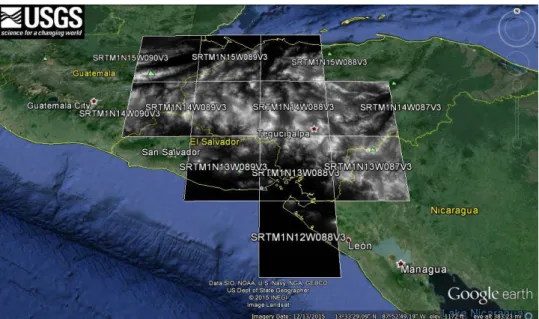
The SRTM DEM at 1 arc second of spatial resolution was used as elevation surface. The product “SRTM 1 Arc-Second Global” was downloaded from the USGS EarthExplorer web portal15 which offers worldwide coverage of void filled data. In Figure 10, it is possible to see the tiles downloaded for this DEM. Each square represents a 1 by 1 degree tile. 11 tiles were downloaded in GeoTIFF format which cover the total extension of the study area.
Figure 10. Tiles downloaded of the SRTM at 1 arc second.
4.1.2 Land Use/Land Cover
In this study it was used the Land use/Land cover (LULC) map which was elaborated at a minimum scale of 1:25,000 with Corine Land Cover classification for whole Honduras (Figure 11). It was generated from RapidEye imagery of 2012 and 2013 at 5 m of spatial resolution (Duarte et al., 2014). This dataset was provided in ESRI Shapefile format as a courtesy of the National Institute for Conservation and Forest Development, Protected Areas, and Wildlife (ICF).
Figure 11. Land use/Land cover (LULC) map (Duarte et al., 2014)
This map consists of 26 categories, eight (8) of which are forests and 16 non-forests. These categories can be clustered in five macro-categories: Forests (48%), agriculture and livestock (30%), other categories (18%), agroforest areas (2%) and water bodies (2%) (Duarte et al., 2014). The percentages represent the area of the Honduran territory (112,492 Km2) covered by each macro-category.
4.1.3 Protected Basins
Figure 12. Protected basins in Honduras (Cardona, 2010)
4.1.4 Validation Data
Some track points of current hosepipe paths as well as farm locations and their respective water intake points were provided by USAID. These datasets were taken with GPS in the field in collaboration with technicians of Fintrac Inc. These datasets were compared with the results provided by the tool implemented in this thesis as will be discussed later in sections 5.6 and 6.3.
4.2 Description of Software and Hardware Used
The software and hardware used for this research can be divided into two stages:
Development
The work was carried out using the GIS software ArcGIS 10.2.2 for Desktop in combination with Python 2.7, ArcPy and GPSBabel16. Complete features and specifications of the computer used are detailed in Table 1.
Table 1. Computer specifications
Operating System Windows 10 Home Single Language
Processor Intel(R) Core(TM) i7-3630QM 2.4 GHz
Number of processors 4
RAM 8 GB
Hard Drive 1 TB
Implementation
ArcGIS 10.2.2 for Desktop allowed the creation of two geoprocessing services which are used by the online web application. The latter was created by using Web AppBuilder for ArcGIS and stored on an organizational account of ArcGIS Online. ArcGIS 10.1 for Server houses the two geoprocessing services and is hosted on a server with the following specifications:
Table 2. Server specifications
Operating System Windows Server 2008 R2 Standard
Processor Intel(R) Xeon(R) E5450 3.00 GHz
Number of processors 8
RAM 32 GB
Hard Drive 10 TB
5.
METHODOLOGY
This chapter provides the methodological steps carried out to achieve the objectives of this thesis work. In Figure 13 is shown a flowchart of the methodology which provides an overall idea of the major steps, datasets and results of this thesis.
Figure 13. Flowchart of the methodology
It is very important to highlight that all the spatial information used in this work was projected to the spatial reference system “WGS84 UTM Zone 16 N” with datum WGS 1984. This process was carried out to avoid mismatches among the different layers used. Furthermore, it is indispensable to work with projected information for processes involving calculations such as linear distances, areas and slopes.
5.1 Pre-processing of the DEM
Figure 14. Tiles merged of the study area
The dataset in Figure 14 was then clipped with the boundary of the study area in order to obtain the raw DEM. This DEM is shown in the following figure:
After the dataset was clipped, it was possible to obtain the raw DEM of the study area with the corresponding range of elevations which goes from sea level till 2,851 m.a.s.l. It was not necessary to implement any void-filling algorithm or interpolation as the product downloaded “SRTM 1 Arc-Second Global” provides void filled data.
5.2 Definition of Hydrologic Characteristics
In order to obtain a hydrologically conditioned DEM (hydro DEM) for generating the streams and watershed delineations of the entire study area; the data model in Figure 16 was developed in ArcGIS for Desktop by using its application Model Builder. This data model was made based on Arc Hydro tools (ESRI, 2011) and following the workflows suggested by ESRI (2013). In addition, the Fill sinks process was implemented using the Optimized Pit Removal V1.5.1 tool developed by Jackson (2012).
Figure 16. Data model for definition of hydrologic characteristics
The input parameters for the data model in Figure 16 (blue ovals on the left) are the raw DEM of the study area (Figure 15), the workspace path and the threshold value for the definition of the stream network. As mentioned in Soille (2004) and H. Zhang et al. (2013), this latter should be defined based on geomorphological and weather characteristics, but most of the time is arbitrarily defined (H. Zhang et al., 2013). Given this, multiple iterations were carried out until this threshold value was finally set as 500. Therefore, any pixel with a flow accumulation value greater or equal to
Process Input
this threshold is part of the stream network. This value ensures a very well detailed stream network for the study area.
In general, the model removes all the local depressions (sinks) in order to generate continuous flows. Then it calculates the flow direction and flow accumulation based on the sink-free DEM. Some intermediate layers are later created. Finally, it defines all the outlets (drainage points), streams (drainage lines) and watersheds (catchment areas) of the study area. One possible step of creating a hydro DEM is to enforce drainages with stream features. It is possible to do so by rasterizing provided stream features and burning them into the DEM. The resulting surface will have deep channels that work well for routing flow and follow the real patterns. In this case, however, it was not possible to obtain supplemental data of streams for the drainage enforcement process. Therefore, the stream network was generated based on the sink-free DEM.
5.3 Least-Cost Path (LCP)
Before starting the implementation of the LCP method, it is necessary to condition the criterion layers used as impedance surface factors. For the specific case study of this thesis work, the criterion layers used were vegetation (LULC), slope and protected basins. The two first determine the difficulty of the movement whereas the latter mostly restricts the path over its areas. The objective of this process is to determine the best path from the farm location to an intake point (outlet) located in a surrounding stream. Over this path, then it is possible to install a hosepipe to capture water from the stream.
method “Natural Breaks (Jenks)” described in Jenks and Caspall (1971). The slope intervals defined in ArcGIS for Desktop with their corresponding cost values and areas are shown in Table 3.
Table 3. Cost values assigned to slope intervals using the classification method “Natural Breaks (Jenks)”
Interval Lower Limit (%) Upper Limit (%) Cost Value Area (Km2)
1 0.00 4.64 1 9,719
2 4.64 9.57 2 8,305
3 9.57 14.21 3 8,747
4 14.21 18.56 4 8,200
5 18.56 22.62 5 6,526
6 22.62 26.68 6 4,844
7 26.68 31.03 7 3,227
8 31.03 35.96 8 1,848
9 35.96 42.91 9 874
10 42.91 73.94 10 212
52,503
Table 4. Cost values assigned to LULC categories
LULC Spanish LULC English Cost Value Area (Km2)
Pastos y/o Cultivos Pastures and/or crops 1 17,079
Suelos Desnudos Continentales Inland bare soils 1 203
Vegetación Secundaria Seca Dry secondary vegetation 2 4,984
Vegetación Secundaria Húmeda Moist secondary vegetation 3 3,534
Árboles Dispersos Scattered trees 4 1,008
Café Coffee 4 2,334
Pino Ralo Sparse pine 5 3,703
Agricultura Tecnificada Technified agriculture 6 866
Palma Africana African oil palm 7 255
Bosque Mixto Mixed forest 8 1,863
Pino Denso Dense pine 8 7,534
Bosque Latifoliado Seco Broad-leaved dry forest 9 4,175
Bosque Latifoliado Húmedo Broad-leaved moist forest 10 3,210
Zonas Urbanizadas Discontinuas Discontinuous urban fabric 10 301
Áreas Húmedas Continentales Inland wetlands RESTRICTED 151
Arenales de Playa Beaches, dunes, sands RESTRICTED 2
Camaroneras y Salineras Shrimp farms and salt evaporation ponds RESTRICTED 177
Cuerpo de Agua Artificial Artificial water bodies RESTRICTED 87
Lagos y Lagunas Naturales Natural lakes and lagoons RESTRICTED 91
Mangle Alto Tall mangrove RESTRICTED 177
Mangle Bajo Low-height mangrove RESTRICTED 160
Otros Cuerpos de Agua Other water bodies RESTRICTED 238
Zonas Urbanizadas Continuas Continuous urban fabric RESTRICTED 373
52,503
The third layer used as impedance surface factor was the layer of protected basins. They compromise about 2,198 Km2 of the study area and were declared protected areas because they provide drinking water mainly to rural population (Cardona, 2010). In this specific case, a cost value of 10 was assigned to all of them. This cost value mostly restricts the installation of hosepipes over those areas but does not make it impossible. Indeed, it allows the model to avoid at most it is possible the path over such areas but in the extreme case where there is not a path with a less cost, the LCP method will provide a path traversing those areas.
into the defined scale. In addition, the farm location (origin) and the intake points (destinations) are also used as main inputs.
Figure 17. Data model for finding the best path between the parcel location and water intakes/outlets
The development of the data model in Figure 17 is based on the idea that any movement across the surface implies a cost (Mitchell, 2012). This cost can be optimized in order to get the least-cost path (LCP) of traveling from the origin to the destination(s). Therefore, it is necessary to have a cost surface which determines the ease/difficulty of traversing it. This cost surface was created by making a weighted overlay of the three impedance surface factors used for the study area. These factors were LULC, slope and protected areas. For each of these factors, a weight was assigned which represents its importance into the model. Since the sum of all the weights has to be equal to 100%, we assigned a weight of 40% for both LULC and slope, and of 20% for protected areas.
Firstly, the model creates the resistance/friction surface (cost surface) based on the three impedance surface factors. This is the part of the model that can be considered static as the cost surface is created only once. This surface can be changed if desired, but in our case, it was calculated based on the aforementioned cost values and weights. The middle and right parts of the model depend on both origin and destination(s), so in each modeling the cost distance and cost path processes have to be run. In order to establish an analysis area, it is created a buffer area of the merge of
Process Input
Output
40%
20%
both the origin and the destination(s). Then, this area is set as the analysis extent of the cost distance process.
The drainage points/outlets obtained in the extraction of hydrologic characteristics (section 5.2), were used as potential locations where farmers could take water from streams. These captures allow farmers to use supplemental irrigation water for rainfed crops due to most of them practice rainfed subsistence agriculture in the Western part of Honduras. In Figure 17, these outlets—also called as intake points—are provided as destinations for the data model.
By using the data model shown in Figure 17, it is possible to model different paths from the same origin to multiple destinations. Therefore, multiple intake points from streams are evaluated for a provided origin, which in this particular case is the farm location. The multiple calculations are carried out in the cost path model by iterating among the different destinations as shown in Figure 18. This latter is a submodel of the model in Figure 17 and allows modeling more than one LCP from the same origin. Furthermore, it adds valuable surface information such as maximum, mean and minimum slopes, and surface distance. This surface information is calculated based on the raw DEM. The surface distance is a very important characteristic of the LCP because determines how long the hosepipe will be. This implies the length of the path and, therefore, the money that farmers need to invest in buying the hosepipe. Another important aspect is the slope because provides an overall description of the topography over which the hosepipe will be installed.
Figure 18. Cost path model for multiple destinations
points (destinations). The automation processes for both desktop and online versions are explained in the following sections.
5.4 Requirement Analysis
In order to develop a tool to identify feasible water catchments for small irrigation projects in Western Honduras, we first had an approach with population of the study area. This approach was carried out through a meeting with around 20 participants in which were integrated some farmers and people from different institutions such as USAID, Fintrac and CIAT. While the former are the target population of this study, the latter are the possible users of the tool. Furthermore, we also had a field trip in the department of Intibucá to understand and realize the serious conditions of both poverty and water scarcity.
The first approach was very important and fundamental for the development of this thesis work. On one hand, because we could hear and understand the current problems in the study area by means of informal interviews with stakeholders. On the other hand, they explained us through in-field observations, how the current water catchments work and what the procedures to install them are. The most important remarks we received from farmers as well as from technicians can be summarized in the following bullets:
Farmers take water from streams through hosepipes/pipelines trying to avoid the installation of pumps in between of the water intake and the farm location. This is done in order to reduce investments. As a solution, they mostly take water from upper areas using gravity to impulse it until the farm location.
It is very important the length of the path, so they look for possible water intakes in streams not so far from their farms.
It is restricted to install water intakes in the basins declared as protected areas.
Based on these remarks, we established the decision rules to find feasible water intakes for a farm. The solutions proposed to solve/deal them were:
The tool has to look for water intakes located above the farm location. Therefore, it is necessary to obtain the elevations of both farm location and each water intake and then to filter the water intakes that are at least 10m above the farm location.
The tool has to allow the user to search water intakes within a linear radius from the farm location.
Any water intake located within the protected basins has to be discarded.
It is necessary to allow the user to convert from GDB and GPX files to a format established as input for the tool. Also, the results should be exported to a file format readable by handheld GPS devices (i.e. KML).
Water intakes that go through the first three of the previous conditions are considered potential sites for a farm. If more than five sites are found by the tool, they are restricted to only five. These sites are provided in ascending order based on their surface distances to the farm location. In any case, this amount of potential sites is sufficient to find the most feasible one for the farm. The final sites, where is possible to take water from streams, are provided as destinations to the model in Figure 17.
5.5 Development of the Tool
The remarks provided by the stakeholders allowed us to develop the tools presented in this thesis. These tools were developed to be used by either technicians or decision makers who can address the process and help farmers to solve their problems related to water supply. In the following sections are explained the two versions developed in this thesis work.
5.5.1 Desktop Version
and output parameters and contain their corresponding metadata. The tools stored on this toolset were the following:
1. GDB To Shapefile / GPX To Shapefile 2. Best Paths
3. Generate Watersheds 4. Results To KML
The numbers in the names of the tools indicate the possible sequence to be followed in order to have a successful and complete run. This depends, of course, on what the user wants to do. The two tools, whose names are preceded by the number “1”, can be both firstly executed based on the need of converting from either GDB or GPX format to Shapefile. The essential tools of this toolset are “2. Best Paths” and “3. Generate Watersheds”. While the former determines the best paths (LCPs) from a farm location to potential water intakes, the latter defines the drainage areas of these sites. Most of these tools need basic information to carry out their processes. In consequence, this information was stored on a geodatabase which consists of the raw DEM, the hydrologic characteristics (i.e. outlets, stream network and catchment areas), the protected basins and the cost surface.
This desktop version was developed to be mainly used in office but it is also possible to use it in the field with a laptop. It is necessary to have ArcGIS for Desktop and Python installed on the computer. The latter, however, is automatically installed with ArcGIS for Desktop. In addition, the software GPSBabel is also required since it is used by the tool “1. GDB To Shapefile” to convert from GDB (MapSource) to GPX (GPS eXchange) format.
5.5.2 Online Version
with ArcGIS for Server installed. It is important to mention that in the creation of the geoprocessing services with ArcGIS for Desktop and ArcGIS for Server, it was necessary to make some relevant changes in the toolbox, input formats and scripts in order to avoid future problems which could take long time to solve them.
By using Web AppBuilder for ArcGIS, the online web application was finally built and stored on an organizational account of ArcGIS Online. The online web application uses the two geoprocessing services as well as ready-to-use widgets. As a result, the final version of the online web application eliminates the user’s dependency of using a computer to run the main tools, because it can be run on a mobile device. On the other hand, the online web application has the drawback of requiring Internet access.
5.6 Validation of the Tool
The information supplied by USAID consisted of track points of two current hosepipe paths with their respective water intakes and farm locations. They were captured in 2015 in the municipality of Yamaranguila, department of Intibucá. The two following figures show in perspective the paths of the two current hosepipes.
Figure 20. Hosepipe path 2 (surface length 2,723 m)
These datasets were converted to Shapefile format and compared with the results provided by the tools “2. Best Paths” and “3. Generate Watersheds”. For running the former, it was set a search radius of 10 Km from the farm location. Additionally, the elevation difference between the potential water intakes and the farm location was set as 10 m. The latter is the minimum elevation difference allowed by the application in order to bring water by using gravity. In this process, we calculated the surface distances, the costs of both current and modeled paths and determine the drainage area of each site.
6.
RESULTS AND DISCUSSION
The results achieved through the demonstration of concept of this thesis, their respective analyzes as well as some discussions are presented in this chapter.
6.1 Hydrologic Characteristics
The hydrologic characteristics obtained from the hydro DEM were the outlets (drainage points), streams (drainage lines) and watersheds (catchment areas). As a result, 59,172 watersheds were delimited and consequently the same amount of outlets was defined. Since all of these results were defined at a very detailed scale, it is impossible to appreciate their features at a general view, therefore, some of them are shown in Figure 21 for a small window of the study area.
Figure 21. Hydrologic characteristics for a small window of the study area
spatial resolution enables the definition of more accurate hydrologic characteristics but at the same time it is also necessary more processing and storage capacity. Local elevation datasets—such as contours or elevation points—and alternate sources of hydrologic data could help to improve the detail and accuracy of the results. Unfortunately, we could not obtain supplemental information to better carry out this process. Another important factor is the threshold value for the delimitation of the stream network and consequently of the watersheds. As discussed before, this is considered a vital factor and should be based on geomorphological and weather characteristics. Nevertheless, in our case, it was defined after multiple iterations changing its value. Anyway, for the purpose of this thesis work, the detail worked was good enough to accomplish the successful results obtained.
It is important to mention the usage of each of these results. Therefore, the drainage points/outlets were used as potential locations where farmers could take water from streams. They are also called as intake points and the resulting ones that go through the decision rules explained before (section 5.4), are provided as destinations for the data model in Figure 17. Subsequently, the streams provide an idea of how water flows in the channels of the study area. Based on the streams, the outlets and watersheds were defined. Finally, the latter were used to give an idea of the areas that drain surface water to potential water intake points. In consequence, the three hydrologic characteristics are used by both the desktop and the online versions of the implemented tools.
6.2 Tool to address water captures in Western Honduras
Figure 22. Cost values of slope (a), LULC (b), protected basins (c) and cost surface (d)
The final cost surface contains voids because of the LULC layer. The latter consisted of categories which were assigned as “NoData” when rasterizing it based on its cost values. These are the categories classified as “RESTRICTED” in Table 4. The cost values were assigned based on the idea that both slope and LULC determine the difficulty of the movement whereas the protected areas mostly restrict the path over their areas. Therefore, these cost values are meaningful and realistic attempts to represent the ease/difficulty of traversing the surface to install a hosepipe. Anyway, it would have been a great idea to contrast these cost values with personal opinions of farmers, and thus define them based on the real effort that they make to traverse any of the LULC categories.
taken as two times more important than the protected areas. However, for other applications, a different set of weights can be applied based on different criteria. Even it is possible to integrate different impedance surface factors, and then design scenarios to be contrasted in order to define the final cost surface that better represent the phenomenon to be studied. In the latter case, it would be necessary then to validate the correctness of the results with the real conditions of the movement over such a surface.
Cost values and weights play the most important roles when defining the LCP. As it is hard to quantify these values in order to represent the reality, it is necessary to contrast the results with knowledge from either experts or people who know about the study area. Even in some cases, including additional layers in the modeling provide more realistic conditions of the area. Therefore, it is notable that LCP depends on factors such as the criterion layers used as impedance surface factors, which in turn depend on the scale at which they were created, the classification of the layers and the weights assigned to them.
The cost surface, the hydrologic characteristics, the raw DEM and the protected areas were stored on a geodatabase to be used by the tools packaged as a toolset in ArcGIS for Desktop (Figure 23). Two of them (tools enclosed by yellow rectangles in Figure 23) were published as geoprocessing services which are in turn used by the online web application.
Figure 23. Tools packaged as a toolbox in ArcGIS for Desktop. In yellow rectangles, the tools published as geoprocessing services.
Table 5. Overview of tools developed
Tool Name Description
Version Toolbox ArcGIS
Online Web App.
1. GDB To Shapefile
It converts waypoints stored in a GDB file (MapSource format) to Shapefile format (.shp). To run it, it is necessary to have installed the GPSBabel software. It also extracts the elevation from the DEM for each of the waypoints.
X
1. GPX To Shapefile
It converts waypoints stored in a GPX file (GPS eXchange format) to Shapefile format (.shp). It also extracts the elevation from the DEM for each of the waypoints.
X
2. Best Paths
It determines which the best paths from the outlets to the parcel location in a specified search radius are. All the processes are based on the Cost Surface previously calculated by running a weighted overlay using as inputs the vegetation, slope and protected areas.
X X
3. Generate Watersheds It creates polygons of drainage areas given the final outlets which should have been created by executing
the tool "2. Best Paths". X X
4. Results To KML
This tool converts the resulting Feature Dataset obtained by running the tools "2. Best Paths" and "3. Generate Watersheds", to KML. This file is compressed using ZIP compression, has a .kmz extension.
X
These tools enable the user to carry out a complete process, from converting to Shapefile the farm coordinates taken with a handled GPS in the field, until obtaining in KML format the potential water intakes for that farm, the best paths to reach them and the areas that drain to them. If the user decides to use the online web application, he/she does not need any computer, just a mobile device with Internet and consequently he/she is able to run the main tools but analyzing in real time the results provided by it. Besides, it permits to export the results as a CSV file, Feature Collection or GeoJSON. The online web application can be seen by clicking on the following link:
http://csi.maps.arcgis.com/apps/webappviewer/index.html?id=713cf0cf71c44bdda3d1
213768ffb1be.
Figure 24. Online web application
When opening it, the user sees an information window with explanations about how to run the two geoprocessing services included into the application. In addition, it allows the user to change the basemap and print the map with the current view. Also, it is possible to use the ESRI World Geocoder to search for a place in the world. Moreover, the legend and the layer list are ready to use on the right side. By using the latter, it is possible to see the attribute tables of the resulting layers and, therefore, make filters and sort any field of a layer. Figure 25 shows how the application looks like after a complete run for a specified position of a farm (parcel).
6.3 Validation of the Tool
For each of the current hosepipe paths used to validate the tool developed in this thesis work, we modeled five other different potential paths that connect the farm to sites different—close in some cases—to the current water intakes. The sites provided by the tool are a subset of the outlets obtained in the definition of hydrologic characteristic. These are located exactly on the conjunction of streams as an attempt to find sites with enough water to supply the subsistence needs of farmers. On the other hand, the paths modeled by the tool are least-cost paths (LCPs), i.e., paths optimized to obtain the most cost-effective routes between the farm and feasible water intakes. Figure 26 provides an overall outlook of the current paths and the results obtained by the tool.
Figure 26. Comparison between the current hosepipe paths and the paths modeled by the tool