Estimating the optimum size of a tidal array at a multi-inlet system considering environmental and performance constraints

Estimating the optimum size of a tidal array at a

multi-inlet system considering environmental and

performance constraints

Corresponding Author: Eduardo González-Gorbeña1 E-mail: [email protected]

Telf.: +351 915113242 André Pacheco1

E-mail: [email protected]

Theocharis A. Plomaritis1,2

E-mail: [email protected]@uca.es

Óscar Ferreira1

E-mail: [email protected]

Cláudia Sequeira1

E-mail: [email protected]

1_{Centre for Marine and Environmental Research (CIMA), Universidade do Algarve (UAlg),} Edifício 7, Campus de Gambelas Faro, 8005-139, Portugal.

2_{Faculty of Marine and Environmental Science, Department of Earth Science, Universidad de} Cádiz, Campus Río San Pedro (CASEM), Puerto Real 11510, Cádiz, Spain.

Doi: https://doi.org/10.1016/j.apenergy.2018.09.204

Abstract

This paper investigates the optimum tidal energy converter array density at a tidal inlet by applying surrogate-based optimisation. The SBO procedure comprises problem formulation, design of experiments, numerical simulations, surrogate model construction and constrained optimisation. This study presents an example for the Faro-Olhão Inlet in the Ria Formosa (Portugal), a potential site for tidal in-stream energy extraction. A 35 kW EvopodTM _{floating tidal} energy converter from Oceanflow Energy Ltd. has been used for array size calculations considering two design variables: 1) number of array rows, and 2) number of tidal energy converter per row. Arrays up to 13 rows with 6 to 11 tidal energy converters each are studied to assess their impacts on array performance, inlets discharges and bathymetry changes. The analysis identified the positive/negative feedbacks between the two design variables in real case complex flow fields under variable bathymetry and channel morphology. The non-uniformity of tidal currents along the array region causes the variability of the resource in each row, as well as makes it difficult to predict the resultant array configuration interactions. Four different multi-objective optimisation models are formulated subject to a set of performance and environmental constraints.

Results from the optimisation models imply that the largest array size that meets the environmental constraints is made of 5 rows with 6 tidal energy converter each and an overall capacity factor of 11.6% resulting in an energy production of 1.01 GWh.year-1_{. On the other hand,} a higher energy production (1.20 GWh.year-1_{) is achieved by an optimum array configuration,} made of 3 rows with 10 tidal energy converters per row, which maximises power output satisfying environmental and performance restrictions. This optimal configuration permits a good level of energy extraction while having a reduced effect on the hydrodynamic functioning of the multi-inlet system. These results prove the suitability and the potential wide use of the surrogate-based optimisation method to define array characteristics that enhance power production and at the same time respect the environmental surrounding conditions.

Keywords: Tidal stream resource; turbine array layout; surrogate based optimisation; tidal current turbines; hydro-morphodynamic modelling; marine renewable energy.

1.

Tidal stream energy harvesting consists in extracting part of the kinetic energy from the natural tidal currents to generate electricity. In a coastal lagoon system, the above process can be very productive due to the ebb/flood circulation amplification at the tidal inlets. Tidal Energy Converters (TECs) are used for this purpose and, currently, there are numerous types of technologies being proposed and tested at different technology readiness levels with the most advanced devices being at TRLs of 7-8 [1]. Tidal energy has the advantage of being a renewable source of energy with high density, which makes it possible to produce electricity from low flow speeds if compared, for example, with wind energy. One of the advantages of tidal energy with respect to other renewable energy forms is that tides are extremely predictable. It is therefore simple to estimate power production at a particular time, a key aspect to optimise energy distribution systems. For a detailed and complete overview of the tidal energy sector refer to [1]. The tidal energy potential at shallow water estuaries and coastal lagoon systems can be exploited using small-scale TEC devices. Shallow near shores provide economic advantages during TECs deployment and maintenance activities because they are in close vicinity to land, providing advantages in the maintenance and power distribution logistics. These conveniences can translate into opportunities for coastal communities to adopt this form of energy generation and diverse their sustainable and renewable energy matrix. Recent resource assessment studies have shown the potential for tidal energy extraction and/or for device validation of several coastal areas at the UK, Ireland, Spain and Portugal such as the Severn estuary (Wales, UK) [2], Shannon Estuary (Ireland) [3], Rias Baixas (Galicia, Spain) [4] and Ria Formosa (Algarve, Portugal) [5].

On the other hand, there are drawbacks that need to be overcome, mainly related with the coastal environment. Usually, potential regions for energy harvesting are also sensitive natural areas, highly dynamic, with a rich biological diversity and enclose a wide range of uses and stakeholders (e.g. commercial and recreational activities). Any modification introduced into these fragile environments can have the potential to alter the system’s equilibrium [6]. The direct consequence of installing and operating a TEC is the alteration of the system’s hydrodynamics. As a result of the modification of the hydrodynamic field, other environmental impacts can arise, such as: decrease tidal flooding [6], modify population distribution and dynamics of marine organisms [7], alter water quality [8], increase noise pollution [9], transform marine habitats [10], increase mixing in systems where salinity/temperature gradients are well-defined [10], and affect the transport and deposition of sediments [11]. The effect of TECs on sediment dynamics has been the subject of intense research in the last years by means of numerical modelling. Apart from

the study of [11] for São Marcos Bay, Brazil, all of the research focuses on UK (e.g. [12], [13] [57],) and France [14] tidal stream energy sites. All studies conclude that TECs presence affect in some extent sediment dynamics, and that the magnitude of the impact depends on tides, the sedimentological characteristics of the site and the amount of energy extracted (i.e. the installed power capacity of the TEC array). Moreover, Robins et al. [12] and Fairley et al. [13] highlight the importance of considering wave shear stresses when assessing morphodynamic impact of tidal turbines. At complex coastal systems, such as multi-inlet coastal lagoons, influences on sediment dynamics will not only be felt on the vicinity of the TEC units but can also affect the global hydrodynamic pattern or the tidal prism of other inlets.

In order to assess the commercial feasibility of a tidal energy project, first, the optimal size and TECs arrangements should be obtained. The drag exerted to the flow by the array depends on blockage, which relates with the number of TEC units and their distribution within the array. High blockage ratios can significantly affect the propagation of the tidal wave, affecting water levels and flow velocities well beyond the location of the tidal array. Therefore, for a given tidal channel, there is an optimum number of TECs to maximise array efficiency at a desired blockage ratio, as investigated by several authors in uniform rectangular channels using one-dimensional theoretical models based on the actuator disk theory [15], [16], [17], [18], [19] or by means of semi-analytical methods [20]. However, when it comes to real case scenarios with complex flows the aforementioned models, due to their derivation assumptions, are not able to adequately represent the flow surrounding the tidal arrays. Even less to assess their effects on the complex processes and feedback mechanisms of the whole system [21], [22]. For this purpose, numerical modelling of the entire coastal system is a useful tool to simulate case scenarios and predict the effects that energy extraction will have on the overall system’s hydrodynamics, as well as on other processes like sediment transport pathways and/or water quality issues.

In the cases where time-consuming numerical simulations are involved, Surrogate-Based Optimisation (SBO) revealed itself as an attractive optimisation technique. In the literature, there are numerous applications of SBO techniques in various fields of knowledge [23]. Recently, SBO methods have been applied to solve the TEC array layout problem in idealised channels aiming to maximise the overall capacity factor of the array subject to economic and geometric constraints [24], as well as to environmental restrictions [25]. The SBO approach consists in approximating a mathematical function, i.e. a surrogate or a metamodel, to existing data or to a function that is expensive (i.e. time-consuming) to evaluate and has no analytical form. Computational simulations are a remarkable example, where an individual run can take hours or even days to complete. The mathematical function provides a response (i.e. dependant variable) as a function of a vector of design parameters (i.e. independent variables), in which its execution computational time is instantaneous. Once a validated surrogate model is built, it can be incorporated into a mathematical optimisation model. Further details on the SBO approach can be obtained in [26].

This paper presents a case study for the complex multi-inlet system of Ria Formosa coastal lagoon (Algarve, Portugal), where the SBO approach is employed to estimate the optimal size of a tidal array for Faro-Olhão Inlet. Several optimisation models are formulated to optimise array characteristics as a function of two design variables, i.e. number of array rows and TECs per row, while ensuring a certain array performance level and minimising detrimental impacts on the lagoon hydrodynamics and morphological processes. As far as the author’s know, there has not been yet published any paper where the SBO approach has been used to estimate the optimum size of a tidal array at a potential tidal site.

The remainder of this paper is organized as follows. The paper introduces the main characteristics of the study region (Section 2), describes the methodology approach, including aspects of the tools used, the numerical model set-up and validation, and details the implementation of the SBO method (Section 3), presents the results obtained (Section 4), together with a discussion of these results (Section 5), and presents the main conclusions (Section 6).

2.

The Ria Formosa is a multi-inlet barrier system located in southern Portugal (Fig. 1), comprising five islands and two peninsulas, separated by six tidal inlets, salt marshes, sand flats and a complex network of tidal channels. Two of the inlets are stabilised (Faro-Olhão and Tavira inlets); and the other four are natural (Ancão Armona, Fuseta and Lacém). The tides in the area are semi-diurnal with typical average astronomical ranges of 2.8 m for spring tides and 1.3 m for neap tides. A maximum tidal range of 3.5 m can be reached during equinoctial tides [27], [28]. Wave climate in the area is moderate (an offshore annual mean significant wave height, Hs, of ~1 m and peak period, Tp, of 8 s, with storms characterized by Hs > 3 m). Approximately 71% of waves approach from the W-SW, with about 23% coming from E-SE [29]. The lagoon is generally well mixed vertically, with no evidence of persistent or widespread haline or thermal stratification [30]. Due to reduced freshwater inputs and elevated tidal exchanges, the salinity values usually close to those observed at adjacent coastal ocean waters [30].

The storm surges in the area are relatively small due to the narrow continental shelf. During extreme storm conditions the surge levels are estimated to reach values close to 0.6 m [27]. For a typical storm with a significant wave height of 4 m the associated storm surge is on the order of 0.25 m (with a rise and lowering – surge wave – often longer than one day). An analysis conducted for a Portuguese lagoon with similar characteristics shows that such surge levels can imply an absolute maximum change in peak velocities of 16% during an extreme scenario (i.e. important storm surge during spring tides), however, the probability occurrence of these events are very low [31].

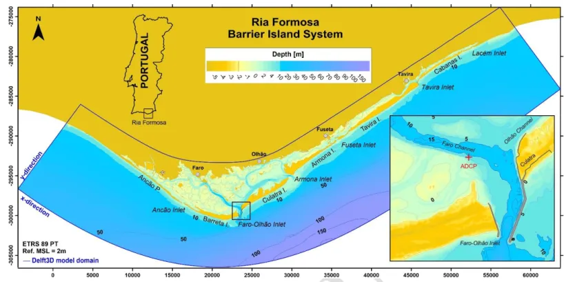
Fig. 1 - Location map of the study region. Zoom rectangle shows the Faro-Olhão Inlet, the location for TEC array deployment, and the red cross shows were the ADCP was deployed.

Tide and wind forcing together with morphological and morphodynamics characteristics of the Ria Formosa inlets control water exchange rates and residual flows of the lagoon [32]. Morphological changes (natural or human) in any of the inlets can modify tidal prism on any other inlet of the system, especially on the inlets of the western sector which have a significant interplay between them [32]. These alterations can have an important repercussion on some of the economic activities of the region such as aquaculture, salt farming, fishing, shellfish farming, shipping, mining, and tourism. These activities have local and regional importance, and the shellfish farming assumes national impact representing 60% of the total Portuguese production. Such a congregation of different activities makes the management of the Ria Formosa a very difficult task for the region’s decision-makers and any relevant change in the hydrodynamics of the system can affect and disturb these activities as a cascade effect.

Measurements of the tidal prism performed between 2006 and 2007 for each inlet of the Ria Formosa reveal a clear circulation pattern between Faro-Olhão and Armona inlets [33]. The two inlets present ebb-dominated behaviour (i.e. higher mean ebb velocity associated with shorter ebb duration). However, at the Faro-Olhão Inlet, the flood prism is considerably greater than the ebb prism. The sediment transport direction is strongly landward (flood) directed as evidenced by the regular dredging operations required to maintain the channel navigability. In contrast, the Armona Inlet is always ebb-dominant and capable of flushing sediment seaward under fair-weather conditions, especially during spring tides. These two major inlets represent almost 90% of the total prism of the Ria Formosa. The interconnection between both inlets is particularly active during spring tides (Faro-Olhão 61% and Armona 23% of overall Ria Formosa tidal-prism), but is reduced during neap-tides when the inlets drain the basin more independently (Faro-Olhão 45% and Armona 40% of overall tidal-prism).

Ria Formosa has a long history of tidal energy harvesting, from the XII to the XX century tide mills have been operating in its channels taking advantage of the periodic fall and rise of the water level. Pacheco et al. [5] determined for a specific cross section of the Faro-Olhão Inlet a

mean and maximum potential extractable power of 0.4 kW.m-2 _{and 5.7 kW.m}-2_{, respectively. By} means of a 2DH numerical model, González-Gorbeña et al. [34] assessed the tidal resource for the whole Faro-Olhão Inlet obtaining tidal current velocities greater than 0.7 m.s-1 _{for more than} 60% of the time at the inlet throat.

3.

The Delft3D is employed as a tool for implementing the SBO methodology (detailed in Section 3.2) to define the optimum TEC array size of the Faro-Olhão Inlet taking into consideration both the resource (i.e. tidal energy) and the environment (i.e. consequences). The model is adopted in a depth averaged mode (2DH), since there is a limited fresh water input into the lagoon and negligible salinity and temperature gradients. The hydrodynamic model is coupled with a morphodynamic model to approximate bed changes as function of sediment transport rates, as exemplified in other studies [35], [36], [37].

The model domain is discretised with a curvilinear orthogonal grid in spherical coordinates that follows the general cuspate shape of the lagoon (Fig. 1), and extends approximately over 60 km alongshore and 18 km cross-shore. The domain is discretised with 1100×462 grid points. The grid resolution varies between Δx = 750 m, Δy = 175 m at the offshore area and Δx = 20 m, Δy = 15 m over the inlet areas, where the grid was refined in order to capture the complex and rapid changing morphology. The model bathymetry was built using the high resolution LiDAR topo-bathymetry performed in 2011, coupled with bathymetric data from the Faro Port Authority and with 2016 bathymetric surveys performed under the SCORE project [38]. The LIDAR and SCORE bathymetries are available online (open-access) at the SCORE project database [39]. Bottom roughness was assigned to each grid point using the White-Colebrook’s formulation [40]. At the ocean boundary, the sea level was prescribed using the main tidal constituents (Table 1). The models time step is 30 s, which, according to the Courant–Friedrichs–Levy criterion [41], is sufficiently small to ensure numerical stability. For calibration and validation purposes, the effect of wind was considered in the simulations as a spatially uniform forcing. The wind time series were retrieved from the meteorological station located in Faro’s airport. Due to the low local wave climate and the narrow nature of the Faro-Olhão Inlet the offshore wave forcing does not significantly affect the array deployment area. For the purpose of this study, the effects of waves and storm surge are not considered in the numerical simulations.

Table 1 - Principal Ria Formosa tidal constituents from TOPEX/POSEIDON-7.2 DATA [64].

Harmonic constant Amplitude (m) Phase (°)

M2 0.995 56.58 S2 0.365 82.57 N2 0.211 39.87 K2 0.098 78.67 K1 0.069 49.75 O1 0.058 310.45 P1 0.020 43.78 Q1 0.017 260.98 MF 0.001 261.36 MM 0.001 191.43

3.1.2. Hydro-morphodynamic model calibration and validation

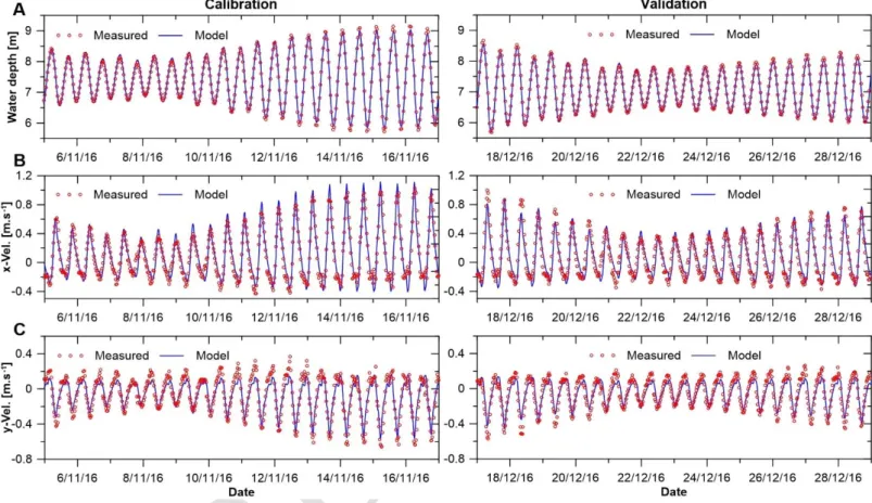
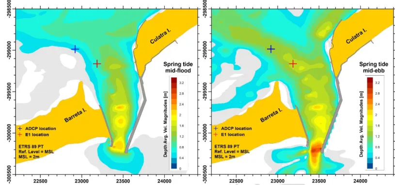
Two sets of hydrodynamic data were used for the hydrodynamic model calibration and validation process. Water levels and flow velocities were obtained with a bottom-mounted ADCP (Nortek Signature 1000). The ADCP (Fig. 1) was deployed at a mean water depth of 7.7 m (Fig. 1) from 03/11/2016 to 17/11/2016 and 14/12/2016 to 02/12/2017 and was set to measure average velocities every 60 s for time intervals of 600 s at 0.2 m vertical cells. Part of those time series have been used to calibrate and validate the model results (Fig. 2). Peak spring flood and ebb tidal current velocities contour maps are illustrated in Fig. 3.

Fig. 2 - Water depth (A), Easting velocity component (B) and Northing velocity component (C) comparisons between measured data (ADCP Nortek Signature1000) and model results (Delft3D) for: calibration (left) and validation data sets (right).

Fig. 3 – Tidal current velocities contours for spring tide mid flood (left) and mid ebb (right).

To assess the model performance several statistical parameters have been calculated. Table 2 summarizes the goodness-of-fit statistics of the model for both calibration and validation data sets. Observing bias values, it is clear that the model output tends to slightly overestimate water levels and underestimate Easting velocity components. For the calibration model, Northing velocity amplitudes show the poorest agreement of the three variables but still with Index of Agreement (IA) and Correlation Factor (R) values around 0.9. In general terms, and taking into account all statistical parameters, the model performance is considered very good. Notice that the underestimation of flow velocities, specially peak flows, will have an implication on the power outputs estimation, which will also be underestimated as it is proportional to the cube of the flow velocity. Furthermore, morphological changes are more sensitive to errors in velocities. Differences between measured and computed data could be related to uncertainties in bathymetric data due to a lack of accurate information of all recent dredging volumes. Possibly also related to a grid size with a degree of refinement not enough to characterize all channels features. Additionally, differences could be also related to the inlet characteristics (composed by the curved ocean and lagoon coast and jetties). Despite the high degree of grid refinement, the Faro-Olhão Inlet presents a high degree of complexity, which it makes difficult to characterise using a curvilinear finite difference grid.

Table 2 - Model Goodness-of-Fit Statistics. Standard Deviation of Residuals (SDR); Normalised Root Mean Square Error (NRMSE), Index of Agreement (IA) and Correlation Coefficient (R).

Statistics

Calibration Validation

Water Level

[m] x-vel [m.s

-1_{] y-vel [m.s}-1_] Water Level

[m] x-vel [m] y-vel [m.s -1_] Bias 0.0006 -0.016 -0.007 0.018 -0.009 0.003 SDR 0.078 0.130 0.116 0.085 0.112 0.072 NRMSE* _{0.007 0.017 0.0226 0.026 0.074 0.070} IA* _{0.998 0.961 0.898 0.997 0.972 0.959} R* _{0.995 0.929 0.901 0.994 0.946 0.947} *_adimensional

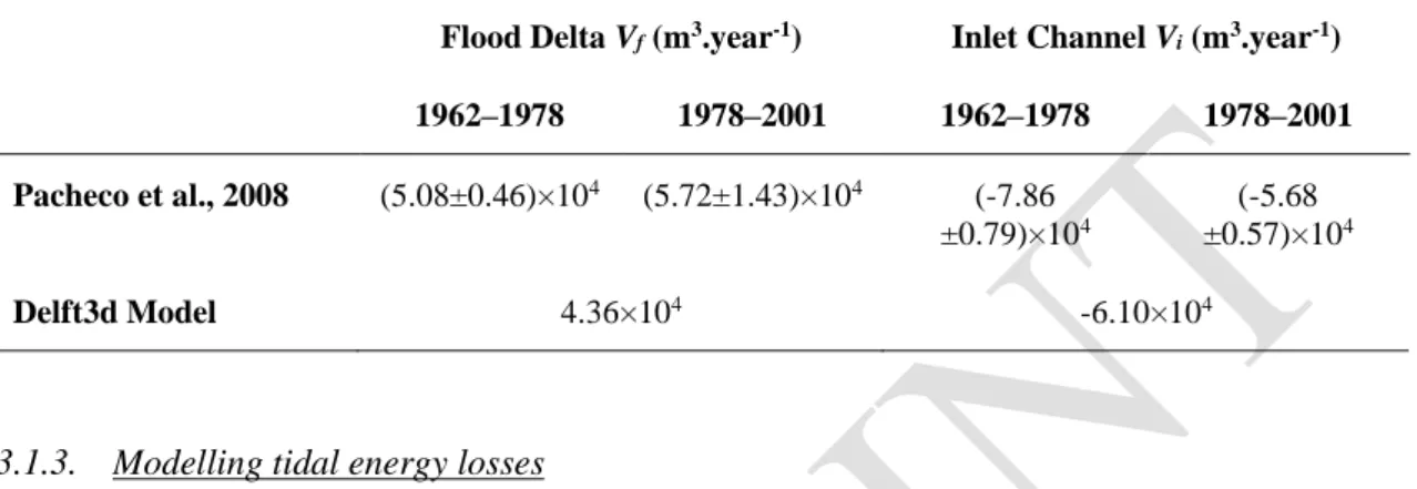
Morphological predictions were simulated with the use of the morphological acceleration parameter (MorFac), assuming the linear hydrodynamic forcing during one morphological step [35], [42]. Regarding the morphodynamic validation, model results were compared with annual estimates of sediment budgets obtained from long-term data collected at the Faro-Olhão Inlet over the period of 1962-2001 [33]. Pacheco et al. [33] estimated the annual sediment budget of Faro-Olhão Inlet (and adjacent areas) from volume computation using available bathymetric data, topography and dredging reports. The authors compared the model results with two periods (e.g. 1962-1978 and 1978-2001), quantifying different sources of uncertainty. The relative advantage of using long-term sediment budget data for model validation, instead of short term detailed bed level changes, is that results are relatively independent of the initial model bathymetry and more representative of the general sediment transport processes and patterns. Two characteristic areas of the Faro-Olhão Inlet were selected for calculating the sediment volume changes (Fig. 4): (i) the flood-tidal delta area (Vf) and (ii) the inlet area (Vi). The adopted approach was developed by combining the use of long-term data to identify sediment transport patterns for model calibration purposes [43], with the sediment budget concept for pre-defined neighbouring cells [44].

Fig. 4 - Aerial photo of the Faro-Olhão Inlet with the outline of the flood tidal delta (Vf , blue) and

the inlet area (Vi, red), used to calibrate the morphodynamic model.

During model calibration, the morphological model was forced with a schematized tide [35], [45] based on the tidal asymmetry between the main diurnal (O1 and K1) and semidiurnal (M2) tidal components and with a morphological acceleration factor, MorFac, of 48. Because both areas are located within the lagoon, the wave effects on sediment transport were assumed negligible. The dominant sediment size found in the flood delta was D50 = 425 μm [46]. The sedimentation and erosion results for both areas (Vf and Vi) together with the long term measured data are presented on Table 3. The estimation for the latter morphological period (1978-2001) provides a better estimate since the flow regimes in the Faro-Olhão and Armona inlets are closer to the conditions described by the present bathymetry.

The model produced good quantitative results with accretion at the flood delta and erosion at the inlet channel, suggesting a good functioning of the model, able to reproduce the main morphological patterns in the vicinity to the inlet. Overall, model values compare favourably in terms of magnitude to the best estimates of accretion/erosion volume obtained by [33] for two different periods. After calibration the morphological simulation was repeated using a smaller

morphological acceleration factor (MorFac = 12) and for various spring-neap tidal cycle. The results of this simulation were in good agreement with the model results obtained with larger MorFac values and schematized tidal forcing, suggesting a good and coherent representation of the sediment patterns by the model. Finally, a MorFac of 26 (equivalent to a period of ~1 year) was adopted for the numerical simulations used during array optimisation.

Table 3 - Accretion/erosion measured and model estimates for both flood delta and inlet channel polygons (Vf and Vi). Error bounds in [33] represent the propagated error associated with the measurement and digitisation uncertainty.

Flood Delta Vf (m3.year-1) Inlet Channel Vi (m3.year-1)

1962–1978 1978–2001 1962–1978 1978–2001 Pacheco et al., 2008 (5.08±0.46)×104 _{(5.72±1.43)×10}4 _(-7.86 ±0.79)×104 (-5.68 ±0.57)×104 Delft3d Model 4.36×104 _-6.10×104

3.1.3. Modelling tidal energy losses

The impact of energy extraction on flow and sediment transport patterns can be simulated by enabling or adding an additional sink/source momentum term in the equations of conservation of momentum to parameterize the extra loss of energy generated by a TEC array in a subgrid-scale. In Delft3D-Flow, the extra loss of energy can be parameterised using a quadratic energy loss term given by: 2 2 2 2 loss u x loss v y C M u u v x C M v u v y − − = − +  = − +  (1)

where Closs depicts the energy loss coefficient; Δx, Δy are the cell widths in the x and y directions, respectively; and u and v the Easting and Northing velocity components. Following the procedure presented in [47], the extra loss of energy can be related with the drag force, FD, exerted in the fluid flow by an array of N TECs. FD is composed of two parts, one due to the support-structure drag, with cross-sectional area As, and another due to the power extraction of the turbines, with a rotor swept area of AT with diameter D, i.e:

(

)

1 2

D s s T T in

F = N C A +C A U (2)

ρ depicts sea water density (1025 kg.m-3_{), C}

s and CT stand for the drag coefficient of the structure, and thrust coefficient of the rotor, respectively, and Uin is the incident flow velocity. Because FD has force units and the momentum source term Mx has acceleration units, and to be able to relate both quantities, it is necessary to divide Eq. (2) by the control volume mass where the TEC is located, e.g. for the x-direction:

(

)

where H is the water column height of the control cell. Here, it is assumed that the incident flow velocity is similar to the flow velocity at the porous plate, which is a valid approximation for a 2DH model, and where the TECs modelled are small compared with the grid cell. In cases where the TEC is similar to the grid cell size, a correction for the CT is needed when it is expressed as a function of the flow velocity at the porous plate [48]. Solving for Closs gives:

(

)

Overall, this approach is similar to those used by other authors, where slight differences may exist depending on how the sink/source term is incorporated in the model and the numerical method employed, i.e. finite difference (e.g. [49]), finite volume (e.g. [13]) and finite element (e.g. [50]). The main difficulty of the approach is to determine the precise value of the drag coefficient of the TEC (i.e. rotor and support-structure) that generates the appropriate head loss, (i.e. wake velocity deficit). For a review on modelling energy extraction in tidal flows refer to [51].

A 1:4th _{scale Evopod device (E35 hereafter) from Oceanflow Energy Ltd. is used for} calculations. The E35 has a diameter of 4.5 m and its semi-submerged support platform has a length of 13 m, beam of 4.5 m, height of 8 m, displacement of 13 tonnes, and a rated output of 35 kW (Table 4). E35 was already tested at Sanda Sound West Scotland at 22 m water depth [47], an area that resembles Ria Formosa in terms of tidal resource and environmental constraints (i.e. depth and current velocities).

Table 4 - Tidal Energy Converter EvopodTM _{E1 and E35 specifications.}

Parameter Values

E1 E35

Rotor diameter, D [m] 1.5 4.5

Length, L [m] 3.5 13

Cut-in speed, Uci [m.s-1] 0.7 0.7

Rated flow speed, Ur [m.s-1] 1.75 2.3

Rated power, Pr [kW] 1 35

Power coefficient, CP [-] 0.28 0.35

Thrust coefficient, CT [-] 0.40 0.40

Swept area, AT [m²] 1.77 15.9

Structure drag coefficient, CS [-] 0.15 0.15

TEC frontal area, AS [m²] 2.03 18.3

Using mooring tension data from an Evopod 1:10th _{scale prototype deployment [52] and by} fitting to the data a quadratic drag law of the form y = Ax2 _{+ b with y = F}

T,x , b = FT,o, x = U; and A = 0.5ρ(CT AT + Cs As) an overall CT is obtained. Values given by the manufacturer for Cs and As, are 0.15 and 2 m2, respectively, resulting in a CT = 0.4. In Fig. 5, it is visible that a fix CT provides a good agreement with measurements. Finally, assuming a similar CT value for the E35 and by using Eq. (4), a Closs is calculated for each cell in the model where TECs are located.

Fig. 5 - Mooring lines tension for the 1 kW Evopod deployed at Faro-Olhão Inlet, Ria Formosa. Those values correlated positively with the fitted quadratic drag law (R2 _{= 0.87).}

3.2. SBO Methodology

3.2.1. Problem formulation and design of computer experiments

In order to formulate an optimisation model, it is necessary to define the objective function to maximise or minimise, the constraints and the design variables involved in the problem. The standard form of a mathematical optimisation model is defined by:

Maximise f0 (x) ;

Subject to: gi (x) ≥ bi, i = 1,…, m; hj (x) = dj, j = 1,…, k;

where the vector x {x1,…,xs} depicts the set of design variables of the problem, the function f0: Rn _{→ R depicts the objective function, the functions g}

i and hj: Rn → R, i = 1,…, m; and j = 1,…, k; depict the inequality and equality constraint functions, and the constants b1,…, bm; and d1,…, dk provides bounds and values of the constraints. In surrogate-based optimisation, the validated surrogate can represent the objective function, i.e. f0 (x) = ŷ (x), or any of the constraints, i.e. g (x) = ĝ (x). Furthermore, there are optimisation models formulated using multiple surrogates as is the case of the present study.

In the TEC array layout problem the design variables are up to the choice of the designer and specific for each case. Several options can be used as expressed in [24], [25]. For the purpose of this study, the TEC layout optimisation problem is formulated as function of two design variables x {x1, x2}, the number of rows of the array (x1) and the number of devices in each row (x2) that maximises the capacity factor of the layout subject to a series of constraints.

Array row characteristics are defined based on the main features of the Faro-Olhão Inlet features (i.e. geometry and water depths), energy resource (i.e. occurrence of flow velocities) and TEC specifications (e.g. rotor diameter, length, etc). The tidal resource in the region is characterised using the validated hydro-morphodynamic model. Fig. 6 shows a contour map of

the Faro-Olhão Inlet region with occurrence of tidal currents with velocities stronger than 0.7 m.s -1_{, which is the cut-in velocity for the E35 turbine. From the contour map, it is evident that the} highest energy resource is at the inlet throat. As a result, the first TEC row is placed at the inlet throat and successive rows are placed inwards with a fixed streamwise spacing between rows of 20D (D, rotor diameter) to allow a reasonable wake recovery, i.e. velocity deficit, U/Uo, ≤ 0.95 [53]. Considering occurrence of tidal currents stronger than the turbine’s cut-in velocity during ~25 % of the time or above, the maximum number of rows is set to 13 composing a maximum array length of 1135 m. TEC rows are placed in regions with depths ≥ 10 m, therefore array rows are not symmetrically aligned across the streamwise axis. Each TEC row has a width of 162 m, which matches the width of the inlet throat. The number of E35 TECs in each row varies from 6 to 11 units, corresponding to a lateral spacing of 6D and 3D, respectively plus 3D of clearance at the tip of the rows. The maximum number of turbines in a row is defined in order to let the rotation of the devices align with the tidal currents, while the minimum number of devices is set to decrease blockage effects.

Fig. 6 – (Left) bathymetry contours and (Right) occurrence of tidal currents with velocities stronger than 0.7 m.s-1 _{for the Faro-Olhão Inlet region. Blue/red crosses denote the ADCP/E1 deployment} locations, the blue lines represent TEC rows and grey lines show the computational grid.

A series of constraints are included in the optimisation model to find the optimum installed capacity of a TEC array without creating significant detrimental environmental impacts on a regional level. The environmental aspects considered for analysis are related with tidal discharges and morphological processes that are detailed in sub-section 3.2.2. Thus, TEC array size, and its effects on flow characteristics and inlets morphology, are described through surrogates built as functions of two integer design variables: the number of rows in the array (x1) and the number of TECs for every row of the array (x2). The intervals of each integer variable are set to: x1 ∈ [1, 13] and x2 ∈ [6, 11].

Once the optimisation model is conceptually formulated, surrogates for the objective function and constraints have to be built. For this purpose, it is necessary to conduct a series of computer simulations to adequately describe the design space. The size of the sample plan should be around ten times the number of design variables as suggested in [54]. Fig. 7 illustrates the sample plan adopted in this study, which consists of 2 factors (i.e. design variables) with 6 and

13 levels each, respectively, and with 15 sample points for each variable giving an experimental design plan size of 30 data points (blue dots). An additional 3 points (red dots) are added for surrogate validation.

Fig. 7 – Normalised [-1 to 1] sample plan design. Blue points represent initial sampling plan and red dots represent validation points. Variables limits: x1∈ [1, 13] TECs and x2∈ [6, 11] rows.

3.2.2. Numerical simulations

The validated numerical model detailed in sub-section 3.1 is employed to execute the 30 cases defined in the sample plan and the 3 validation points shown in Fig. 7. Simulations are run for a fortnight cycle ~14 days, using a morphological time scale factor of 26 to quantify bed-level changes after a period of 364 days (i.e. ~1 year). Here, the effect of wind is discarded. In Appendix A, Table A.1 to Table A.4 summarize the results obtained for the sample plan (cases 1 to 30) and validation points (cases 31 to 33). For each of the simulations the following outputs are obtained: (i) Capacity Factor of the array (CFArray) and of each TEC row within the array (CFi for i = 1,…,13); (ii) percent differences of cumulative flood and ebb instantaneous discharges (ΔƩQi) during a spring tide cycle at each tidal inlet and for the whole lagoon system; (iii) percent differences of the cumulative flood and ebb instantaneous discharges ratio between Armona and the Faro-Olhão inlets (ΔƩQAr / ΔƩQFO); and (iv) net sediment volume changes (ΔV) and differences in average depth changes (Δhavg) for the Faro-Olhão Inlet flood delta and the Armona Inlet.

Due to the fact that the E35 is a floating device, capacity factors for each TEC row were calculated using a transformation of the depth averaged velocity, Ū, obtained by the model simulations, into a flow velocity at rotor centreline, Ur, using a power law of the form:

1/ r z U U H    = _    (5)

where z is the depth of the rotor centreline, i.e. 4 m below water level; β and α are the bed roughness and power law coefficients, with values of 0.4 and 7, respectively. The values of these coefficients have been selected using ADCP data and their values have been maintained constant for the entire array. Then, capacity factors were calculated using Eq (6):

(

)





with Pi and Pr,i depicting the power output and the rated power of i-th array row at the j-th simulation time step, respectively. The analysis of percent differences of cumulative sedimentation/erosion net volume and average gain/loss of depth focuses on the Faro-Olhão and Armona inlets. This decision is based on the following premises: 1) there are no restrictions imposed on the morphological evolution of the Ancão Inlet; 2) near-field effects of TECs on morphodynamics (i.e. red polygon in Fig. 5) are considered not representative due to the numerical model limitations to solve flow-turbine interactions and approximations considered i.e. TECs are modelled as porous-plates in a sub-grid scale using a 2DH approach, where turbine diameter is much smaller than the grid cell size (for a full review of the limitations modelling TECs with Delft3D refer to [51]); and 3) morphodynamic results for Fuseta and Tavira are negligible based on the result of the numerical simulations (Table A.3). For Faro-Olhão and Armona inlets, the morphodynamic responses are computed in the area contained by the polygons defined in Fig. 4 (blue polygon) and Fig. 8, respectively. Both selected polygons represent the areas were expected morphological changes could be higher in association to changes on the hydrodynamic regime, based on the analysis performed by Pacheco et al. [33]. Furthermore, for the Faro-Olhão Inlet, the polygon represents the area used to validate the morphological model and incorporates some of the most valuable geomorphic features of the inlet. For the Armona Inlet, the area within the polygon also defines the navigational channel where cumulative sedimentation/erosion net volumes and depth changes have to be under control.

Fig. 8 - Aerial photo of Armona Inlet. Red line denotes the polygon within which sedimentation/erosion rates are calculated.

3.2.3. Surrogate construction and validation

After the simulations are executed generating the sample data, the surrogates are built. Regarding surrogate selection, there are multiple candidates, each with its advantages and limitations. In order to choose the right surrogate method, Santos [55] describes a series of criteria based on the characteristics of the problem. In the present work, the Radial Basis Function (RBF) method is used because it provides a predictor that passes through all given values of sample points, thus it can express highly non-linear responses. A RBF is a real valued function whose data points, x, are affected on their distance, r, from another data point, xi, named a centre. The distance between the two points is represented by a norm, usually the Euclidian norm, r = ||x – xi||. In this manner, a data point in a data set will affect to a greater extent the nearer points than the faraway points, in such a way that ϕ (x,xi) = ϕ (r) = ϕ (||x – xi||). Thus, the manner in which the distance affects

the data points depends on the basis function selected. In this study, the linear basis,  (r) = r, function is used. For more information on RBF see [56].

Therefore, an approximation response function, ŷi, may be constructed with the form:

(

)



where w is a vector containing the weights, wi, for the linear combination of basis vectors contained in the vector

 with size n

= T_Φ

y w (8)

where y depicts the vector with the computer model responses and  is the matrix enclosing the linear combination of basis vectors.

The values of the weights are estimated using the least squares estimator presented in Eq. (9) ,

(

)

ˆ= _{Φ Φ}T − _ΦT

w y (9)

In this particular study, a total of 26 surrogates are built (i.e. ŷi for i = 1,…,26). While the first surrogate, ŷi for i = 1, depicts the capacity factor of the whole array, surrogates 2 to 14, ŷi for i = 2,..,14, refer to the capacity factor of each array row. Differences in instantaneous cumulative discharges for flood and ebb spring tides of the Faro-Olhão and Armona inlets, the ratio between both (i.e. Armona/Faro-Olhão inlets), and the sum of all inlets are defined by surrogates 15 to 22, ŷi for i = 15,..,22. Finally, surrogates 23 to 26, ŷi for i = 23,..,26, represent the net volume and average bottom depth changes for the Faro-Olhão flood delta and Armona Inlet, respectively.

In order to select the most appropriate basis, each surrogate has to be assessed and validated. The assessment and validation of the surrogate consist in verifying its capacity to predict responses with data points not considered during the regression. For this purpose, a set of three (p = 3) testing points, np, illustrated in Fig. 7, has been selected arbitrarily to carry out a leave-p-out cross validation error method [26],

(

)



To compute the leave-p-out cross validation error, the set of data points N = n + np, is divided into q = N subsets of n = 30 sample points. For each subset, the testing points not considered in the regression are predicted with the surrogate built using the remaining sample points. The leave-p-out method enables to take advantage of the whole set of data points to construct the surrogate model employing the optimal subset of points that minimises the overall error of the model.

The Normalised Root Mean Square Error (NRMSE) and the Normalised Maximum Error (NMAXE) defined by Eqs (12) and (14), are used respectively, to study surrogate’s performance. Forrester et al. [26] suggests that values of a NRMSE < 0.1 and NRMSE < 0.02 imply surrogates with reasonable and excellent predictive capabilities, respectively; i.e.

(

)



Fig. 9 presents the NRMSE and NMAXE results for each of the 26 surrogates built using the technique of cross validation. For all surrogates, NRMSE and NMAXE results are below 0.02. Then, the set of surrogates are used for searching the unexplored design variables space.

Fig. 9 – A) Normalised Root Mean Square Error (NRMSE) and B) Normalised Maximum Error (NMAXE) of surrogates after cross validation.

3.2.4. Optimisation models

Once the surrogates are built, they can be incorporated into the optimisation model representing the objective function and the constraints. Several examples are presented below to illustrate how surrogates can be used in the formulation of an optimisation model to define the size of a TEC array installed in a tidal channel subject to a set of constraints. Depending on the needs and the characteristics of the project, the objective function and constraints can be modified accordingly. Within this study, the values defined for the set of constraints relating array performance and

environmental aspects are presented in Table 5 to Table 7. For instance the CF values refer to the minimum acceptable CF value to consider an array effective. For the discharges the values represent the maximum acceptable discharge change for each inlet and overall system. For the morphological aspects values refer to the maximum accepted changes in volume or vertical shifts at each inlet.

Table 5 – Values of the constraints related with performance aspects of the whole array, CFArray, and of each individual array

row, CFi. Constraint Nº 1 2 3 4 5 6 7 8 9 10 11 12 13 14 Constraint CFArray [%] CF1 [%] CF2 [%] CF3 [%] CF4 [%] CF5 [%] CF6 [%] CF7 [%] CF8 [%] CF9 [%] CF10 [%] CF11 [%] CF12 [%] CF13 [%] Value 12.5 15 12 10 10 10 10 10 10 10 10 10 10 10

Table 6 – Values of the environmental constraints related with flood/ebb spring discharges (ΔƩQ) for Faro-Olhão (FO) and

Armona (Ar) inlets, and their discharges ratio (ƩQAr/ƩQFO). Subscripts f and e depict for flood and ebb tides, respectively.

Constraint Nº 15 16 17 18 19 20 21 22 Constraint ΔƩQf, FO [%] ΔƩQf, Ar [%] ƩQf, Ar/ƩQf, FO [%] ΔƩQf, all [%] ΔƩQe, FO [%] ΔƩQe, Ar [%] ƩQe, Ar/ƩQe, FO [%] ΔƩQe, all [%] Value -10 10 7.5 -5 -5 2.5 2.5 -2.5

Table 7 – Values of the environmental constraints related with morphological aspects. ΔVnet and Δhavg

stand for the net sediment volume and average depth differences, respectively, for Faro-Olhão (FO)

and Armona (Ar) inlets.

Constraint Nº 23 24 25 26

Constraint ΔVnet, FO [m3/yr] ΔVnet, Ar [m3/yr] Δhavg, FO [cm/yr] Δhavg, Ar [cm/yr]

Value -10,000 40,000 -5 15

Model 1

The objective of the first model consists in defining the maximum number of array rows, x1, that can be installed without affecting the environment adversely. These effects are quantified by a set of constraints inequalities, ĝ (x) ≤ b, where ĝ (x) depicts a set of the built surrogates representing the environmental responses (i.e. cumulative discharges, net sedimentation/erosion volumes, etc.), b is a vector containing the values of the restrictions imposed and x is the set of design variables. Notice that each row has associated 6 possible TECs combinations, i.e. for x2 ∈ {6,…,11}, which could yield more than one optimum solution. Therefore, in order to avoid a multiple solution problem, it is necessary to include an additional objective function to be maximised or minimised. This could be, for example, maximise power output or array capacity factor, or even minimise any particular environmental impact. For the purpose of this study, the capacity factor is selected as the second objective function to be maximised, which is again used in models 2 and 3.

Then, the mathematical formulation of the multi-objective optimisation problem is as follows:

Subject to:

ĝi (x) ≥ bi, ∀ i ∈ {15, 18, 19, 22, 23, 25} (16)

ĝi (x) ≤ bi, ∀ i ∈ {16, 17, 20, 21, 24, 26} (17)

x1 ∈ {1,..,13}, x2 ∈ {6,…,11} (18)

Model 2

Similarly to Model 1, there is the possibility to maximise the number of TECs per row, x2, that will not violate the environmental restrictions imposed. This way, the mathematical formulation of Model 2 is as follows: Maximise {x2, CFArray (x)} (19) Subject to: ĝi (x) ≥ bi, ∀ i ∈ {15, 18, 19, 22, 23, 25} (20) ĝi (x) ≤ bi, ∀ i ∈ {16, 17, 20, 21, 24, 26} (21) x1 ∈ {1,..,13}, x2 ∈ {6,…,11} (22) Model 3

Alternatively to models 1 and 2, the problem can be formulated in terms of finding the maximum number of TECs, i.e. x1x2, that the system could handle without violating the environmental constraints: Maximise {x1x2, CFArray (x)} (23) Subject to: ĝi (x) ≥ bi, ∀ i ∈ {15, 18, 19, 22, 23, 25} (24) ĝi (x) ≤ bi, ∀ i ∈ {16, 17, 20, 21, 24, 26} (25) x1 ∈ {1,..,13}, x2 ∈ {6,…,11} (26) Model 4

As models 1 to 3 do not ensure an overall efficient array, there is the possibility to formulate the model in terms of maximising the number of TECs and the total power output of the array but imposing minimum values of efficiency for the whole array as well as for each individual row.

Maximise {x1x2, PArray} (27)

Subject to:

PArray= CFArray (x) x1x2 Pr t (28)

ĝi (x) ≥ bi, ∀ i ∈ {1,…, x2 + 1} (29) (28)

ĝi (x) ≤ bi, ∀ i ∈ {16, 17, 20, 21, 24, 26} (31) (30)

x1 ∈ {1,..,13}, x2 ∈ {6,…,11} (32) (31)

Equations (15), (19), (23) and (27) define the objective functions to be maximized. In Model 4, Pr stands for the rated power of the turbine (35 kW), and the time interval to compute power production (364 days.yr-1_{). Equations (16), (17), (20), (21), (24), (25), (30) and (31)} establish the set of environmental constraints, i.e. the min/max values of the constraints presented in Table 5 to Table 7; while equation (29) designates the set of performance constraints related with minimum allowable capacity factors for the array, and for each row. Equation (28) defines how to calculate the overall power output of the array. Finally, equations (18), (22), (26) and (32) declare the values of the integers variables, i.e. the number of rows and the number of TECs per row. The value of the variable indicating the number of rows implicitly considers which array rows are turned on and off, due to the fact that array rows are placed consecutively with respect to the first row, which is always placed at the inlet throat.

4.

The design variables space are explored through the built surrogates. Responses of each surrogate within the design variables domain are presented graphically in Fig. 10 to Fig. 15. While the Fig. 10 presents the annual power output for all possible TEC arrays, Fig. 11 illustrates the capacity factors for the TEC array as well as for each array row. Outputs are obtained evaluating the surrogates in all possible combinations of the two design variables (i.e. 78 array layouts). From these figures, it is clear that although larger arrays yield higher power outputs, the overall efficiencies are very low. On the other hand, the first rows of the potential arrays (i.e. the one located at the inlet throat) benefit from faster flows yielding higher power outputs than rows positioned further inside the lagoon, where the available tidal resource is lower.

Fig. 10 - Classed post plot presenting array annual power output results for all possible combinations of the two design variables (i.e. 78 array layouts). The plots show that the highest power output is achieved by larger size arrays i.e. with 13 rows and 11 TECs/row. Variables limits are: x1∈ [1, 13] rows and x2∈ [6, 11] TECs per row.

Fig. 11 – Classed post plot presenting capacity factor results of all possible combinations of the two design variables (i.e. 78 array layouts) for the whole array (top left corner) and for each row (row 1 to 13). The plots show that the highest capacity factors are achieved by arrays with few rows (x1 ≤ 5). The effect of the number TECs (x2) varies within each row an in all rows, e.g. in the plot for Row-3, capacity factors are visible larger for cases with 7-9 TECs than for case with 6, 10 and 11 TECs. Variables limits are: x1∈ [1, 13] rows and x2∈ [6, 11] TECs per row.

The power outputs generated and the capacity factors achieved by the set of TECs and rows that form each one of the possible array layouts are plotted in Fig. 12. From this figure, it is visible how power output and capacity factors achieved by the array tend to reach an asymptotic behaviour with increasing turbine number. This behaviour implies that by adding more TECs will

not result in substantial gains on array power production, which is specifically true for arrays size ≥ 120 devices. Moreover, array capacity factor decreases by increasing the number of TECs until it reaches a constant value of around 6%. In Fig. 12A, it is noticeable that the largest variability on power output and capacity factor occurs for arrays with a number of TECs between 36 and 117 units, and between 30 and 90 units, respectively. On the other hand, in Fig. 12B, differences in array power output increase with array size, with values that go from 0.24 GWh.year-1 _{to 0.79} GWh.year-1 _{for arrays with 1 and 13 rows, respectively. This implies that depending on the array} configuration, power outputs can vary significantly for arrays with the same number of TECs. The largest difference (~0.4 GWh.year-1_{) is obtained for an array with 66 TECs, where the array} configuration of 6 rows with 11 TECs per row has better performance that an array with 11 rows and 6 devices per row. Regarding array capacity factor, variability for arrays with same number of rows are not so large and stay within 1% and 1.4%. The largest fluctuations are observed for arrays with 1 row and for mid-size arrays, i.e. arrays with 6 to 7 rows. For arrays with 7 rows, array capacity factors do not always decrease with increasing the number of TECs per row. For this case, the highest capacity factor is obtained when 8 TECs are placed in each row.

Fig. 12 – Array annual power output and capacity factor as a function of both design variables: A) number of TECs, and B) number of rows.

Fig. 13 illustrates these phenomena showing the variability of the tidal resource in terms of power density without TECs and for two array configurations of 13 rows and, 6 and 11 devices, respectively. As can be seen from Fig. 13, the tidal resource varies in each row and decreases further away from the inlet throat, although not linearly. In general, for the two cases presented, the capacity factor is lower for the case with more devices; however the differences between both cases are not proportional in each row.

Fig. 13 – Power densities for each row of a 13 row array with 6 (red crosses) and 11 (black squares) TECs. Blue circles depict the available power densities without the presence of TECs.

The environmental implications on flood/ebb discharges are proportional to the number of TECs. Fig. 14 summarizes these results, by presenting differences of instantaneous cumulative discharges (A and B) and discharge ratios (C) for the Faro-Olhão and Armona inlets, and differences of instantaneous cumulative discharges (D) for all inlets, each of them assessed during flood (right) and ebb (left) tides. As the number of TECs increase, so do their impacts on discharges, which is greater on flood discharges than on ebb discharges. A reduction of the flood instantaneous cumulative discharges for all inlets will decrease the tidal prism of the lagoon, which in turn can influence water levels and water quality inside the lagoon. In regard to sedimentation/erosion system response to array size, the Faro-Olhão and the Armona inlets present different responses. While for the Faro-Olhão Inlet there is a more clear effect of the number of rows on morphological changes, the Armona Inlet is more sensitive to both design variables, i.e. intensify with increasing number of turbines. Sedimentation rates at Faro-Olhão flood delta (Fig. 15, left) decrease with array size, therefore net volume changes, ΔVnet, FO, and average, Δhavg, FO depth bottom changes quantities are negative. This may result as a consequence of the sediment deposition in the Faro-Olhão Inlet (red polygon in Fig. 4) before reaching the actual flood delta (blue polygon in Fig. 4). The decrease of sedimentation rates at the Faro-Olhão delta may affect shellfish activities. Regarding the Armona Inlet (Fig. 15A, right), net volumes, ΔVnet, Ar, follow a similar trend to the tidal discharges i.e. erosion rates increase (positive values) with larger arrays. Similar patterns are observed for average bottom depths, Δhavg, Ar, (Fig. 15B, right) being larger with arrays of more TECs. Larger erosion rates at the Armona Inlet will generate larger deposition volumes at the flood and ebb tidal deltas, which consequently can have effects, for example, in waterways and shellfish regions. In conclusion, due to the hydrodynamic interconnectivity of Ria Formosa lagoon inlets, any changes in the morphology of one inlet, due to changes of water circulation patterns, will impact the adjacent ones [57]. Therefore, any major change will disrupt this fragile equilibrium and alter the Ria Formosa physiography, with implications to all the social and economic activities.

Fig. 14 - Classed post plot presenting: differences of instantaneous cumulative discharges (A and B) and discharge ratios (C) for the Faro-Olhão and Armona inlets, and differences of instantaneous cumulative discharges (D) for all inlets during flood (right) and ebb (left). Results are for all possible combinations of the two design variables (i.e. 78 array layouts). The baseline Armona/Faro-Olhão ratio for flood and ebb discharges are 37.8% and 35.8%, respectively. Variables limits are: x1∈ [1, 13] rows and x2∈ [6, 11] TECs per row.

Fig. 15 - Classed post plot presenting: A) sedimentation/erosion net volume differences and B) average depth changes for the Faro-Olhão flood delta (left) and Armona inlet (right). Results are for all possible combinations of the two design variables (i.e. 78 array layouts. Positive and negative values indicate increase and decrease of scalar quantities, respectively. While the Faro-Olhão flood delta experiences sedimentation, the Armona Inlet erosion. Variables limits are: x1∈ [1, 13] rows and

x2∈ [6, 11] TECs.

4.2. Optimisation models results

Solving the expressed models (Section 3.2.4), optimum solutions are obtained in compliance with the constraints imposed. Optimisation models are solved employing the enumeration method [58], which evaluates all possible combinations of the discretised design variables space. For each of the optimisation models, Table 8 shows the type of constraints considered (i.e. environmental and performance constraints), the value of the objective function (i.e. the optimum solution), the value of the design variables, the total number of TECs, the capacity factor of the array and its associated power output, while Table 9 to Table 11 present the values obtained for the sets of constraints. Table 8 – Optimum solutions for each model. Results present the values for both design variables, objective function, capacity factor, CFArray, and power output, PArray, of the array. Constraints are

classified as environmental (Envi.) and performance (Perf.)

Model Constraints considered x1 [rows] x2 [TECs/row] Nº TECs Objective function CFArray [%] PArray [GWh.yr-1_] 1 Env. 5 6 30 5 11.4 1.01 2 Env. 1 11 11 11 16.9 0.57 3 Env. 3 11 33 33 12.4 1.25 4 Env. + Perf. 3 10 30 30 12.6 1.20

Table 9 – Capacity factors obtained for the optimum solution of each model. Note that Model 4 is the only model that has performance requirements. Constraint Model CFArray [%] CF1 [%] CF2 [%] CF3 [%] CF4 [%] CF5 [%] CF6 [%] CF7 [%] CF8 [%] CF9 [%] CF10 [%] CF11 [%] CF12 [%] CF13 [%] 1 11.4 16.1 12.0 9.9 10.6 8.6 --- --- --- --- --- --- --- --- 2 16.9 16.9 --- --- --- --- --- --- --- --- --- --- --- --- 3 12.4 15.3 12.0 9.9 --- --- --- --- --- --- --- --- --- --- 4 12.6 15.3 12.2 10.1 --- --- --- --- --- --- --- --- --- ---

Table 10 – Discharge constraints values obtained with the optimum solution. ΔƩQ represents the flood/ebb spring tide discharges for Faro-Olhão (FO) and Armona (Ar) inlets, and ƩQAr/ƩQFO their discharges ratio. Subscripts f and e depict for flood

and ebb tides, respectively.

Constraint Model ΔƩQf, FO [%] ΔƩQf, Ar [%] ƩQf, Ar/ƩQf, FO [%] ΔƩQf, all [%] ΔƩQe, FO [%] ΔƩQe, Ar [%] ƩQe, Ar/ƩQe, FO [%] ΔƩQe, all [%] 1 -7.3 7.0 5.9 -2.7 -3.0 1.0 1.5 -1.4 2 -3.1 3.3 2.5 -1.0 -0.9 0.1 0.4 -0.5 3 -8.7 7.5 6.8 -3.4 -4.1 1.2 2.0 -1.9 4 -9.4 7.8 7.1 -3.7 -4.0 1.0 1.9 -1.9

Table 11 – Morphological constraints values obtained with the optimum solution. ΔVnet and Δhavg

stand for the net sediment volume and average depth differences, respectively, for Faro-Olhão (FO)

and Armona (Ar) inlets.

Constraint

Model ΔVnet, FO [m3.yr-1] ΔVnet, Ar [m3.yr-1] Δhavg, FO [cm.yr-1] Δhavg, Ar [cm.yr-1]

1 -9475 33262 -0.8 7.5

2 -5250 13390 -0.6 3.2

3 -1232 35561 0.3 8.0

4 -3013 37019 0.1 8.4

Under the constraints imposed, the results from the optimisation models reveal that 5 rows is the maximum allowable number of rows in a TEC array for the Faro-Olhão Inlet without adversely affecting the environment. For this particular case, each row contains 6 devices, resulting in a 30 turbine array. The associated power output of the array is of 1.01 GWh.year-1 operating at a capacity factor of 11.4% (Table 8). The performance of three of the array rows is higher than 10% except for the third row, which is slightly lower (9.9%) and for the fifth row drops to 8.6% (Table 9). On the other hand, the maximum capacity factor is obtained for the first row reaching 16.1%. The lower capacity factor of row 5 is due to two main reasons: i) flow velocities are higher and stronger for most of the time at the throat of the inlet than in any other row of the potential array; and ii) due to depth constraints (TECs have to be positioned in regions with depths ≥ 10 m), from the fifth row onwards, array rows have to be positioned aligned with the tidal channel causing the fastest flow on the ebb tide to miss these rows and to go straight to the fourth row. Then, row number 3, which is affected by the wakes of the second and fourth rows, sees its capacity factor (9.9%) slightly reduced when compared to these two other rows. The most compromised discharge constraint (Table 10) is the Armona and Faro-Olhão flood discharge ratio attaining a 5.9% difference with a constraint value set to 7.5%, while the less compromised is the Armona ebb discharge with a 1% difference with a constraint value set to 2.5%. Concerning the morphological constraints (Table 11), the solution of Model 1 produces the largest impact in terms of deposition rates in the Faro-Olhão’s flood delta, almost attaining the limit of 10,000 m.yr-1_{, while the effects on Armona’s Inlet erosion rates are 17% less than the} limit imposed (i.e. 40,000 m3_{). The optimum array solution of Model 1 does not jeopardise} significantly the morphological constraints.

In Model 2, the maximum number of TECs per row in an array is 11, which is restricted to an array of just 1 row (Table 8). The capacity factor attained by this configuration is the highest of the four models reaching up to 16.9% (Table 9). Obviously, power outputs are the lowest (0.57 GWh.year-1_{), as a consequence of just operating 11 turbines. The impacts on discharges are the} lowest of the four models with results comprising 4% (i.e. Armona ebb discharge) to 33% (i.e. Faro-Olhão flood discharge, and Armona and Faro-Olhão flood discharge ratio) of the constraints.