Sequences of Primitive and Non-primitive BCH Codes

www.scielo.br/tema

doi: 10.5540/tema.2018.019.02.0369

Sequences of Primitive and Non-primitive BCH Codes

A.S. ANSARI1, T. SHAH1, ZIA-UR-RAHMAN1and A.A. ANDRADE2

Received on March 27, 2017 / Accepted on March 21, 2018

ABSTRACT. In this work, we introduce a method by which it is established that how a sequence of non-primitive BCH codes can be obtained by a given primitive BCH code. For this, we rush to the out of routine assembling technique of BCH codes and use the structure of monoid rings instead of polynomial rings. Accordingly, it is gotten that there is a sequence{C_bj_n}1≤j≤m, wherebjnis the length ofCbj_n, of

non-primitive binary BCH codes against a given binary BCH codeCnof lengthn. Matlab based simulated algorithms for encoding and decoding for these type of codes are introduced. Matlab provides in routines for construction of a primitive BCH code, but impose several constraints, like degreesof primitive irreducible polynomial should be less than 16. This work focuses on non-primitive irreducible polynomials having degreebs, which go far more than 16.

Keywords: Monoid ring, BCH codes, primitive polynomial, non-primitive polynomial.

1 INTRODUCTION

Introducing more general algebraic structures lead to various gains in coding applications and the generality of the algebraic structures helps to find more efficient encoding and decoding algo-rithms for known codes. This has motivated special attention of many researchers in considering ideals of certain rings [1], [5], [6], [9] and [10]. The extension of a BCH code embedded in a semigroup ring was considered by Cazaran in [4]. More information regarding ring constructions and its corresponding polynomial codes were given by Kelarev [5]. In [1], the authors elaborated cyclic, BCH, Alternant, Goppa and Srivastava codes over finite rings, which are constructed through a polynomial ring in one indeterminate. Several classes of cyclic codes constructed using the monoid rings are discussed in [2], [14], [13], [12], [11] and [15]. These constructions address the error correction and the code rate in a good way. In [16], Shah et al., showed the existence of a binary cyclic code of length(n+1)nsuch that a binary BCH code of lengthn is embed-ded in it. Though they were not succeeembed-ded to show the existence of binary BCH code of length

*Corresponding author: Antonio A. Andrade – E-mail: antonio.andrade@unesp.br

1Department of Mathematics, Quaid-i-Azam University, Islamabad, Pakistan. E-mail: asia ansari@hotmail.com; stariqshah@gmail.com; ziaagikian@gmail.com

(n+1)ncorresponding to a given binary BCH code of lengthn. In [17], a construction method is given by which cyclic codes are ideals inF2[x;aZ0]n,F2[x]an,F2[x;abZ0]bnandF2[x;1bZ0]abn,

whereZ0is the set of non-negative integers,a,b∈Zanda,b>1. These codes are capable of

correcting random as well as burst errors. Moreover, a link between all these codes are also been developed. Furthermore, in [3], the work of [16] is improved and an association between primi-tive and non-primiprimi-tive binary BCH codes is obtained by using the monoid ringF2[x;a_bZ0], where a,b>1. It is noticed that the monoid ringF2[x;a_bZ0]does not contain the polynomial ringF2[x]

fora>1. To handle this situation, a BCH code in the monoid ringF2[x;aZ0]is constructed and then the existence of a non-primitive BCH code in the monoid ringF2[x;a_bZ0]is showed. The non-primitive BCH codeCbn in the monoid ringF2[x;abZ0]is of lengthbnand generated by a

generalized polynomialg(xab)∈F2[x;a

bZ0]of degreebr. In this line, corresponding to a binary

BCH codeCnof lengthngenerated by a generalized polynomialg(xa)∈F2[x;aZ0]of degreer

it is constructed a codeCbnsuch thatCnis embedded inCbn.

This work extends the work of [3], where the monoid ringF2[x;_bajZ0], withb=a+i, 1≤i,j≤m, wheremis a positive integer, is used. Corresponding to the sequence{F2[x;_bajZ0]}j≥1of monoid

rings, we obtain a sequence of non-primitive binary BCH codes{Cj

bj_n}j≥1, based on a primitive BCH codeCnof lengthn. The non-primitive BCH codeC_bjj_nin the monoid ringF2[x;_bajZ0]is

of length bjn and generated by a generalized polynomialg(x a

b j)∈F2[x; a

bjZ0] of degreebjr. Similarly, corresponding to a given binary BCH codeCnof lengthngenerated by a polynomial

g(xa)∈F2[x;aZ0]of degreerit is constructed a codeCj

bj_nsuch thatCnis embedded inC_bjj_n, where the length of the binary BCH codeCj

bj_nis well controlled with better error correction capability. Along with the construction of a sequence{Cj

bj_n}j≥1of non-primitive binary BCH

codes our focus is on its simulation as well, where the simulation is carried out usingMatlab. It provides built in routines only for primitive BCH codes with degree of primitive polynomial less than 16. Whereas in constructing non-primitive BCH codes, the degree of non-primitive polynomial goes beyond 16, where to overcome this situationGeneric Algorithmis developed in Matlab. The whole method of the algorithm is carried out in two major steps: I) Generating non-primitive polynomial and II) Error correction in received polynomial. In Table 5, some examples are listed. The non-primitive BCH codes with same code rate and error corrections are found to be interleaved codes. By interleaving at random error correcting(n,k)code to degreeβ, we obtain a(βn,βk)code which is capable of correcting any combination oft bursts of lengthβ or less [7, Section 9.4], where the non-primitive BCH codesCj

bj_nhave burst error correction capability along with the random error correction.

2 BCH CODES INF2[X;_BAJZ0]BJ_N, WHERE1≤J≤M.

The set of all finitely nonzero functions f from a commutative monoid(S,∗)into the binary fieldF2is denoted byF2(S). This setF2(S)is a ring with respect to binary operations addition

t∗u=sand it is understood that in the situation wheresis not expressible in the formt∗ufor anyt,u∈S, then(f g)(s) =0. The ringF2(S)is known as themonoid ringofSoverF₂and it is represented byF2[x;S]wheneverSis an additive monoid. A nonzero element f ofF2[x;S]is uniquely represented in the canonical form∑n_i=1f(si)xsi =∑ni=1fixsi, where fi6=0 andsi6=sj

fori6=j. The monoid ringF2[x;S]is a polynomial ring in one indeterminate ifS=Z0.

The indeterminate of generalized polynomials in monoid rings F2[x;aZ0]andF2[x;_bajZ0] are

given by xa andx a

b j _{for each 1}≤ _j≤_{m, wherem is a fix positive integer, and they behave} like an indeterminatexinF2[x]. The arbitrary elements inF2[x;aZ0]andF2[x;_bajZ0]are written,

respectively, asf(xa) =1+(xa)+(xa)2_{+· · ·+(x}a₎n_{andf(xb j}a _{) =1+(xb j}a_{)+(xb j}a ₎2_{+· · ·(xb j}a ₎n_.

The monoidsaZ0and_bajZ0are totally ordered, so degree and order of elements ofF2[x;aZ0]and F2[x;_bajZ0]are defined.

AsF2[x;aZ0]⊂F2[x], it follows that the construction of BCH code in the factor ringF2[x;aZ0]n

is similar to the construction of a BCH code inF2[x]n. Whereas the construction of BCH codes

inF2[x;_bajZ0]/((x a

b j)bjn−1)≡F2[x; a

bjZ0]bj_nis based on the values ofb. BCH codes of length bjninF2[x;_bajZ0]bj_n, corresponding to a BCH codeCnof lengthndon’t exist for all values ofb,

whereb=a+i, such that 1≤i≤m, anda,mare positive integers. For that, consider the fol-lowing mapp(xa_{) =p}

0+p1xa+· · ·+pn−1(xa)n−17→p0+p1(x

a

b j)bj+· · ·+p_n−1(x a

b j)bj(n−1)=

p(x a

b j)_{, which convert a primitive polynomial p}(_xa)_{of degreesinF}2[_x;aZ0]_{to a polynomial} p(x

a

b j)of degree_bj_sinF2[x; a

bjZ0]. This converted polynomial is found to be non-primitive, but is irreducible for some values ofb. Therefore, for the construction of a non-primitive BCH code inF2[x;_bajZ0]bj_n, only this specific value ofbis selected for which there is an irreducible

poly-nomial p(xb ja)_inF2[_x; a

bjZ0]. Thus, for positive integerscj,dj andbjn such that 2≤dj≤bjn

withbjnis relatively prime to 2, there exists a non-primitive binary BCH codeC_bj_n of length bj_{n, whereb}j_{nis order of an elementα∈F}

2b j s.

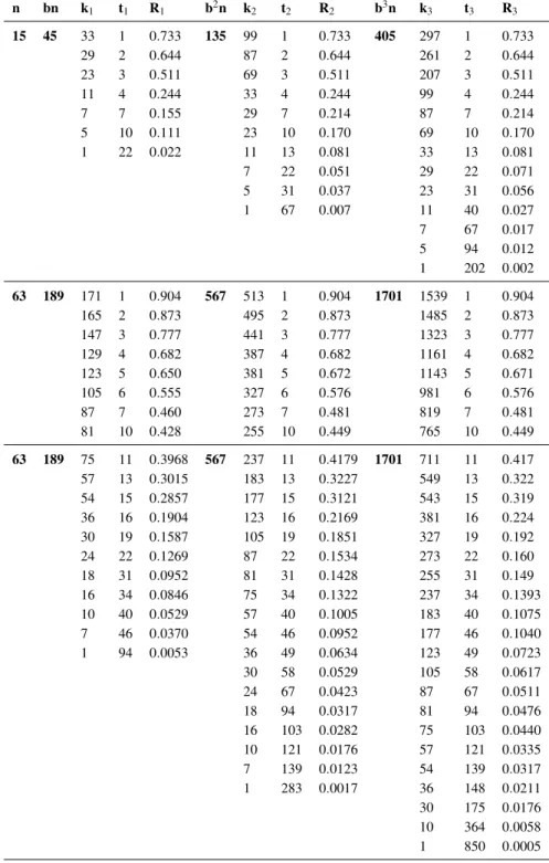
In Table 1, we present a list of irreducible polynomials of degreebj_sinF2[x; a

bjZ0] correspond-ing to primitive irreducible polynomial of degreesinF2[x;aZ0], where forp(xa)∈F2[x;aZ0], p(xab)∈F2[_x;a

bZ0],p(x a

b2)∈F2[_x;a

bZ0], replacexa,x a b _andx

a

b2 _byx,_{yandz, respectively.}

Proposition 1.[3, Proposition 2] If p(xa)∈F2[x;aZ0]is a primitive irreducible polynomial of degree s∈ {2l,3l,4l,6l}, where l∈Z0, then the corresponding generalized polynomial p(x

a b j)of

degree bjs inF2[x;_bajZ0]is non-primitive irreducible for b∈ {3,7,{3,5},{3,7}}, respectively.

Theorem 2. [3, Theorem 3] Let n=2s−1 be the length of a primitive BCH code Cn, where

p(xa)∈F2[x;aZ0]is a primitive irreducible polynomial of degree s such that p(x a

b j)∈F2[_x; a bjZ0] is a non-primitive irreducible polynomial of degree bj_s.

1. For positive integers cj,dj,bjn such that2≤dj≤bjn and bjn are relatively prime to2,

there exist a non-primitive binary BCH code C_bj_nof length bjn, where bjn is the order of an elementα∈F

Table 1: Irreducible polynomials of degree bjs inF2[x;_bajZ0] corresponding to primitive irreducible polynomial of degreesinF2[x;aZ0].

p(xa_{)∈F2[x;aZ0] p(x}a_b)∈F2[x;a

bZ0] p(x a

b2)∈F2[x;a bZ0]

1+ (xa) + (xa)3 _{1+ (x}a₇₎7_{+ (x}a₇₎21 _{1+ (x49}a₎49_{+ (x49}a₎147

1+ (xa3)3+ (_xa3)12

1+ (xa5)5+ (_xa5)20

1+ (xa9)9+ (_xa9)36

1+ (x25a)25+ (_x25a)100

1+ (xa₎3_{+ (x}a₎4 1+ (x

a

3)9+ (_xa3)12

1+ (xa5)15+ (_xa5)20

1+ (xa9)27+ (_xa9)36

1+ (x25a)75+ (_x25a)100

1+ (xa) + (xa)6 1+ (x

a

3)3+ (_xa3)18

1+ (xa7)7+ (_xa7)42

1+ (xa9)9+ (_xa9)54

1+ (x49a)49+ (_x49a)294

1+ (xa_{) + (x}a₎3 +(xa)5_{+ (x}a₎8

1+ (xa3)3+ (_xa3)9+

(xa3)15+ (x

a

3)24

1+ (xa5)5+ (_xa5)15+

(xa5)25+ (_xa5)40

1+ (xa9)9+ (_xa9)27+

(xa9)45+ (x

a

9)72

1+ (x25a)25+ (_x25a)75+

(x25a)125+ (_x25a)200

1+ (xa)4_{+ (x}a₎9 1+ (x

a

7)28+ (_xa7)63

1+ (x49a)196+ (_x49a)441

..

. ... ...

2. The non-primitive BCH code C_bj_nof length bjn is defined as

C_bj_n={v(x a

b j)∈F2[_x; a

bjZ0]bj_n:v(αi) =0for all i=cj,cj+1,· · ·,cj+dj−2.

Equivalently, C_bj_nis the null space of the matrix

H=



    

1 αcj _α2cj _{· · · α}(bn−1)cj 1 αcj+1 _α2(cj+1) _{· · · α}(bn−1)(cj+1)

..

. ... ... . .. ...

1 αcj+dj−2 _α2(cj+dj−2) _{· · · α}(bn−1)(cj+dj−2) 

     .

The following example illustrates the construction of a non-primitive BCH code of length 32n throughF2[x;₃22Z0].

Example 2.1.Corresponding to a primitive polynomial p(x2) =1+ (x2) + (x2)4_{inF2[x; 2Z0]}

there is a non-primitive irreducible polynomial p(x322 ) =1+ (x 2 9)9+ (x

2

9)36inF2[x; 2

1). Letα ∈GF(236)such thatα satisfies the relationα36_+α9_{+1=0. Using this relation, in}

the Table 2, we obtain the distinct elements of GF(236).

By Table 2, it follows that b2n=32×15=135. Now, to calculate the generating polynomial g(x29), first calculate the minimal polynomials. By [8, Theorem 4.4.2], the following roots

α,α2_,α4_,α8_,α16_,α32_,α64_,α128_,α121_,α107_,α79_,α23_,α46_,α92_,α49_,α98_,α61_,α122_,

α109_,α83_,α31_,α62_,α124_,α113_,α91_,α47_,α94_,α53_,α106_,α77_,α19_α38_,α76_,α17_,α34_,α68

have same minimal polynomial m1(x29_{) =p(x}29_{) =1+ (x}92₎9_+(x29₎36_{. It m3(x}29_{)is the minimal}

polynomial forα3_{, thenα}3_,α6_,α12_,α24_,α48_,α96_,α57_,α114_,α93_,α51_,α102_andα69_{all are roots}

for m3(x29_{). Therefore, it follows that m3(x}29_{) = (x}29₎12_+(x29₎3_{+1. Similarly,}

m5(x29_{) = (x}29)

18

+(x29₎9_+1,m 7(x

2

9_{) = (x}

2 9₎36_+(x

2 9₎27₊₁

m₉(x29_{) = (x}29)

4

+(x29_{) +1,m15(x}29_{) = (x}29₎6_+(x29₎3₊₁

m₂₁(x29_{) = (x}29)

12

+(x29₎9₊₁

m₂₇(x29_{) = (x}29)

4

+(x29₎3_+(x92₎2_+(x29_{) +1}

m₄₅(x29_{) = (x}29)

2

+(x29_{) +1,m} 63(x

2

9_{) = (x}29₎4_+(x29₎3_+1.

The BCH code with d2=3has generator polynomial g(x

2

9_{) =1+ (x}29₎9_+(x29₎36_{. It corrects up}

to1error and its code rate is₁₃₅99 =0.733. The BCH code with d2=5has generator polynomial

g(x29_{) = (m}

1(x

2 9_))(m

3(x

2

9_{)) = ((x}

2 9₎36_+(x

2

9₎9_+1)((x 2 9₎12_+(x

2 9₎3₊₁₎

= (x29₎48_+(x92₎39_+(x29₎36_+(x29₎21_+(x29₎9_+(x29₎3_+1.

It corrects up to3errors and its code rate is ₁₃₅87 =0.644. Similarly, the BCH codes with d2=

7,9,15,21,27,45,63and135have generator polynomials

g(x29) = (m 1(x 2 9))(m 3(x 2 9))(m 5(x 2 9))

= (x29₎66_+(x 2 9₎54_+(x

2 9₎45_+(x

2 9₎36_+(x

2 9₎30_+(x

2 9₎27_+(x

2 9₎12_+(x

2 9₎3_+1.

g(x29) = (m₁(x 2 9))(m 3(x 2 9))(m 5(x 2 9))(m 7(x 2 9))

= (x29)102+(x 2 9)93+(x

2 9)90+(x

2 9)57+(x

2 9)48+(x

2 9)45+(x

2 9)12+(x

2 9)3+₁.

g(x29_{) = (m1(x} 2 9_))(m 3(x 2 9_))(m 5(x 2 9_))(m 7(x 2 9_))(m 9(x 2 9₎₎

= (x29₎106_+(x29₎103_+(x29₎102_+(x29₎97_+(x29₎93_+(x29₎91_+(x29₎90_+(x29₎61

+(x29)58+(x 2 9)57+(x

2 9)52+(x

2 9)48+(x

2 9)46+(x

2 9)45+(x

2 9)16+(x

2 9)13

+(x29₎12_+(x29₎7_+(x29₎3_+(x29_{) +1.}

g(x29) = (m₁(x 2 9))(m 3(x 2 9))(m 5(x 2 9))(m 7(x 2 9))(m 9(x 2 9))(m 15(x 2 9))

= (x29)112+(x 2 9)108+(x

2 9)105+(x

2 9)102+(x

2 9)100+(x

2 9)99+(x

2 9)94+(x

2 9)91

+(x29₎90_+(x29₎67_+(x29₎63_{+ (x}29₎60_+(x29₎57_+(x29₎55_+(x29₎54_+(x29₎49

+(x29)46+(x 2 9)45+(x

2 9)22+(x

2 9)18+(x

2 9)15+(x

2 9)12+(x

2 9)10+(x

2 9)9

Table 2: Distinct elements ofGF(236).

α36_=1+α9 _α62_=α26_+α35 _α88_=α16_+α34 _α114_=α6_+α15_+α24_+α33

α37_=α+α10 _α63_=1+α9_+α27 _α89_=α17_+α35 _α115_=α7_+α16_+α25_+α34

α38_=α2_+α11 _α64_=α+α10_+α28 _α90_=1+α9_+α18 _α116_=α8_+α17_+α26_+α35

α39_=α3_+α12 _α65_=α2_+α11_+α29 _α91_=α+α10_+α19 _α117_=1+α18_+α27

α40_=α4_+α13 _α66_=α3_+α12_+α30 _α92_=α2_+α11_+α20 _α118_=α+α19_+α28

α41_=α5_+α14 _α67_=α4_+α13_+α31 _α93_=α3_+α12_+α21 _α119_=α2_+α20_+α29

α42_=α6_+α15 _α68_=α5_+α14_+α32 _α94_=α4_+α13_+α22 _α120_=α3_+α21_+α30

α43_=α7_+α16 _α69_=α6_+α15_+α33 _α95_=α5_+α14_+α23 _α121_=α4_+α22_+α31

α44_=α8_+α17 _α70_=α7_+α16_+α34 _α96_=α6_+α15_+α24 _α122_=α5_+α23_+α32

α45_=α9_+α18 _α71_=α8_+α17_+α35 _α97_=α7_+α16_+α25 _α123_=α6_+α24_+α33

α46_=α10_+α19 _α72_=1+α18 _α98_=α8_+α17_+α26 _α124_=α7_+α25_+α34

α47_=α11_+α20 _α73_=α+α19 _α99_=α9_+α18_+α27 _α125_=α8_+α26_+α35

α48_=α12_+α21 _α74_=α2_+α20 _α100_=α10_+α19_+α28 _α126_=1+α27

α49_=α13_+α22 _α75_=α3_+α21 _α101_=α11_+α20_+α29 _α127_=α+α28

α50_=α14_+α23 _α76_=α4_+α22 _α102_=α12_+α21_+α30 _α128_=α2_+α29

α51_=α15_+α24 _α77_=α5_+α23 _α103_=α13_+α22_+α31 _α129_=α3_+α30

α52_=α16_+α25 _α78_=α6_+α24 _α104_=α14_+α23_+α32 _α130_=α4_+α31

α53_=α17_+α26 _α79_=α7_+α25 _α105_=α15_+α24_+α33 _α131_=α5_+α32

α54_=α18_+α27 _α80_=α8_+α26 _α106_=α16_+α25_+α34 _α132_=α6_+α33

α55_=α19_+α28 _α81_=α9_+α27 _α107_=α17_+α26_+α35 _α133_=α7_+α34

α56_=α20_+α29 _α82_=α10_+α28 _α108_=1+α9_+α18_+α27 _α134_=α8_+α35

α57_=α21_+α30 _α83_=α11_+α29 _α109_=α+α10_+α19_+α28 _α135₌₁

α58_=α22_+α31 _α84_=α12_+α30 _α110_=α2_+α11_+α20_+α29

α59_=α23_+α32 _α85_=α13_+α31 _α111_=α3_+α12_+α21_+α30

α60_=α24_+α33 _α86_=α14_+α32 _α112_=α4_+α13_+α22_+α31

g(x29) = (m₁(x 2 9))(m 3(x 2 9))(m 5(x 2 9))(m 7(x 2 9))(m 9(x 2 9))(m₁₅(x

2 9))(m

21(x 2 9))

= (x29₎124_+(x 2 9₎121_+(x

2 9₎120_+(x

2 9₎109_+(x

2 9₎106_+(x

2 9₎105_+(x

2 9₎94_+(x

2 9₎91

+(x29)90+(x 2 9)79+(x

2 9)76+(x

2 9)75+(x

2 9)64+(x

2 9)61+(x

2 9)60+(x

2 9)49

+(x29)46+(x 2 9)45+(x

2 9)34+(x

2 9)31+(x

2 9)30+(x

2 9)19+(x

2 9)16+(x

2 9)15

+(x29₎4_+(x29_{) +1.}

g(x29) = (m₁(x 2 9))(m 3(x 2 9))(m 5(x 2 9))(m 7(x 2 9))(m 9(x 2 9))(m 15(x 2 9))(m 21(x 2 9))(m 27(x 2 9))

= (x29)128+(x 2 9)127+(x

2 9)126+(x

2 9)124+(x

2 9)120+(x

2 9)113+(x

2 9)112+(x

2 9)111

+(x29₎109_+(x29₎105_+(x29₎98_+(x29₎97_+(x92₎96_+(x29₎94_+(x29₎90_+(x29₎83_+(x29₎82

+(x29)81+(x 2 9)79+(x

2 9)75+(x

2 9)68+(x

2 9)67+(x

2 9)66+(x

2 9)64+(x

2 9)60+(x

2 9)53

+(x29₎52_+(x 2 9₎51_+(x

2 9₎49_+(x

2 9₎45_+(x

2 9₎38_+(x

2 9₎37_+(x

2 9₎36_+(x

2 9₎34_+(x

2 9₎30

+(x29₎23_+(x29₎22_+(x92₎21_+(x29₎19_+(x29₎15_+(x29₎8_+(x29₎7_+(x29₎6_+(x29₎4_+1.

g(x29) = (m₁(x 2 9))(m 3(x 2 9))(m 5(x 2 9))(m 7(x 2 9))(m 9(x 2 9))(m 15(x 2 9))(m 21(x 2 9

))(m₂₇(x29))(m₄₅(x 2 9))=(x

2 9)130+(x

2 9)128+(x

2 9)125+(x

2 9)124+(x

2 9)122

+(x29₎121_+(x 2 9₎120_+(x

2 9₎115_+(x

2 9₎113_+(x

2 9₎110_+(x

2 9₎109_+(x

2 9₎107

+(x29₎106_+(x29₎105_+(x29₎100_+(x92₎98_+(x29₎95_+(x29₎94_+(x29₎92

+(x29)91+(x 2 9)90+(x

2 9)85+(x

2 9)83+(x

2 9)80+(x

2 9)79+(x

2 9)77+(x

2 9)76

+(x29₎75_+(x29₎70_+(x29₎68_+(x29₎65_+(x29₎64_+(x29₎62_+(x29₎61_+(x29₎60

+(x29)55+(x 2 9)53+(x

2 9)50+(x

2 9)49+(x

2 9)47+(x

2 9)46+(x

2 9)45+(x

2 9)40

+(x29₎38_+(x 2 9₎35_+(x

2 9₎34_+(x

2 9₎32_+(x

2 9₎31_+(x

2 9₎30_+(x

2 9₎25

+(x29₎23_+(x29₎20_+(x29₎19_+(x29₎17_+(x29₎16_+(x29₎15_+(x29₎10_+(x29₎8

+(x29)5+(x 2 9)4+(x

2 9)2+(x

2 9) +₁.

g(x29_{) = m1(x} 2 9_))(m 3(x 2 9_))(m 5(x 2 9_))(m 7(x 2 9_))(m 9(x 2 9_))(m 15(x 2 9₎₎

(m₂₁(x29_))(m 27(x 2 9_))(m 45(x 2 9_))(m 63(x 2 9₎₎

= (x29)134+(x 2

9)133+· · ·+ (x 2 9)2+(x

2 9) +₁.

Finally, errors like3,4,7,10,13,22,31and67are corrected.

From Example 2.1 and [3, Example 1], it follows that the code generated throughF2[x;_bajZ0] corrects more errors and has better code rate than the code generated throughF2[x;aZ0]. Now, we are in position to develop a link between a primitive(n,n−r)binary BCH codeCnand a

non-primitive(bjn,bjn−rj)binary BCH codeCbj_n, whererandrjare, respectively, the degrees of

their generating polynomialsg(xa)andg(x a

b j)_{. From Theorem 2, it follows that the generalized} polynomialg(xb ja )inF2[x; a

bjZ0]divides(x a

b j)bjn−1 inF2[x; a

bjZ0]. So, there is a non-primitive BCH codeC_bj_n generated byg(x

a

b j)_inF2[_x; a

nj=2b j_s

−1, it follows that(x a

b j)bjn−_{1 divides}(_x a

b j)nj_{−1 inF2[x;} a

bjZ0]. Therefore,((x a b j)nj₋

1)⊂((x a

b j)bjn−₁)_{. Consequently, from third isomorphism theorem for rings, it follows that}

F2[x;_bajZ0]/((x a

b j)nj₋₁₎

((xb ja)bjn−1)/((x a

b j)nj₋₁₎

≃ F2[x; a bjZ0]

((xb ja)bjn−1)

≃ F2[x;aZ0]

((xa₎n₋₁₎.

Thus, there are embeddings Cn ֒→Cbj_n֒→C_nj of codes, whereas C_n,C_bj_n,C_nj are, respec-tively, primitive BCH, non-primitive BCH and primitive BCH codes. Whereas the embeddings Cn֒→Cbj_n are defined as a(xa) =a0+a1(xa) +· · ·+an−1(xa)n−17→ a0+a1(x

a

b j)bj+· · ·+

an−1(x a

b j)bj(n−1)=_a(_x a

b j), where_a(_xa)∈_Cnand_a(_x a b j)∈_C

bj_n. Also, ifg(x a

b j−1_{)is the generator}

polynomial of a binary non-primitive BCH codeCj−1

bj−1_ninF2[x;_bja−1Z0]bj−1_n, theng(x

a b j)is the generator polynomial of a binary non-primitive BCH codeC_bj_nin the monoid ringF2[x; a

bjZ0]bj_n. Thus, a non-primitive BCH codeC_bj−1_nis embedded in a non-primitive BCH codeC_bj_nunder the monomorphism defined asa(x

a

b j−1)7→_a(_x

a b j).

With the above discussion it follows the following theorem.

Theorem 3.[3, Theorem 6] Let Cnbe a primitive binary BCH code of length n=2s−1generated

by a polynomial g(xa)of degree r inF2[x;aZ0].

1. There exists a binary non-primitive BCH code C_bj_nof length bjn generated by a polynomial g(xb ja )of degree bjr inF2[x; a

bjZ0].

2. The binary primitive BCH code Cnis embedded in a binary non-primitive BCH code Cbj_n, for each j≥1.

3. The binary BCH codes of the sequence{C_bj_n}j≥1have the following embedding

Cbn֒→Cb2_n֒→ · · ·֒→C_bj_n֒→ · · ·

Hence,

F2[x;aZ0] ⊂ F2[x;a_bZ0] ⊂ F2[x;_ba2Z0] ⊂ · · · F2[x;

a bjZ0] F2[x;aZ0]

((xa₎n₋₁₎ ⋍

F2[x;abZ0]

((xab)bn₋₁₎ ⋍

F2[x;_ba2Z0]

((x a

b2₎b2n₋₁₎ ⋍ · · ·

F2[x;_ba2Z0]

((x a b j)b j n₋₁₎

∪ ∪ ∪ · · · ∪

Cn ֒→ Cbn ֒→ Cb2_n ֒→ · · · C_bj_n

and a non-primitive BCH code C_bj−1_nis embedded in a non-primitive BCH code C_bj_nunder

the monomorphism defined by a(x a

b j−1_)7→a(x

a b j)_.

Remark 4. The polynomial g(xab)_{can be obtained from g}(_x a

b j) _{by substituting x} a

b j =_{y and}

replacing y by ybj−1=xab.

Example 2.2.By [3, Example 2] and Example 2.1, it follows that the BCH codes with designed distance d=2,3,· · ·,9 have generator polynomials g(x23)_{, g}(_x29)_{with the same minimum}

length and check sum of the code C135which is three times that of code C45and nine times of the

code C15. Similarly, on letting(x

2

9) =_{y, that is x}23 =_y3_{, we get}

g(x29) = (_x29)106+ (_x29)103+ (_x29)102+ (_x29)97+ (_x29)93+ (_x29)91+ (_x29)90+

(x29)61+ (_x29)58+ (_x29)57+ (_x29)52+ (_x29)48+ (_x29)46+ (_x29)45+ (_x29)16+

(x29)13+ (_x29)12+ (_x92)7+ (_x29)3+ (_x29) +₁,

g(y) = (y)106_{+ (y)}103_{+ (y)}102_{+ (y)}97_{+ (y)}93_{+ (y)}91_{+ (y)}90_{+ (y)}61_{+ (y)}58₊

(y)57+ (y)52+ (y)48+ (y)46+ (y)45+ (y)16+ (y)13+ (y)12+ (y)7+

(y)3+y+1,

g(y3) = (y3)106+ (y3)103+ (y3)102+ (y3)97+ (y3)93+ (y3)91+ (y3)90+ (y3)61+

(y3)58+ (y3)57+ (y3)52+ (y3)48+ (y3)46+ (y3)45+ (y3)16+ (y3)13+

(y3)12+ (y3)7+ (y3)3+ (y3) +1,

g(x23) = (_x23)106+ (_x23)103+ (_x23)102+ (_x32)97+ (_x23)93+ (_x23)91+ (_x23)90+ (_x23)61

+(x23)58+ (_x23)57+ (_x23)52+ (_x23)48+ (_x23)46+ (_x23)45+ (_x23)16+ (_x23)13

+(x23)12+ (_x23)7+ (_x23)3+ (_x23) +₁

= (x23)16+ (_x23)13+ (_x23)12+ (_x23)7+ (_x23)3+ (_x23) +₁∈_F2[_x;2

3Z0]45. Similarly, for

g(x29_{) = (x}29₎112_{+ (x}29₎108_{+ (x}29₎105_{+ (x}29₎102_{+ (x}29₎100_{+ (x}29₎99_{+ (x}29₎94₊

(x29₎91_{+ (x}29₎90_{+ (x}29₎67_{+ (x}92₎63_{+ (x}29₎60_{+ (x}29₎57_{+ (x}29₎55₊

(x29)54+ (_x 2 9)49+ (_x

2 9)46+ (_x

2 9)45+ (_x

2 9)22+ (_x

2 9)18+ (_x

2 9)15+

(x29)12+ (_x 2 9)10+ (_x

2 9)9+ (_x

2 9)4+ (_x

2 9) +₁,

it follows that

g(x23) = (_x 2 3)22+ (_x

2 3)18+ (_x

2 3)15+ (_x

2 3)12+ (_x

2 3)10+ (_x

2 3)9+ (_x

2 3)4+ (_x

2 3) +₁,

which is the generating polynomial of a BCH code(45,23)having design distance d2=6,7. In

this way. we can obtain a non-primitive binary BCH code C15from a non-primitive binary BCH

code C45. On writing the corresponding code vectors of the generating polynomials

g(x23) = (_x23)16+ (_x23)13+ (_x32)12+ (_x23)7+ (_x23)3+ (_x23) +₁

g(x29) = (_x29)106+ (_x29)103+ (_x29)102+ (_x29)97+ (_x92)93+ (_x29)91+

(x29)90+ (_x29)61+ (_x29)58+ (_x92)57+ (_x29)52+ (_x29)48+ (_x29)46+

(x29)45+ (_x29)16+ (_x29)13+ (_x92)12+ (_x29)7+ (_x29)3+ (_x29) +₁,

it follows that

v1 = (11010001000011001)

v2 = (11010001000011001000000000000000000000000000011010001

The binary bits of v1 are properly overlapped on the bits of v2, in fact, they are repeated three times after a particular pattern. Hence, the generating matrix G2 of g(x

2

9)_{contains the}

generating matrix G1of g(x

2

3)such that G₂=⊕3

1G1.

3 ALGORITHM

In this section, we propose an algorithm to calculate a non-primitive BCH code of lengthbj_n

using a primitive BCH code of lengthn, where the encoding and decoding of the code are carried out in Matlab. The process of developing algorithm is divided into two major steps, i.e., encoding and decoding of a non-primitive BCH code of lengthbjn.

3.1 Encoding of a non-primitive BCH code of lengthbjn.

In encoding, we first calculate a primitive polynomial of degreesby invoking Matlab’s built in command “bchgenpoly”. After this operation, a non-primitive polynomial of degreebsis calcu-lated. With the help of a root, sayα′, the elements of the Galois fieldGF(2bn_{)are calculated}

such that(α′₎bj_n

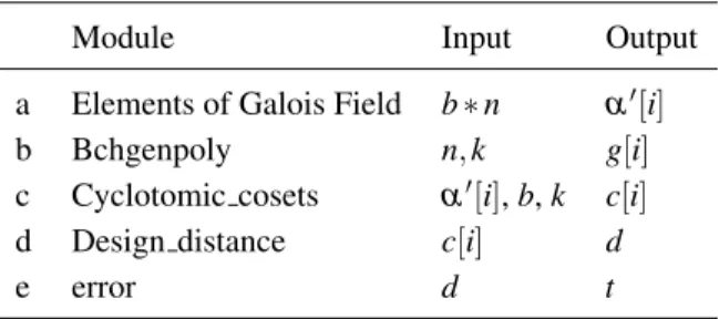
=1 and after we obtain the minimal polynomials of these elements. Finally, we get a non-primitive polynomial with the help of these minimal polynomials. Thus, these design distances are calculated through which the number of errors that can be corrected in each BCH code are determined. Some methods are developed in order to achieve a specified result. In Table 3, we show a list of these methods and its description.

Table 3: Encoding modulation description.

Module Input Output

a Elements of Galois Field b∗n α′[i]

b Bchgenpoly n,k g[i]

c Cyclotomic cosets α′_{[i],b,k c[i]}

d Design distance c[i] d

e error d t

The steps of the algorithm are explained as follows:

a. Elements of Galois field (alpha array)α′[i]).

This step calculates all the elements of the Galois fieldGF(2bn)using a root, sayα′, of a non-primitive polynomial of degreebssuch that(α′₎bn_{=1. The elementα}′_{is called of alpha array}

and denoted byα′[i]. Now, denote the index array byA[index]. For a given inputb∗n, the non-primitive polynomial of degreebs gives the first element of the arrayα′[i]. By increasing its power, each element of the arrayα′_{[i]is calculated in outer loop. Then in nested while loop their}

Algorithm 1:

1 begin

2 INPUTbandn

3 bn←b∗n

4 InitializeA[index]from 1 tobn−1 5 Initializeα′[i]↼0

6 Initialize index↼1 7 WHILE index6=0 8 markA[index]↼0 9 Initializev↼index

10 Calculate next candidate,p_i, byrem(index,bs)

11 α′[i]↼v

12 WHILE current position ofA[index] =0 13 IF current position<A[index]size

14 i+ +

15 ELSEIF

16 i←0

17 BREAK

18 ENDIF

19 ENDWHILE

20 ENDWHILE

21 end

b. BCH generator polynomial(g[i]).

The Matlab builds a function and its complete documentation is found under http://www.mathworks.com/help/comm/ref/bchgenpoly.html. In this module, we get the generator polynomial of primitive BCH code of lengthn.

1 INPUTnandk

2 OUTPUTg[i]

c. Cyclotomic cosets(c[i]).

Givenα′[i], dimension of code kand positive integerb, cyclotomic cosetsc[i] are calculated. Length of c[i] is initialized to at max b∗k, in short all elements should not exceed the max length. Loop start from 2 to max length and calculate unique values in givenα′[i]. The process stops when we get sum of two elements =2. Once cyclotomic cosets are calculated, we can calculate the minimal polynomials for BCH codes.

d. Non-primitive generating polynomialg′[i].

Algorithm 2:

1 begin

2 INPUTα′[i],b,k 3 Initialize cal coset↼0 4 Initialize len cal coset↼0 5 Initialize code length↼b∗k 6 Initialize len coset↼length ofc[i] 7 Initialize code↼b∗k

8 FORi↼2 to len coset 9 cal coset↼c[i]at positioni

10 IFi6=2 THEN

11 code length↼bkcal coset

12 ENDIF

13 PRINTc[i]

14 END FOR

15 end

play an integral role for calculating non-primitive BCH generating polynomial. It is denoted by g′in our algorithm. We are interested in rows of obtained matrix. Using the matrix we obtained, the code for non-primitive generating polynomial of lengthb. Finally these values are printed out and saved in file for further usage.

Algorithm 3:

1 begin

2 INPUTp[i],b

3 Initialize len↼length ofp[i] 4 Initialize size array↼len×b

5 Initializep′[i]of length size array i.e.p′[i]↼0 6 Initialize index↼1

7 Initialize len coef array↼0

8 FORitaking values from 2 to len 9 IFp′[i]ati6=0 THEN

10 Initialize coef array↼b∗(i−1)

11 increment index

12 ENDIF

13 ENDFOR

14 len coef array↼length of coef array 15 FOR jtaking values from 1 to len coef array 16 g′(i)at positionjof coef array↼1

17 ENDFOR

18 g′[i]↼1 top′[i]

19 PRINTg′[i]

e. Designed distance(d).

Here design distance is calculated fromg′[i]. The length of coset arrayclis determined and then iterate index from 2 tocl, calculate next indexniby increment current index. Ifni≤cl, then next element of coset is calculated to the value of coset array at position of next index. Otherwise the bnis assigned to next coset. The whole process iterates to lencoset coset and finally stops at the last coset. Design distancedis calculated from the last value of coset array at position 1.

Algorithm 4:

1 begin

2 INPUTc[i]

3 Initialize lencoset↼cl 4 Initializeni↼0 5 Initialize next coset↼0 6 FOR index from 2 tocl

7 ni↼increment index

8 IFni≤clTHEN

9 next coset↼c[i]at positionni

10 ELSEIF

11 next coset↼bn

12 ENDIF

13 ENDFOR

14 d↼next coset at position 1. 15 end

f. Error correction capability.

For given designed distanced, the error correction capability of a codetis calculated.

Algorithm 5:

1 begin

2 INPUTd.

3 errort↼(d−1)/2. 4 end

3.2 Error correction in received polynomial (decoding)

Table 4: Encoding modulation description.

Module Input Output

a Syndrome Matrix d,bn,bk,α′_{,r[i] S}′_[i]

b CalculateDmatrix t,S′[i] Dmatrix

c IsDinvertible t,Dmatrix |D|6=0

d error locator poly t,Dmatrix,S′[i] f[i]

e error position f[i] e[i]

f error values t,S[i],Dmatrix,e[i],bn,pm[i] ev[i]

h Correct recieved t,bn,e[i],ev[i],r[i],α′ v[i]

polynomial

a.Syndrome matrixS(′[i]).

Given design distanced,bn, message lengthbkand received polynomialr[i], syndrome matrix S′[i]can be calculated. The length ofS′[i]is initialize to the difference ofbnandbk, i.e.,bn−bk. Furthermore,S′[i]is initialized by element of Galois field at positionii.e.GF[i]. Nested loop are used to calculateS′[i]. Upper loop is limited to the length ofbn+d−2, whereS′[i]equalizes to power ofα′_{and in nested loopS}′_{[i]equalize to power ofS}′_{[i]and the iterator. Once the values of}

S′[i]are filled with the above values ofS′[i], it follows that theseS′[i]can be calculated as product ofr[i]and(S′[i])t_.

Algorithm 6:

1 begin

2 INPUTd,bn,bk,α andr[i] 3 Initialize lenSyndrome↼bn−bk 4 InitializeS′[i]↼GF[i]of len Syndrome 5 Initialize valueSynd↼0

6 Initialize valueSynd↼GF[i]lengthbn 7 Initialize loopLimit↼bn+d−2 8 FORi↼bnto loop limit

9 valueSynd↼αi

10 FOR j↼1 tobn

11 evalSynd↼valueSynd powers j

12 ENDFOR

13 S′[i]↼received poly∗transpose of evalSynd

14 ENDFOR

15 PRINTS′[i] 16 end

b.Dmatrix(D[i]).

follows: calculateGF[i]of lengthtandD-matrix is initialized to that value.D[i]in nested loop for loops. Both loops iterates from 1 tot.D[i]values areS′[i]values at positioniof sum of loops iterators to 1.

Algorithm 7:

1 begin

2 INPUTt,S′[i]

3 CalculateGF[i]of lengtht 4 InitializeDmatrix↼GF[i] 5 FOR indexi1 taking from 1 tot 6 FOR indexi2 taking from 1 tot

7 Dmatrix↼S′[i]at positioni1+i2−1

8 ENDFOR

9 ENDFOR

10 end

c. IsDinvertible.

This module check ifD[i]is invertible. IfD[i]is invertible, then the algorithm works, otherwise errortis decremented andDmatrix is again calculated. These operations are carried out till error tbecomes 0. Iftbecomes 0, then algorithm will exit i.e panic condition occurs as in step 10.

Algorithm 8:

1 begin

2 INPUTtandD[i]

3 IFD[i]is invertible THEN 4 continue algo // goto step 5.

5 ELSEIF

6 decrementt;

7 IFtequals 0

8 goto STEP 3

9 ENDIF

10 ENDIF

11 // Panic Condition

12 IFtequals 0

13 Print ERROR cannot be corrected.

14 EXIT algo

15 ENDIF

16 end

d.Error locator polynomial(f[i]).

Given inputt,D[i]andS′[i], error locator polynomial f[i]is calculated. First, initialize product matrixpm[i]and f[i]toα′t_{[i]. Then, iterate the loop from 1 tot,pm[i]is filled with the value of}

T′′[i]. Once the temporary matrixT′′[i]is achievedf[i]is taken as the transpose of that temporary matrix(T′′[i])t _{discuss in step 10.}

Algorithm 9:

1 begin

2 INPUTt,D[i]andS[i] 3 Createα′t[i]

4 Initializepm[i]↼α′t[i]

5 Initialize f[i]↼α′t[i]

6 Initialize temporary matrixT′′[i]of sizet↼0 7 FOR indexitaking values from 1 tot

8 pm[i]↼S[i]at positiont+i

9 ENDFOR

10 T′′[i]↼(S[i])−1∗pm[i] 11 f[i]↼(T′′[i])t

12 f[t+1]↼1 // coefficient of f[t+1] =1 13 end

e. Error position matrix(e[i]).

Based on f[i]we can determine error position. First, the roots of f[i]is calculated and then we take its inverse. The values we obtain are in matrix form and these manifest error position.

Algorithm 10:

1 begin

2 INPUT f[i]

3 Initialize error pos matrixe[i]↼0 4 Initialize root matrix↼0

5 root matrix↼roots of f[i]

6 e[i]↼inverse of roots of f[i] 7 PRINTe[i]

8 end

f. Error values(ev[i]).

Once error positione[i]is determined we can easily calculate their respective values. The nested for loops are used to determine error values. Both of the loops iterate from 1 tot, in the first loop values fromD matrix can be taken while in the next loop value of product matrixpm[i]can be taken along withS′[i]. Finally,ev[i]get equated to(Dmatrix∗pm[i])−1_{as discusses on line 9.}

g. Correct received polynomialr[i].

Once we have calculated error positionse[i]and error valuesev[i]the received polynomialr[i]

Algorithm 11:

1 begin

2 INPUTt,S[i],D[i],e[i],bnandpm[i] 3 Initializeev[i]↼0

4 FOR 1≤i1≤t

5 FOR 1≤i2≤t

6 D[i]ati1 andi2↼e[i]ati2∗(i1+bn−1)

7 ENDFOR

8 pm[i]ati1↼S[i1]

9 ENDFOR

10 ev[i]↼(Dmatrix∗pm[i])−1 11 PRINTev[i]

12 end

Galois field. The received polynomial is corrected by subtracting error polynomial and we get the corrected codewordv[i].

Algorithm 12:

1 begin

2 INPUTt,bn,e[i],ev[i],r[i]andα′ 3 calculateGF[i]of lengthbn. 4 Initialize est error↼GF[i] 5 Initialize est code↼GF[i] 6 Initialize alpha val↼0

7 FOR 1≤i≤t

8 FOR 1≤j≤bn

9 alpha val↼(α′)j−1

10 IF alpha val=elemente[i]atiTHEN

11 est error position j↼est error at position j+ev[i]ati

12 ENDIF

13 ENDFOR

14 est code↼r[i]+est error

15 PRINT est code

16 elements ofpm[i]ati1↼S′[i]elements ati1

17 ENDFOR

18 ev[i]↼Dmatrix∗pm[i] 19 PRINTev[i]

20 end

Example 3.1.For the code of length45simulation is carried out as follows: in this case b=3 and n=15. Using n=15and k=11, Matlab’s build in functiongenpolyis invoked in order to find primitive polynomial, i.e., p(i) =x4+x+1, as explain in Table 3. With b=3and p(i) =

Table 1, is invoked to find the power of alpha tillα45_{=1. With coset array in hand, the designed}

distance d can be calculated, which is the first element of next coset array. Last but not the least error t is calculated against the given designed distance d. Code rate R is also calculated against each k1and bn but is not mentioned in previous section. The output are as follows: Cyclotomic

cosets for(45,33) = [1 2 4 8 16 32 19 38 31 17 34 23], t1=1and R1= (0.73333). Cyclotomic

cosets for(45,29) = [3 6 12 24], t1=2and R1= (0.64444). Cyclotomic cosets for(45,23) = [5

10 20 40 35 25], t1=3and R1= (0.51111). Cyclotomic cosets for(45,11) = [7 14 28 11 22 44 43

41 37 29 13 26], t1=4and R1= (0.24444). Cyclotomic cosets for(45,5) = [15 30], t1=10and

R1= (0.11111). Now comes error correction in received polynomial. In this the code(45,29)is

taken under consideration, with designed distance d1=5and t1=2. Let the received polynomial

be

x44+x16+x13+x12+x11+x7+x3+x+1.

With the given values d1, k1, and received polynomial, syndrome matrix is calculated. The output

for syndromes are S1=α2, S2=α4, S3=α30, S4=α8. Next, we arrange syndrome values

in linear equation form that is Ax=B. Where A= [S1, S2; S2, S3] and B= [S3, S4]. Matrix

A is named as t matrix of t×t dimension. Thus, we find the whether the t matrix is singular or not. If the determinant of t matrix is nonzero then error locator polynomial is calculated. Next error position is calculated from sigma matrix which is obtained from the coefficients of error locator polynomial. For the given values, error positions are44and11. Hence the error polynomial is x44+x11. On subtracting error polynomial from received polynomial the following code polynomial

x16+x13+x12+x7+x3+x+1

is obtained. All of the above equations are obtained by using Matlab symbolic toolbox.

With the help of the above discussed algorithm many examples on non-primitive BCH codes of lengthbn,b2_n,b3_{nare constructed corresponding to primitive BCH code of lengthn. The}

parameters for all binary non-primitive BCH codes of lengthbn,b2n,b3n, wheren≤26−1 and bis either 3 or 7 are given in Table 5.

Table 5 manifests the error and code rate values against some selected codes which we have obtained after simulating our algorithm. These codes are of lengthbn,b2_nandb3_{n, wheren≤}

26−1, andb=3, 7.k1,k2andk3are dimensions of the codesCbn,Cb2_nandC_b3_n, respectively.

Interleaved Codes

From Table 5, it is observed that corresponding to a primitive(n,k) code there are(bn,bk),

Table 5: Parameters of binary non-primitive BCH codes.

n bn k1 t1 R1 b2n k2 t2 R2 b3n k3 t3 R3

15 45 33 1 0.733 135 99 1 0.733 405 297 1 0.733 29 2 0.644 87 2 0.644 261 2 0.644 23 3 0.511 69 3 0.511 207 3 0.511 11 4 0.244 33 4 0.244 99 4 0.244 7 7 0.155 29 7 0.214 87 7 0.214 5 10 0.111 23 10 0.170 69 10 0.170 1 22 0.022 11 13 0.081 33 13 0.081 7 22 0.051 29 22 0.071 5 31 0.037 23 31 0.056 1 67 0.007 11 40 0.027 7 67 0.017 5 94 0.012 1 202 0.002

63 189 171 1 0.904 567 513 1 0.904 1701 1539 1 0.904 165 2 0.873 495 2 0.873 1485 2 0.873 147 3 0.777 441 3 0.777 1323 3 0.777 129 4 0.682 387 4 0.682 1161 4 0.682 123 5 0.650 381 5 0.672 1143 5 0.671 105 6 0.555 327 6 0.576 981 6 0.576 87 7 0.460 273 7 0.481 819 7 0.481 81 10 0.428 255 10 0.449 765 10 0.449

respectively. The code(49,28)is interleaved code of depth 7, which is formed by interleaving the following 7 codewords from(7,4)code that is(0000000),(1101000),(0000000),(0000000),

(0000000),(0000000)and(0000000). on writing them column by column it gives

v1= (01000000100000000000001000000000000000000000000000)∈C49.

In a similar way, codeword of(343,196)and(2401,1372)are obtained by writing column by column 7 codeword ofC49andC343. Therefore, for decoding a received polynomial inC343one

can easily reverse the process and correct errors in the codeword of eitherC49orC7.

ACKNOWLEDMENT

Acknowledgment to FAPESP by financial support 2013/25977-7. The authors would like to thank the anonymous reviewers for their intuitive commentary that signicantly improved the worth of this work.

RESUMO. Neste trabalho, apresentamos um m´etodo que estabelece como uma sequˆencia de c´odigos BCH n˜ao primitivos pode ser obtida atrav´es de um dado c´odigo BCH primitivo. Para isso, utilizamos uma t´ecnica de construc¸˜ao diferente da t´ecnica rotineira de c´odigos BCH e usamos a estrutura de an´eis monoidais em vez de an´eis de polinˆomios. Conse-quentemente, mostramos que existe uma sequˆencia {C_bj_n}1≤j≤m, ondebjn ´e o compri-mento do c´odigoCbj_n, de c´odigos BCH bin´arios n˜ao primitivos em vez de um dado c´odigo

bin´ario BCHCnde comprimenton. Algoritmos simulados via Mathlab para codificac¸˜ao e decodificac¸˜ao para este tipo de c´odigos s˜ao introduzidos. O algoritmo via o Matlab fornece rotinas para a construc¸˜ao de um c´odigo BCH primitivo, mas imp˜oe v´arias restric¸˜oes, como por exemplo, o grausde um polinˆomio irredut´ıvel primitivo deve ser menor que 16. Este trabalho trata-se de polinˆomios n˜ao-primitivos irredut´ıveis com graubs, que s˜ao maiores do que 16.

Palavras-chave: Anel monoidal, c´odigos BCH, polinˆomio primitivo, polinˆomio n˜ao-primitivo.

REFERENCES

[1] A.A. Andrade & P. Jr. Linear codes over finite rings.TEMA – Trends in Applied and Computational Mathematics,6(2) (2005), 207–217.

[2] A.A. Andrade, T. Shah & A. Khan. A note on linear codes over semigroup rings.TEMA – Trends in Applied and Computational Mathematics,12(2) (2011), 79–89.

[3] A.S. Ansari & T. Shah. An association between primitive and non-primitive BCH codes using monoid rings.EURASIP - Journal on Wireless Communications and Networking,38(2016).

[5] A.V. Kelarev. “Ring constructions and applications”. World Scientific Publishing Co. Inc., New York (2002).

[6] A.V. Kelarev & P. Sol´e. Error-correcting codes as ideals in group rings.Contemporary Mathematics, 273(2001), 11–18.

[7] S. Lin & J. D. J. Costello. “Error control coding: fundamentals and applications”. Prentice Hall Professional Technical Reference, New York (1994).

[8] S.R. Nagpaul & S.K. Jain. “Topics in applied abstract algebra”, The Brooks/Cole Series in Advanced Mathematics. New York (2005).

[9] V.S. Pless, W.C. Huffman & R.A. Brualdi. “Handbook of coding theory”. Elsevier, New York (1998).

[10] A. Poli & L. Huguet. “Error-correcting codes: theory and applications”. Prentice-Hall, New York (1992).

[11] T. Shah, Amanullah & A.A. de Andrade. A decoding procedure which improves code rate and error corrections.Journal of Advanced Research in Applied Mathematics,4(4) (2012), 37–50.

[12] T. Shah, Amanullah & A.A. de Andrade. A method for improving the code rate and error correction capability of a cyclic code.Computational and Applied Mathematics,32(2) (2013), 261–274.

[13] T. Shah & A.A. de Andrade. Cyclic codes throughB[X],B[X;_{k p}1Z0]andB[X;_p1kZ0]: a comparison.

Journal of Algebra and its Applications,11(4) (2012), 1250078, 19.

[14] T. Shah & A.A. de Andrade. Cyclic codes through B[X;a_bZ0], with _ba ∈Q+ and b=a+1, and

encoding.Discrete Mathematics, Algorithms and Applications,4(4) (2012), 1250059, 14.

[15] T. Shah, A. Khan & A.A. Andrade. Encoding through generalized polynomial codes. Comp. Appl. Math.,30(2) (2011), 349–366.

[16] T. Shah, M. Khan & A.A. de Andrade. A decoding method of annlength binary BCH code through (n+1)nlength binary cyclic code.Anais da Academia Brasileira de Ciˆencias,85(3) (2013), 863–872.

[17] T. Shah & A. Shaheen. Cyclic codes as ideals inF2[x;aN0]n,F2[x]an, andF2[x;1bN0]abn: a linkage.