Pesq. agropec. bras., Brasília, v.48, n.6, p.589-596, jun. 2013 DOI: 10.1590/S0100-204X2013000600003 Anderson Rodrigo da Silva(1) and Carlos Tadeu dos Santos Dias(1)
(1)Universidade de São Paulo, Escola Superior de Agricultura Luiz de Queiroz, Departamento de Ciências Exatas, Avenida Pádua Dias, 11,
CEP 13418‑900 Piracicaba, SP. E‑mail: ar.silva@usp.br, ctsdias@usp.br
Abstract – The objective of this work was to propose a way of using the Tocher’s method of clustering to obtain a matrix similar to the cophenetic one obtained for hierarchical methods, which would allow the calculation of a cophenetic correlation. To illustrate the obtention of the proposed cophenetic matrix, we used two dissimilarity matrices – one obtained with the generalized squared Mahalanobis distance and the other with the Euclidean distance – between 17 garlic cultivars, based on six morphological characters. Basically, the proposal for obtaining the cophenetic matrix was to use the average distances within and between clusters, after performing the clustering. A function in R language was proposed to compute the cophenetic matrix for Tocher’s method. The empirical distribution of this correlation coefficient was briefly studied. For both dissimilarity measures, the values of cophenetic correlation obtained for the Tocher’s method were higher than those obtained with the hierarchical methods (Ward’s algorithm and average linkage – UPGMA). Comparisons between the clustering made with the agglomerative hierarchical methods and with the Tocher’s method can be performed using a criterion in common: the correlation between matrices of original and cophenetic distances.
Index terms: cluster analysis, optimization methods, clustering consistency.
Um coeficiente de correlação cofenética para o método de Tocher
Resumo – O objetivo deste trabalho foi propor uma forma de uso do método de Tocher para obtenção de uma matriz análoga à matriz cofenética obtida para métodos hierárquicos, o que permitiria o cálculo de uma correlação cofenética. Para ilustrar a obtenção da matriz cofenética proposta, foram utilizadas duas matrizes de dissimilaridade – uma obtida com a distância quadrada generalizada de Mahalanobis e outra com a distância euclidiana – entre dezessete cultivares de alho, com base em seis caracteres morfológicos. Basicamente, a proposta para obtenção da matriz cofenética foi a de usar, após a realização do agrupamento, as distâncias médias intra e intergrupos. Uma função em linguagem R foi proposta para computar a matriz cofenética para o método de Tocher. A distribuição empírica desse coeficiente de correlação foi estudada de forma sucinta. Para as duas medidas de dissimilaridade, os valores do coeficiente de correlação cofenética obtidos para o método de Tocher foram superiores aos obtidos com os métodos hierárquicos (algoritmo de Ward e ligação média – UPGMA). Comparações entre agrupamentos feitos com os métodos hierárquicos aglomerativos e com o método de Tocher podem ser realizadas com o uso de um critério em comum: o da correlação entre matrizes de distâncias cofenéticas e originais.Termos para indexação: análise de agrupamento, métodos de otimização, consistência do agrupamento.
Introduction
Tocher’s optimization method (Rao, 1952) allows establishing mutually exclusive clusters of objects according to an objective function that adopts the criterion of optimization, which minimizes the average distance intra‑cluster and maximizes the average distance inter‑cluster. This method has been used in studies involving quantification of the genetic variability between individuals, both in plants (Gouvêa et al., 2010; Rajamanickam & Rajmohan, 2010; Gorji & Zolnoori, 2011; Leão et al., 2011; Matsuo et al.,
2012) and animals (Barbosa et al., 2005). Descriptions for the clustering process with Tocher’s method can be found in the work of Sharma (2006) and Cruz et al. (2011).
This measure is known as cophenetic correlation coefficient, proposed by Sokal & Rohlf (1962), and it is available in most statistical computer packages. Since then, comparisons between clustering results have been performed with the cophenetic correlation (Kopp et al., 2007; Gonçalves et al., 2008; Cargnelutti Filho et al., 2010; Cargnelutti Filho & Guadagnin, 2011). This is due to the fact that the process of construction of phenograms allows calculating a cophenetic matrix.
However, the Tocher’s method does not involve a construction of a phenogram to perform the clustering. Thus, the clustering consistency has been evaluated indirectly, based on observation of the results of hierarchical clustering and other multivariate methods (Bertan et al., 2006; Leal et al., 2008; Silva, 2012), including ordering techniques which, sometimes, became impractical due to the excessive number of variables and objects. The fact is that the application of some multivariate methods, such as discriminant analysis, requires at least that the classificatory variables are numerical, unlike evaluation by cophenetic correlation, which needs only the clustering result.
Therefore, this work follow the premise of Sneath & Sokal (1973), in which cophenetic values can be obtained even by ordering methods,
The objective of this work was to propose a way of using the Tocher’s method of clustering to obtain a matrix similar to the cophenetic one obtained for hierarchical methods, which would allow the calculation of a cophenetic correlation.
Materials and Methods
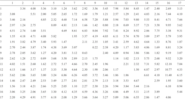
Tocher’s method operates on dissimilarity (or similarity) matrix between individuals. To illustrate the obtaining of the proposed cophenetic matrix, two dissimilarity matrices (Table 1) were used, the first one was obtained by the generalized squared Mahalanobis distance (D2), and the other by the Euclidian distance between 17 garlic cultivars, based on six morphological characters, extracted from Silva (2012).
Tocher’s method was applied based on the referred matrices, and the clustering results of 17 garlic cultivars were used to obtain the cophenetic matrices. The following cluster groups were formed: 1, Mahalanobis distance (cultivars 8, 9, 12, 4, 10, 2, 7, 15) and Euclidean distance (8, 9, 4, 10, 2, 12, 11); 2,
Mahalanobis distance (1, 6, 14) and Euclidean distance (7, 15, 17, 6, 1); 3, Mahalanobis distance (11, 13) and Euclidean distance (3, 5); 4, Mahalanobis distance (3, 5) and Euclidean distance (16); 5, Mahalanobis distance (16) and Euclidean distance (14); and 6, Mahalanobis distance (17) and Euclidean distance (13).
As in the hierarchical methods, the cophenetic matrix consists of the cophenetic distances, i.e., the fusion level of entities; the proposal for Tocher’s method is to get the cophenetic matrix from the average distances within and between clusters.
The average distance within k‑th cluster is obtained by averaging the distances pairs of individuals within cluster, according to the following expression:
-1 n
i=1
k n
j>i j , i k
k
k
k k
2, n j, i , d n (n - 1)
2 d
in which: nk is the number of individuals in the k‑th cluster; and di,j is the distance between the individuals i and j allocated in the k‑th cluster. Obviously, nk = 1 dk = 0.
The average distance between the k‑th and the k'‑th cluster is obtained by averaging the distances between crossed pairs of individuals from two clusters involved, according to the following equation:
k k '
n n
k ,k ' i, j
k k' 1
d d , k k ',
n n
i=1 j=1
in which: nk and nk' are, respectively, the number of individuals in the k‑th and k'‑th clusters; and di,j is the distance between the i‑th individual from the k‑th cluster, and the j‑th individual from the k'‑th cluster. Obviously, nk = nk' = 1 dk,k' = di,j.
Being g the number of clusters formed by Tocher’s method, it can be seen that the actual number of distances involved in the construction of the cophenetic matrix is only a function of the number of formed clusters, expressed by g(g + 1)/2. This fact implies that the calculations involved to obtain that matrix can be similarly extended to the modified Tocher’s method, proposed by Vasconcelos et al. (2007). Therefore, it is noteworthy that the construction of this matrix depends directly on the number of clusters formed by the method.
Pesq. agropec. bras., Brasília, v.48, n.6, p.589‑596, jun. 2013 DOI: 10.1590/S0100‑204X2013000600003 Matrices containing the average distances within
clusters on the main diagonal and average distances between clusters off‑diagonal were constructed to facilitate obtaining the cophenetic matrix.
Based on the relationships observed in Figure 1, the cophenetic matrices were obtained, considering that the phenetic relationship between two cultivars allocated in the same cluster can be represented by the
Table 1. Dissimilarity matrix between 17 garlic cultivars, based on the generalized squared Mahalanobis distance (upper triangular matrix) and the Euclidean distance (lower triangular matrix).
1 2 3 4 5 6 7 8 9 10 11 12 13 14 15 16 17
1 3.34 4.08 5.36 3.10 1.24 3.62 2.92 3.56 5.45 7.98 5.84 8.45 1.47 2.40 2.69 3.13
2 3.08 5.51 2.00 5.05 2.65 1.72 1.69 1.79 1.21 2.57 1.29 2.41 4.03 2.16 7.44 4.10
3 3.46 2.16 4.85 2.32 4.68 7.14 6.58 7.20 5.88 5.94 7.03 9.80 5.53 8.41 4.71 7.66
4 2.97 1.24 2.75 8.09 4.81 2.13 1.66 1.42 0.80 2.18 0.69 3.37 7.21 3.58 9.95 3.62
5 4.51 2.74 1.60 3.51 4.69 8.61 6.83 8.04 7.92 7.41 8.24 8.92 2.86 7.75 3.38 9.31
6 1.55 4.18 4.71 4.08 5.82 1.93 3.37 4.19 4.03 6.11 5.74 8.70 3.09 2.97 5.79 3.95
7 1.91 3.82 4.79 3.40 5.93 1.47 2.11 2.35 1.05 3.41 2.59 4.62 4.64 1.33 8.76 1.87
8 2.70 2.44 3.87 1.74 4.38 3.69 3.07 0.22 2.38 4.20 1.17 3.83 4.86 1.69 8.81 3.24
9 2.78 2.05 3.62 1.27 4.20 3.81 3.12 0.63 2.40 4.89 0.94 3.86 5.86 1.82 9.19 3.07
10 2.62 1.28 2.72 0.89 3.68 3.58 2.89 2.13 1.75 1.14 1.02 2.13 5.75 2.68 9.52 3.20
11 4.02 1.51 2.60 1.62 2.72 5.17 4.66 2.70 2.45 1.96 2.21 2.32 7.31 5.82 12.18 7.04
12 4.13 1.66 3.17 1.37 3.33 5.30 4.64 2.30 1.90 2.06 1.17 1.50 6.87 2.97 10.77 4.33
13 5.62 2.86 3.65 3.00 3.24 6.86 6.26 4.05 3.72 3.46 1.86 1.86 6.61 4.10 11.40 6.15
14 1.46 2.47 2.49 2.53 3.49 2.77 2.81 2.81 2.79 2.13 3.18 3.53 4.67 2.59 1.95 3.60
15 1.56 3.18 4.21 2.66 5.25 2.05 1.10 2.27 2.30 2.26 3.94 3.84 5.44 2.16 6.10 0.94
16 3.06 3.25 2.06 3.65 3.30 4.12 4.35 4.59 4.36 3.26 4.06 4.49 5.11 2.15 3.89 5.44
17 2.20 4.29 4.91 3.77 6.18 2.08 1.29 3.66 3.64 3.27 5.09 5.06 6.55 2.86 1.47 4.06
Figure 1. Clustering diagrams formed by Tocher’s method representing the relationships of average distances within and between the clusters, based on: A, the generalized squared Mahalanobis distance; and B, the Euclidean distance.
A B
5.44 3.56
3.04
3.26 6.59 (1.74)
(2.31)
8.01 7.07
4.15 4.04 (0.00)
3.47 (1.93)
(0.00)
11.78 8.48
4.33
8.81
7.52
(2.32) 5
2
6
1
3 1
2.67
(0.00) 6
1 2
(1.60)
3.44
3.95
2.15
3.89
2.41
6.14 2.98
4.97 5.11
3.24
4.67
2.97
(1.72) (1.67)
(0.00) (0.00)
2.77 5 4
3
# ‑‑‑‑‑‑‑‑‑‑‑‑‑‑‑‑‑‑‑‑‑‑‑‑‑‑‑‑‑‑‑‑‑‑‑‑‑‑‑‑‑‑‑‑‑‑‑‑‑‑‑‑‑‑‑‑‑‑‑‑
# Writing the function
coph.tocher <‑ function(mat.dc, nobj.cluster, id.cluster)
{
rownames(mat.dc) <‑ NULL colnames(mat.dc) <‑ NULL if(!isSymmetric(mat.dc))
stop(“mat.dc must be a symmetric distance matrix!”) if(length(nobj.cluster) != nrow(mat.dc))
stop(“incompatible dimensions!”)
stopifnot(sum(nobj.cluster) == length(id.cluster)) n <‑ length(id.cluster)
nc <‑ length(nobj.cluster) cl <‑ rep(1:nc, nobj.cluster) aux <‑ rbind(id.cluster, cl) coph <‑ matrix(NA, n, n) for(i in 1:n)
{
for(j in i:n) {
if(i != j){
coph[j, i] <‑ mat.dc[aux[2,][aux[1,] == j], aux[2,] [aux[1,] == i]]
} else {coph[j, i] <‑ 0} }
}
return(as.dist(coph)) }
average distance within cluster, and that the phenetic relationship between two cultivars allocated in different clusters can be represented by the average distance between clusters. For example, based on Mahalanobis distance, the cophenetic distance between the cultivars 1 and 6 is simply the average distance within cluster 2, which is d1,6 = 1.93. However, the distance between the cultivars 1 and 5 is the average distance between clusters 2 and 4, which is d1,5 = 4.15.
After constructing the cophenetic matrices, the correlations between the elements from each matrix of original distances with the respective elements from cophenetic matrix were calculated, according to the expression: ,
2 1 1 n n 2 ij 2 1 n-1 i=1 n j>i 2 ij n-1 1 i n i j ij ij coph d d - c c - d d - c c r i=1 j>i , 1 i n i j ij c ) 1 n -( n 2 c , n-1 1 i n i j ij d n-1) ( n 2 d n-1in which: cij and dij are, respectively, the element of the i‑th row and j‑th column of the cophenetic and original distance matrix; and n is the number of individuals (n = 17 in this case).
The Mantel’s randomization test was applied, based on ten thousand permutations of rows and columns of the cophenetic matrix, in order to test the hypothesis of null correlation between the cophenetic matrix and the original distance matrix, and also to allow the visualization of the empirical distribution of this correlation coefficient.
To compare results, clusterings were performed using two hierarchical methods: Ward’s algorithm and average linkage (UPGMA). The cophenetic correlations for these methods were also calculated, as well as the Mantel´s test.
The distance matrices used in this work and the Tocher’s clustering were obtained with the multivariate analysis module of Genes software version 2009.7.0 (Cruz, 2006). After the calculation of distance matrices, the application of hierarchical methods was performed with the hclust() function from “stats” package of R software, and the cophenetic matrices for these methods
were obtained by the cophenetic() function, also from “stats” package; the Mantel´s test was performed with the mantel.rtest() function from “ade4” package (Dray & Dufour, 2007), all packages were from the version 2.15.2 R Core Team (R Foundation for Statistical Computing, Vienna, AT).
Pesq. agropec. bras., Brasília, v.48, n.6, p.589‑596, jun. 2013 DOI: 10.1590/S0100‑204X2013000600003
Results and Discussion
The proposed cophenetic matrices obtained with the also proposed R function is shown in Table 2. It can
# End (Not run)
# ‑‑‑‑‑‑‑‑‑‑‑‑‑‑‑‑‑‑‑‑‑‑‑‑‑‑‑‑‑‑‑‑‑‑‑‑‑‑‑‑‑‑‑‑‑‑‑‑‑‑‑‑‑‑‑‑‑‑‑‑ Description
The function computes the cophenetic distances for a Tocher’s clustering.
Usage
coph.tocher(mat.dc, nobj.cluster, id.cluster) Arguments
mat.dc ‑> matrix of average distances within (diagonal) and between (off‑diagonal) clusters.
nobj.cluster ‑> vector containing the numbers of objects per cluster.
id.cluster ‑> vector (numeric) for identification of objects.
Details
To define id.cluster, the number 1 must be the lowest value and n (the number of objects) the highest. For example, the first 4 numbers (let us say 12, 28, 3 and 15) refer to the objects of the first cluster, the next 2 numbers (let us say 10 and 1) refer to the second cluster, and so on.
Value
An object of class «dist».
# ‑‑‑‑‑‑‑‑‑‑‑‑‑‑‑‑‑‑‑‑‑‑‑‑‑‑‑‑‑‑‑‑‑‑‑‑‑‑‑‑‑‑‑‑‑‑‑‑‑‑‑‑‑‑‑‑‑‑‑‑
Table 2. Matrix of cophenetic distances between 17 garlic cultivars, obtained by the Tocher’s method based on the generalized squared Mahalanobis distance (upper triangular matrix) and Euclidean distance (lower triangular matrix).
1 2 3 4 5 6 7 8 9 10 11 12 13 14 15 16 17
1 4.33 4.15 4.33 4.15 1.93 4.33 4.33 4.33 4.33 7.52 4.33 7.52 1.93 4.33 3.47 3.56
2 3.62 7.07 1.74 7.07 4.33 1.74 1.74 1.74 1.74 3.26 1.74 3.26 4.33 1.74 8.81 3.04
3 4.97 3.24 7.07 2.32 4.15 7.07 7.07 7.07 7.07 8.01 7.07 8.01 4.15 7.07 4.04 8.48
4 3.62 1.72 3.24 7.07 4.33 1.74 1.74 1.74 1.74 3.26 1.74 3.26 4.33 1.74 8.81 3.04
5 4.97 3.24 1.60 3.24 4.15 7.07 7.07 7.07 7.07 8.01 7.07 8.01 4.15 7.07 4.04 8.48
6 1.67 3.62 4.97 3.62 4.97 4.33 4.33 4.33 4.33 7.52 4.33 7.52 1.93 4.33 3.47 3.56
7 1.67 3.62 4.97 1.67 4.97 1.67 1.74 1.74 1.74 3.26 1.74 3.26 4.33 1.74 8.81 3.04
8 3.62 1.72 3.24 1.72 3.24 3.62 3.62 1.74 1.74 3.26 1.74 3.26 4.33 1.74 8.81 3.04
9 3.62 1.72 3.24 1.72 3.24 3.62 3.62 1.72 1.74 3.26 1.74 3.26 4.33 1.74 8.81 3.04
10 3.62 1.72 3.24 1.72 3.24 3.62 3.62 1.72 1.72 3.26 1.74 3.26 4.33 1.74 8.81 3.04
11 3.62 1.72 3.24 1.72 3.24 3.62 3.62 1.72 1.72 1.72 3.26 2.31 7.52 3.26 11.78 6.59
12 3.62 1.72 3.24 1.72 3.24 3.62 3.62 1.72 1.72 1.72 1.72 3.26 4.33 1.74 8.81 3.04
13 6.14 2.97 3.44 2.97 3.44 6.14 6.14 2.97 2.97 2.97 2.97 2.97 7.52 3.26 11.78 6.59
14 2.41 2.77 2.98 2.77 2.41 2.41 2.41 2.77 2.77 2.77 2.77 2.77 4.67 4.33 3.47 3.56
15 1.67 3.62 4.97 3.62 4.97 1.67 1.67 3.62 3.62 3.62 3.62 3.62 6.14 2.41 8.81 3.04
16 3.89 3.95 2.67 3.95 2.67 3.89 3.89 3.95 3.95 3.95 3.95 3.95 5.11 2.15 3.89 5.44
17 1.67 3.62 4.97 3.62 4.97 1.67 1.67 3.62 3.62 3.62 3.62 3.62 6.14 2.41 1.67 3.89
be seen that, with Mahalanobis distance, the minimum distance between two cultivars in the corresponding cophenetic matrix was 1.74, which equals the distance within cluster 1. Thus, that is the distance between any two cultivars allocated in cluster 1. The greatest distance (11.78) corresponded to the average distance between clusters 3 and 5. In the obtained cophenetic matrix based on clustering with the Euclidean distance, the shortest distance between two cultivars was 1.60 (cultivars 3 and 5), corresponding to the average distance within cluster 3. The greatest distance (6.14) corresponded to the average distance between clusters 2 and 6.
It is important to note that 136 measures of distance were provided by the matrix of the original distances. The construction of each proposed cophenetic matrix involved, actually, 21 measures of distance: 6 within and 15 between clusters. This number is higher than the one of fusion levels obtained with the hierarchical methods, which was 16 for both.
Figure 2. Shepard diagram for association between original and cophenetic distances based on: A, the generalized squared Mahalanobis distance; and B, the Euclidean distance.
Figure 3. Kernel density of cophenetic correlation based on ten thousand permutations, obtained with: A, the generalized squared Mahalanobis distance; and B, the Euclidean distance.
The cophenetic correlation coefficient was calculated on each of the ten thousand permutations performed in the cophenetic matrices obtained with each of the
0 2 4 6 8 10 12
2 4 6 8 10 12
Tocher
0 2 4 6 8 10 12
0 5 10 15 20 25
Ward
0 2 4 6 8 10 12
0 1 2 3 4 5 6
Average linkage
1 2 3 4 5 6 7
2 3 4 5 6
Original distances
1 2 3 4 5 6 7
2 4 6 8 10 12
Original distances
1 2 3 4 5 6 7
1.0 1.5 2.0 2.5 3.0 3.5 4.0
Original distances B
A
Cophenetic distances
Cophenetic distances
-0.5 0.0 0.5 1.0
0.0 0.5 1.0 1.5 2.0 2.5 3.0
Tocher
r = 0.90
-0.5 0.0 0.5 1.0
0 1 2 3 4 5 6
Ward
r = 0.59
-0.5 0.0 0.5 1.0
0 1 2 3 4
Average linkage
r = 0.73
-0.5 0.0 0.5 1.0
0 1 2 3
Cophenetic correlation r = 0.85
-0.5 0.0 0.5 1.0
0 1 2 3 4
Cophenetic correlation r = 0.63
-0.5 0.0 0.5 1.0
0 1 2 3 4
Cophenetic correlation r = 0.71 A
B
Density
Density
Pesq. agropec. bras., Brasília, v.48, n.6, p.589‑596, jun. 2013 DOI: 10.1590/S0100‑204X2013000600003 using Mahalanobis distance, and 0.85 using Euclidean
distance – were even higher than those obtained by the average linkage method – 0.73 using Mahalanobis distance, and 0.71 using Euclidean distance –, which should be the most successful method in maximizing the cophenetic correlation, among hierarchical ones, according to empirical results reported by Sokal & Rohlf (1962) and confirmed by Farris (1969). In a study on the consistency of the clustering pattern of bean with different combinations of dissimilarity measures and clustering methods, Cargnelutti Filho et al. (2010) concluded that the average linkage based on the Euclidean distance actually had the highest cophenetic correlation.
In fact, once the cophenetic matrices for Tocher’s clustering were based on more distances (21) than those obtained by the hierarchical methods (16), it was expected that the representation of the original distance would be more accurate for Tocher’s clustering, for both measures of distance used.
The lowest correlation was obtained by the Ward’s algorithm (0.59) based on Mahalanobis distance. Nevertheless, all correlation values were significant (p<0.001) by Mantel test, indicating the rejection of null hypothesis (null correlation).
With both Mahalanobis distance and Euclidean distance, the empirical distribution of cophenetic correlation coefficient for Tocher’s method was quite similar to those obtained with the hierarchical methods, therefore having comparable quantiles (Figure 3). This means that the proposed cophenetic correlation might be considered a random variable descending from the same population of the cophenetic correlations obtained with the hierarchical methods, and it might serve the same purpose.
In each of the cases showed on Figure 3, an almost symmetric distribution around zero was observed. Regarding this finding, Bryant (1960) stated that, when the actual correlation is null, the distribution of sample correlation coefficient is symmetric around zero, although not exactly Gaussian.
Conclusions
1. The construction of the proposed cophenetic matrix for Tocher’s method depends only on the calculation of average distances within and between clusters.
2. With both the generalized squared Mahalanobis distance and the Euclidean distance, the values
of cophenetic correlation coefficient obtained for Tocher’s method are higher than those obtained with the hierarchical methods (average linkage and Ward’s algorithm).
3. Comparisons between clustering made with agglomerative hierarchical methods and Tocher’s method can be performed using a criterion in common: the correlation between matrices of original and cophenetic distances.
Acknowledgements
To Coordenação de Aperfeiçoamento de Pessoal de Nível Superior (Capes), for the scholarship grant and to Conselho Nacional de Desenvolvimento Científico e Tecnológico (CNPq), for the research grant.
References
BARBOSA L.; REGAZZI, A.J.; LOPES, P.S.; BREDA, F.C.; SARMENTO, J.L.R.; TORRES, R.A.; TORRES FILHO, R.A.
Evaluation of genetic divergence among lines of laying hens using cluster analysis. Revista Brasileira de Ciência Avícola, v.7, p.79‑84, 2005. DOI: 10.1590/S1516‑635X2005000200003.
BERTAN, I.; CARVALHO, F.I.F. de; OLIVEIRA, A.C. de;
VIEIRA, E.A.; HARTWIG, I.; SILVA, J.A.G. da; SHIMIDT, D.A.M.; VALÉRIO, I.P.; BUSATO, C.C.; RIBEIRO, G. Comparação de métodos de agrupamento na representação da distância morfológica entre genótipos de trigo. Revista Brasileira de Agrociência, v.12, p.279‑286, 2006.
BRYANT, E.C. Statistical analysis. New York: McGraw‑Hill, 1960. 303p.
CARGNELUTTI FILHO, A.; GUADAGNIN, J.P. Consistência do
padrão de agrupamento de cultivares de milho. Ciência Rural, v.41, p.1503‑1508, 2011. DOI: 10.1590/S0103‑84782011005000116.
CARGNELUTTI FILHO, A.; RIBEIRO, N.D.; BURIN, C.
Consistência do padrão de agrupamento de cultivares de feijão conforme medidas de dissimilaridade e métodos de agrupamento.
Pesquisa Agropecuária Brasileira, v.45, p.236‑243, 2010. DOI: 10.1590/S0100‑204X2010000300002.
CRUZ, C.D. Programa Genes: biometria. Viçosa: Ed. UFV, 2006.
382p.
CRUZ, C.D.; FERREIRA, F.M.; PESSONI, L.A. Biometria aplicada ao estudo da diversidade genética. Visconde do Rio Branco: Suprema, 2011. 620p.
DRAY, S.; DUFOUR, A.‑B. The ade4 package: implementing the
duality diagram for ecologists. Journal of Statistical Software, v.22, p.1‑20, 2007.
FARRIS, J.S. On the cophenetic correlation coefficient. Systematic Biology, v.18, p.279‑285, 1969.
Genetics and Molecular Research, v.7, p.1289‑1297, 2008. DOI: 10.4238/vol7‑4gmr526.
GORJI, A.H.; ZOLNOORI, M. Genetic diversity in hexaploid wheat genotypes using microsatellite markers. Asian Journal of Biotechnology, v.3, p.368‑377, 2011. DOI: 10.3923/ ajbkr.2011.368.377.
GOUVÊA, L.R.L.; RUBIANO, L.B.; CHIORATTO, A.F.;
ZUCCHI, M.I.; GONÇALVES, P. de S. Genetic divergence of rubber tree estimated by multivariate techniques and microsatellite markers. Genetics and Molecular Biology, v.33, p.308‑318, 2010. DOI: 10.1590/S1415‑47572010005000039.
KOPP, M.M.; SOUZA, V.Q. de; COIMBRA, J.L.M.; LUZ, V.K. da; MARINI, N.; OLIVEIRA, A.C. de. Melhoria da correlação cofenética pela exclusão de unidades experimentais na construção de dendrogramas. Revista da FZVA, v.14, p.46‑53, 2007.
LEAL, J.B.; SANTOS, L.M. dos; SANTOS, C.A.P. dos; PIRES, L.P.; AHNERT, D.; CORRÊA, R.X. Diversidade genética entre acessos de cacau de fazendas e de banco de germoplasma na Bahia. Pesquisa Agropecuária Brasileira, v.43, p.851‑858, 2008. DOI: 10.1590/S0100‑204X2008000700009.
LEÃO, P.C. de S.; MOTOIKE, S.Y. Genetic diversity in table grapes based on RAPD and microsatellite markers. Pesquisa Agropecuária Brasileira, v.46, p.1035‑1044, 2011. DOI: 10.1590/ S0100‑204X2011000900010.
MATSUO, E.; SEDIYAMA, T.; OLIVEIRA, R.D. de L.; CRUZ, C.D.; OLIVEIRA, R.C.T. Characterization of type and
genetic diversity among soybean cyst nematode differentiators.
Scientia Agricola, v.69, p.147‑151, 2012. DOI: 10.1590/ S0103‑90162012000200010.
RAJAMANICKAM, C.; RAJMOHAN, K. Genetic diversity in banana (Musa spp.). Madras Agricultural Journal, v.97, p.106‑109, 2010.
RAO, R.C. Advanced statistical methods in biometric research. New York: J. Wiley, 1952. 390p.
SHARMA, J.R. Statistical and biometrical techniques in plant breeding. Delhi: New Age International, 2006. 432p.
SILVA, A.R. Métodos de agrupamento: avaliação e aplicação ao estudo de divergência genética em acessos de alho. 2012.
67p. Dissertação (Mestrado) – Universidade Federal de Viçosa,
Viçosa.
SNEATH, P.H.A.; SOKAL, R.R. Numerical taxonomy: the
principles and practice of numerical classification. San Francisco: W.H. Freeman, 1973. 573p.
SOKAL, R.R.; ROHLF, F.J. The comparison of dendrograms
by objective methods. Taxon, v.11, p.33‑40, 1962. DOI: 10.2307/1217208.
VASCONCELOS, E.S. de; CRUZ, C.D.; BHERING, L.L.;
RESENDE JÚNIOR, M.F.R. Método alternativo para
análise de agrupamento. Pesquisa Agropecuária Brasileira, v.42, p.1421‑1428, 2007. DOI: 10.1590/ S0100‑204X2007001000008.