Mission Planner for Solar Powered Unmanned Aerial Vehicles

(1)

UNIVERSIDADE DA BEIRA INTERIOR

Engenharia

Mission Planner for Solar Powered Unmanned

Aerial Vehicles

(Versão corrigida após defesa)

Luís Miguel Marques Coelho

Dissertação para obtenção do Grau de Mestre em

Engenharia Aeronáutica

(Ciclo de Estudos Integrado)

Orientador: Professor Doutor Pedro Viera Gamboa

(2)

(3)

Acknowledgments

After living these wonderful student years I have all the pride to say I have the best mother in the world, and I thank her for having worked so hard these years, so I can feel this immense happiness and pride in myself.

I also thank my advisor, Professor Pedro Vieira Gamboa, for all the patience and help during this dissertation.

And finally, I thank my girlfriend and all my friends who gave me motivation and focus to finish and deliver an honest work to be proud of.

(4)

(5)

(6)

(7)

Resumo

Os veículos aéreos não tripulados (UAV’s), inicialmente utilizados para aplicações militares, tornaram-se cada vez mais atraentes para fins civis. A utilização deste tipo de aeronave tem crescido exponencialmente nos últimos anos, tanto para fins profissionais como recreativos, de-vido às inúmeras vantagens que apresentam. Este aumento da procura levou a um crescente investimento no setor, nomeadamente nos UAVs movidos a energia solar, que hoje em dia já ocupam uma pequena fatia do mercado. No entanto, com o aparecimento deste tipo de UAV’s, os softwares de planeamento de missões precisam de ser atualizados de forma a terem em conta a energia fornecida pelo sol. Desta forma, o presente trabalho descreve o desenvolvimento e validação de um planeador de missões para UAV’s movidos a energia solar, capaz de planear e otimizar uma missão, considerando uma estimativa inicial dos parâmetros de cada waypoint (latitude, longitude, altitude e velocidade), e ainda considerando dados reais de previsão me-teorologica e elevação de terreno. Para isso, o planeador de missões considera vários modelos matemáticos, necessários para o cálculo do desempenho da missão, e um algoritmo quadrático sequencial de forma a otimizar a missão inicial. Depois de descrever os modelos teóricos, uma aplicação prática do planeador de missão é feita com o objetivo de verificar o seu desempenho. Em relação à validação, vários resultados divididos por tópicos de interesse são apresentados e discutidos, concluindo: é eficiente em relação ao planeamento de missões, ainda assim, tendo alguns aspetos a serem melhorados.

Palavras-chave

(8)

(9)

Abstract

Unmanned aerial vehicles (UAV’s), initially used for military applications, have become increas-ingly attractive for civilian purposes. The use of this type of aircraft has grown exponentially in recent years, both for professional and recreational purposes, due to the numerous advan-tages they present. The increasingly demand of UAV led to an increase in investment, namely in the development of solar powered UAVs. Nowadays, with the arising of this type of UAV’s, the mission planners have to start to be updated with new features considering UAV’s with pho-tovoltaic solar panels. This way, the present work describes the development and validation of a mission planner for solar powered UAV’s, capable of planning and optimizing a mission given a initial guess of waypoints parameters (latitude, longitude, altitude and airspeed), consider-ing real weather forecast and terrain elevation data. For this, the mission planner considers several mathematical models, required for the calculation of the mission performance, and a sequential quadratic programming algorithm to optimize the initial mission. After it describes the theoretical models, a practical application of the mission planner is done in order to ver-ify its performance. Regarding its validation, several results divided by topics of interest are presented and discussed, concluding that the mission planner works efficiently, regarding the mission planning, even though, it has some aspects to be improved.

Keywords

(10)

(11)

List of Figures

1.1 Example of a mission planning problem solution. . . 1

2.1 Trajectory calculated with a Voronoi method. . . 3

2.2 Example of a graph with the nodes that can be visited and each cost on the segments. 4 2.3 Example of a potential field based algorithm paths. . . 4

2.4 Mission Planner ground station interface example. . . 8

2.5 QBase Mission Planner Interface . . . 9

2.6 QBase Mission Planner Mission . . . 9

3.1 Individual models used for the mission planning . . . 11

3.2 Initial 5 waypoints trajectory example. . . 12

3.3 Flight Path Direction Scheme . . . 14

3.4 2D Interpolation Data . . . 22

3.5 Illustration of the sun’s position. . . 26

3.6 Illustration of the problem. . . 26

3.7 Systems Power distribution. . . 27

3.8 Pseudocode for the management of the electrical Systems. . . 28

3.9 Iterative process flowchart. . . 28

3.10 Simplified scheme of the forward finite differences method used to estimate the gradient at point x. . . . 29

3.11 Sequential Quadratic Programming (SQP) optimization procedure. . . 30

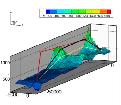
4.1 3D View of the output mission -the black trajectory refers to test pre 1 and the yellow trajectory refers to test pre 2. . . 36

4.2 YZ View of the output mission - Test pre 1 . . . 36

4.3 XY View of the output mission - Test pre 1 . . . 37

4.4 Objective Function Convergence - Test pre 2 . . . 37

4.5 Objective Function Gradients - Test pre 2 . . . 39

4.6 Comparison between test TA 1 and test TA 2. . . 40

4.7 Test’s TA 1 and TA 2 Objective functions convergence. . . 41

4.8 Comparison between the four tests . . . 42

4.9 Comparison between test NU 1 and test NU 2. . . 45

4.10 Comparison between test NU 1 and test NU 2. . . 45

4.11 3D view Real Weather Forecast Data Test RW 1. . . 48

4.12 Comparison between test RW 1 and test RW 2. . . 48

4.13 Comparison between test RW 3 and test RW 4. . . 49

(14)

(15)

List of Tables

3.1 The constant values used in Eqs. above. . . 25

4.1 Code to name the tests. . . 33

4.2 LEEUAV Input Specifications . . . 34

4.3 LEEUAV Motor Specifications . . . 34

4.4 LEEUAV Battery Specifications . . . 34

4.5 LEEUAV Propeller Specifications . . . 34

4.6 Preliminary Tests design variables . . . 35

4.7 Fixed data for Mission planning - Test pre 1. . . 35

4.8 Output Design Variables - test pre 1 . . . 37

4.9 Fixed data for Mission planning - test pre 2. . . 38

4.10 Output Design Variables - test pre 2 . . . 38

4.11 Mission Design Variables Input - Solar Model Behaviour . . . 41

4.12 Mission Fixed Data Input - Solar Model Behaviour . . . 41

4.13 Mission Planner Results - Solar Model Behaviour . . . 42

4.14 Mission Planner Airspeed Results - Solar Model Behaviour . . . 42

4.15 Mission Design Variables Input - Non Uniform Cloud Cover . . . 43

4.16 Mission Planner General Results - Non Uniform Cloud Cover . . . 44

4.17 Output airspeed by segment, cloud cover and solar power by segment - Test NU 1 44 4.18 Output airspeed by segment, cloud cover and solar power by segment - Test NU 2 44 4.19 Mission Design Variables Input - Real Weather Forecast Data . . . 46

4.19 Mission Design Variables Input - Real Weather Forecast Data . . . 47

4.20 Mission Planner General Results - Winter . . . 47

4.21 Output airspeed by segment - RW 1 and 2 . . . 47

4.22 Mission Planner General Results - Summer . . . 48

4.23 Output airspeed by segment - RW 3 and 4 . . . 49

4.24 Mission Design Variables Input - Mission Across Portugal . . . 50

4.25 Mission Planner General Results - Mission Across Portugal . . . 50

(16)

(17)

Acronyms List

AGI Analytical Graphics inc API Application Program Interface ASL Autonomous System Lab ENU East North Up

ERAST Environmental Research Aircraft Sensor Technology ESC Electronical Speed Controller

FFSQP FORTRAN Feasible Sequential Quadratic Programming GBAD Ground Based Air Defence

LEEUAV Long Endurance Electric Unmanned Aerial Vehicle MPT Mission Planning Tools

NASA National Aeronautics and Space Administration PV Photovoltaic

RRT Rapidly-exploring Random Tree SQP Sequential Quadratic Programming UAV Unmanned Aerial Vehicle

(18)

(19)

Nomenclature

a Acceleration [m/s2_]

AZ Sun’s azimuth [deg.]

AZS Photovoltaic panel’s azimuth [deg.]

A, B, C, D, E Coefficient vectors

Bref Energy left constraint reference value

Cc Cloud cover [Oktas]

CD Drag coefficient

CL Lift coefficient

CLmax Maximum Lift coefficient

CLT O Take-off Lift coefficient

Cp Power coefficient

Cp0 Power coefficient at null advance ratio

D Drag Force [N ]

d Propeller diameter [m]

dg Ground distance [m]

dh Height variation [m]

dn Day of the year

dv Design variables

E Mission’s consumed Energy [J ]

Elef t Energy left in the battery

Esolar|pred Predicted Solar energy collected with horizontal photovoltaic panels

[J ]

Esolar_{|T otal} Total Solar energy collected with tilted photovoltaic panels [J ]

F Rolling friction force [N ]

g Gravity acceleration [m/s2_]

H Hour angle [deg.]

h Altitude of flight [m]

hp Actual flight height [m]

href Minimum height constraint reference value [m]

i Current value at each waypoint

I Electric current [A]

Ief f Effective current [A]

Imax Maximum electric current [A]

I0 No load current [A]

j Current value at each segment

J Solar irradiation [W/m2_]

Jcloud Solar power collected considering the cloud cover [W/m2]

J0n Intensity of the extraterrestrial normal solar irradiation [W/m2]

Jmax Propeller maximum advance ratio

JSC extraterrestrial normal solar irradiation constant [W/m2]

JT S Solar power in a tilted photovoltaic panel [W/m2]

(20)

Kt Motor torque constant

Kv Motor speed Constant

L Lift force [N ]

M Mass [kg]

N Propeller speed [rpm]

n Load factor

p Propeller pitch [m]

Pbat Battery power [W ]

Pef f Effective power [W ]

Pele Electric power [W ]

Pmotor Motor power [W ]

Preq Required power [W ]

Pshaf t Motor power at the shaft [W ]

Psolar Solar power [W ]

Psys Systems power [W ]

PT Total electric power [W ]

Q Coordinates of the elevation map’s diagonal [deg.]

Qelevation Elevation data [m]

QIF Inertial Force [N ]

Qm Available torque at the shaft [N m]

Qweather Weather data

R Electric resistance [Ω]

RESC Motor speed controller resistance [Ω]

RU Battery resistance [Ω]

RC Rate of climb [m/s]

res Sun-Earth distance [km]

res,0 Mean Sun-Earth distance [km]

S Wing area [m2_]

SP V Photovoltaic panels area [m2]

T Thrust [N ]

t Time [s]

U Input Voltage [V ]

Uef f Effective voltage [V ]

v True anomaly [deg.]

V Aircraft airspeed [m/s]

Va Average airspeed [m/s]

Vave Average squared airspeed [m2/s2]

Vg Ground speed [m/s]

Vga Average ground speed [m/s]

Vsaf ety Safety speed factor

Vstall Stall speed [m/s]

Vw Wind speed [m/s]

Vwa Average wind speed [m/s]

w Waypoint number

(21)

Greek Letters

α Angle of the photovoltaic panel with the horizontal [deg.]

β Angle of the photovoltaic panel with the normal to the centre of the Earth [deg.]

γa Air path angle [deg.]

γg Angle of trajectory relative to ground [deg.]

δs Solar declination angle [deg.]

δset Motor power setting

δref Maximum motor setting constraint reference value

ε Eccentricity ratio of earth

ζ Zenith angle [deg.]

ηgearbox Gear box efficiency

ηmax Maximum propeller efficiency

ηmotor Motor efficiency

ηp Propeller efficiency

ηP V Photovoltaic panels efficiency

θg Angle of trajectory projection on xy-plane relative to x-axis [deg.]

θi Angle of incidence of the Sun [deg.]

θg Angle of incidence of the wind [deg.]

λ Longitude [deg.]

µ Coefficient of static friction

ρ Air’s relative density [kg/m3_]

τ Transmittance factor

ϕ Latitude [deg.] Ω Motor speed [rpm]

(22)

(23)

Chapter 1

Introduction

This chapter, first introduces the mission planning by a general aproach, followed by the moti-vation and the objectives of this work. The goal of this chapter is to help the reader become familiar with the mission planning concept and understand why and for what purposes this work was done.

1.1 Mission Planning Approach

With all the evolution in aerial vehicles, an entire range of practical problems appeared to be solved. One of those problems was the mission planning problem. Since aircraft routes and flight frequencies are essential for making airline timetables, it is important to plan them ef-fectively in order to achieve a profitable timetable [1].

The mission planning, or path planning problem, has long been seen as one of the fundamental problems in aviation. Originally arising from the need of pre-defined path for each aircraft to follow and so prevent saturated air traffic and mid-air collisions. It is the process of producing a flight plan to describe a proposed aircraft flight between a starting and an ending point. It involves several aspects: fuel calculation, to ensure that the aircraft is able to reach the desti-nation, the aircraft control limitations to secure that the vehicle can do the maneuvers to avoid obstacles, and terrain data to know if there is any possible obstacle to avoid [2].

(24)

1.2 Motivation

The first applications of unmanned aerial vehicles (UAV’s) were military-type. In spite of that, their reducing costs and their increasing capacity made them attractive for civilian applica-tions. Nowadays, the mission planning has become even more important with the increased use of UAV’s. In surveillance missions, for example, UAV’s need a predefined plan of an optimal route with obstacle avoidance and target reaching.

New assigned tasks to UAV’s are demanding better management of energy, in order to reach specific objectives without compromising safety. Therefore, a mission planner that optimizes mission parameters like energy or time can be very useful while setting up the vehicle for op-timal performance. In addition, aircraft performance optimization and flight tests may prove themselves very difficult to do without a previous mission plan. In autonomous flights, if a pro-totype is tested without a mission plan in unknown environments, there is the risk of a crash and, in that case, all the work is lost. In order to avoid that, many mission planning software were created. Yet for non-profit institutions like universities, those software may prove too expensive for the institution to afford it.

In the Department of Aerospace Sciences of the University of Beira Interior there is the Long Endurance Electric UAV (LEEUAV). As it’s name suggests, this UAV was built to do long endurance missions, also, it is a solar powered UAV. So, the main reason for the development of the present thesis is to plan viable missions assuring the safety and the success of its flight.

1.3 Objectives

The main objective of this thesis is to develop and validate a mission planner for solar powered UAV’s. To achieve this objective, a detailed description of the various tasks is shown below:

• Identification of the parameters that feed the mathematical models;

• Development and implementation of a mission performance model required to estimate all the necessary parameters to define a mission;

• Selection of databases that provide real weather forecast and terrain elevation data; • Development and implementation of models that request and return, from the selected

databases, the required data for the mission performance model; • Implementation of a propulsion performance model;

• Implementation of a solar model required to estimate the total energy harvested from the photovoltaic cells;

• Development of the flight energy management algorithm required to estimate the to-tal/partial energy, as well the rates of change;

• Selection and implementation of an algorithm that can solve the mission planning problem; • Verification of the mission planner.

(25)

Chapter 2

State of Art

This chapter first gives an overview of common approaches taken to solve the mission planning problem, then a brief introduction to the solar-powered aircraft is given as well as an historic contextualization of the field of study. Finally, the chapter ends with the presentation of prac-tical applications of different planning tools.

2.1 Methods and Algorithms

To solve the path planning problem it is necessary to research methods and modern computer technology. There are currently five types of methods that can be used to solve this problem [4] [5]

2.1.1 Roadmap-based Method

A roadmap-based method consists in constructing a map that represents the environment space constraints, and then using a search algorithm to find the shortest path [6]. One example of this type of methods is the Voronoi Map method, example in Figure 2.1 . As its name would suggest, it is based on Voronoi diagrams which are used to extract the network representation of the environment. After that, as mentioned above, a search algorithm is used to go through the map analysing the possibilities and, by these means finding the best path.

Figure 2.1: Trajectory calculated with a Voronoi method. [6]

2.1.2 Heuristic Search Algorithm

This type of methods, e.g. Dijkstra’s algorithm, involves knowing some special information about the domain of the problem, so that it is possible to evaluate the heuristic cost of each solution by an heuristic function. It constructs nonoverlapping regions that cover free space and encode cell connectivity in a graph [7]. Dijkstra’s algorithm is used to find the shortest path between two points, it picks the unvisited node with the lowest distance, calculates the distance through it to each unvisited neighbor, and updates the neighbor’s distance if it is smaller. In Figure 2.2 an example of a cell connectivity and the cost of each path is represented.

(26)

Figure 2.2: Example of a graph with the nodes that can be visited and each cost on the segments. [8]

2.1.3 Stochastic Programming Methods

Many Stochastic Programming approaches are based on random sampling, which has a component of probability, e.g. rapidly-exploring random tree (RRT). This algorithm provides a way to search high-dimensional spaces efficiently. It consists of a tree data-structure of samples in the space, created by an algorithm in a way that provides good coverage. The tree-construction algorithm consists in a loop of the following operations: firstly, RRT picks a random sample in the search space, secondly, finds the nearest neighbor of that sample, thirdly, selects an action from the neighbor that heads towards the random sample, then, creates a new sample based on the outcome of the action applied to the neighbor and lastly, adds the new sample to the tree, connecting it to the neighbour. In addition, RRT is biased to grow towards large unsearched areas of the problem [9].

2.1.4 Potential Field-based Methods

Potential field methods are based on the concept of electrical charges. If we see an UAV as an electrically-charged particle Figure 2.3, then obstacles should have the same type of electrical charge in a way to repulse the UAV. Following this group of methods the stream function is constantly used to path finding and obstacle avoidance.

(27)

2.1.5 Optimization algorithm Methods

Optimization algorithms help to minimize or maximize an objective function ,f (x), which is a mathematical function dependent on the Model’s internal parameters. They are used in comput-ing the target design variables ,x, takcomput-ing into account the constraints functions, g(x), defined in the model. An optimization problem can be represented in the following way:

• Given a function f : A→ R

• Sought an element x0∈ A such that f(x0)≤ f(x) for all x ∈ A (minimization) or such that

f (x0)≥ f(x) for all x ∈ A (maximization)

Many real-world and theoretical problems may be modelled in this general framework. Typically,

Ais some subset of the Euclidean spaceRn_{, often specified by a set of constraints, equalities or}

inequalities that the members of A have to satisfy. The domain A of f is called the search space or the choice set, while the elements of A are called candidate solutions or feasible solutions. A local minimum is at least as good as any nearby elements, and a global minimum is at least as good as every feasible element [10]. Generally, unless the objective function is convex in a minimization problem, there may be several local minima. In a convex problem, if there is a local minimum that is interior (not on the edge of the set of feasible elements), it is also the global minimum, but a non-convex problem may have more than one local minimum not all of which need to be global minima [10].

2.1.6 Methods Comparison

These different methods are normally combined to use their best capabilities in order to bet-ter solve the path planning problem. The roadmap-based method is usually used to extract a network representation of the environment. This helps to stablish the space boundaries of the path, yet it needs a search algorithm to evaluate and optimize each path. On the other hand, heuristic search algorithms need a previously defined space with the heuristic cost of each seg-ment of the map pre-defined. Therefore, sampling-based can also serve as a search algorithm, being faster than the heuristic search algorithms as it does not need to visit each path to find a solution, yet that solution may not be the global solution as it works by randomly exploring the space. The potential field based methods have a great behaviour in respect to obstacle avoid-ance, even though the path is limited to the defined stream functions. Finally, optimization algorithm can be used to solve any problem, if it is expressed as a mathematical function, as well as, optimize more than one function, yet, it may not find the global solution and find only a local solution like the sampling based methods.

2.2 Brief History of Electrical and Solar Powered Flight

Since 1884, when a couple of French army officers named Renard and Krebs used a hydrogen-filled dirigible powered by batteries and won a 10 km race around Villacoulbay and Medon, the electrical aerial vehicles became a possibility for the researchers [11]. In spite of the this suc-cess for the electrical motors, after the arrival of the piston engines this clean energy motors were abandoned almost for a century [11][13]. Nevertheless, a first step towards solar powered flight had been taken.

(28)

In the 1960s Fred Militky of Kerkheim Tech begun to work with lightweight free flight mod-els powered by toy motors and one shot saline batteries. Although these modmod-els have flown, they were considered unsuccessful. Later in 1970 Roland and Robert Boucher started their ex-periments with electrical flight [12]. At this point, the combination of electrical flight and solar cells was made for the first time. Robert Boucher built a couple of pilotless solar-powered air-craft under contracts with the Defence Advanced Research Projects Agency [11].

In Germany, there was another solar model airplane project in work, which was under the responsibility of Helmut Bruss. Yet this model could not achieve level flight due to the over heating of its solar cells [12]. One year later, his friend Fred Militky, achieve the first flight totally powered by solar energy, with Solaris. This flight was made on the 16th of August 1976, when it reach 50m of altitude by making three flights by 150 seconds each[12].

Nowadays, aircraft internal combustion engines have a much higher endurance than electri-cal motors. The problem is not the high energy required by the electrielectri-cal flight, is because it results in an increase of weight and space. The combination of electric flight and solar cells has become very useful since the batteries size and weight can be reduced, thus allowing long endurance flights.

This reintegration of electrical powered flight, led to an investment in many researches and experiments in electrical aircraft, trying to achieve better results, namely in the efficiency and endurance field [13].

2.2.1 Evolution of Solar Powered Aircraft

The evolution in the electrical flight field made possible to the pioneers to start experiments for the solar powered flight. The first solar powered aircraft, a radio controlled model plane called Sunrise I, was develop by Roland Boucher and made its first flight in 4th of November of 1974 in California [14]. Four years later, on 19 December 1978, Solar One, a manned solar-powered aircraft developed by Britons David Williams and Fred To, achieved its first flight at Lasham Airfield, Hampshire. This conventional shoulder wing monoplane was build in the first place to be human powered. However, it was proved too heavy to be so. Thus, that is how the Solar One became a solar-powered aircraft. Fred To was convinced that, if the wings upper surface was covered with high-efficiency solar cells like the ones used on Sunrise, probably it would be able to fly without the need of batteries. Yet these cells were considered too expensive to afford [11]. Four months later, at Flabob airport, California, the Solar Riser flew for the first time piloted by Larry Mauro. The battery has to be charged for three hours in order to power the motor for ten minutes covering a distance of about 800 m varying between 1.5 m and 5 m of altitude [12].

Aeronautical competitions are always a great method to promote research in the field. The Berblinger flight competition, which is a aeronautical competition hosted by Ulm in Germany, is a proof of that [15]. In the event of 1996, the motorglider Icaré 2 won the contest being the only one ready to fly in the final competition [12]. In the same event, there were also two other interesting competitors. The Sole Mio from the Italian team of Dr. Antonio Bubbico and Solair II of the team of Prof. Günter Rochelt. They did not fulfil the competition airworthiness directives, besides the fact they were in an advance stage of development. Finally in 1998,

(29)

Solair II made its first flight [12].

2.2.2 High Altitude Long Endurance Platforms and Eternal Flight

During the last two decades, many projects were developed with purpose to achieve a long endurance and eternal flight. One of this projects was the Pathfinder, project under a US gov-ernment classified program that was abandoned and reactivated by the Ballistic Missile Defense Organization Organization having achieved its first flight at NASA Dryden in 1993 [16]. After this program ended, NASA’s Environmental Research Aircraft Sensor Technology (ERAST) took responsibility of it in 1994. In 1995, it set a new altitude record for solar-powered aircraft by reaching 15392 m and only two years later it set the record to 21802 m [16]. Five years later, a successor of the Pathfinder was developed, the Centurion. It was a modified version of Pathfinder in order to be more efficient. [17].

Finishing this series of prototypes, Helios was the culmination of the group’s solar-powered aircraft that, in August, 2001, reached an official world record altitude for a non-rocket pow-ered aircraft, of 29523 m during a maximum-altitude flight. NASA had the objective of flying for 24 hours without stopping. It never achieved this objective as it was destroyed in a crash in the Pacific Ocean in 2003 due to structural failures. [12]

The objective of Helios was reached when Solong flew during 24 hours and 11 minutes with-out stopping on the 22nd_{of April 2005, by Alan Cocconi. It used only the available solar energy}

powered by its solar panels and the currents of warm air rising from the desert floor. Two months later, Solong confirmed its capabilities by flying during 48 hours and 16 minutes in California’s Colorado Desert [12].

A British company designated as QinetiQ, was working in a Zephyr aircraft. In 10th_{of September}

2007, One Zephyr, during trials at the US Military’s White Sands Missile Range in New Mexico, set official world record time for the longest duration unmanned flight with a 54 hour flight in New Mexico [18] [12].

A project named Solar Impulse started in 2003, with the objective to become the first manned aircraft to accomplish the circumnavigation of the Earth powered enterely by solar energy [13]. On 8 July 2010, Solar Impulse I, achieved the world’s first manned 26-hour solar-powered flight. At the time, the flight was the longest and highest ever flown by a manned solar-powered aircraft[19]. Even before the Solar Impulse I had successfully completed its first intercontinen-tal flight in 2012, the Solar Impulse II had started being built in 2011, but a structural failure of the aircraft’s main spar occurred during static tests in July 2012, delaying the flight tests. The repair work to the aircraft’s main spar delayed Solar Impulse 2’s circumnavigation of the Earth from 2012 to 2015 [20]. In the summer of 2016 the Solar Impulse 2 achieved its circumnavigation mission when it landed in Abu Dhabi after 16 and half months reaching 42000 kilometres of flight bowered only by solar energy [21].

In the Autonomous Systems Lab (ASL) of Zurich an unmanned solar aircraft project, the At-lantikSolar was created with the main objective of being the first fully solar powered aircraft to

(30)

cross the Atlantic Ocean, a journey of 5000km and 7 days of continuous flight. The AtlantikSolar has already proved its value by successfully completing an 81-hour continuous flight [22].

2.3 Mission Planning Tools

2.3.1 Mission Planner - Ardupilot

One of the most utilized mission planning tools is the Mission Planner, which is a full-featured ground station application for the ArduPilot, an open source autopilot project. This ground control station can be used as a configuration utility or as a dynamic control complement for an UAV [23]. Some features of Mission Planner are the capability of loading the software into the autopilot board that controls a specific UAV; setup and configure the UAV for an optimized performance; plan, save and load autonomous missions into the autopilot with simple point-and-click way-point entry on Google Maps or others [23]. A Mission Planner ground station interface example is shown in Figure 2.4.

The UAV can also be programmed to take off and land autonomously, and loiter over any way-point for a specified number of turns for a given duration, while acquiring aerial photographs or video. The user can also program other flight parameters such as ground/air speed and altitude of the drone over each waypoint. A pre-programmed mission can be uploaded to the UAV before launch. But even when the UAV is already in the air, a new mission can still be programmed and uploaded via data telemetry to give new instructions to the UAV [23].

Figure 2.4: Mission Planner ground station interface example [23].

2.3.2 QBase Mission Planner Software - Quantum-Systems

The company Quantum-Systems GmbH was founded in January 2015 and is specialized in the development and production of automatic transition UAV’s for civilian use. To help its clients it also developed a mission planning software that plans with a few input parameters, its UAV’s missions [24].

(31)

Figure 2.5: QBase Mission Planner Interface.

QBase automatically generates efficient flight paths after the flight area and the mission pa-rameters have been defined. These papa-rameters are the mapping zone boundaries, shown in Figure 2.6, the selected UAV for the mission, the wind speed and direction, which has to be checked online by the user, the speed of flight, the altitude of flight and the used payload, (cameras, sensors), which define the type of the mission. The user also has to check and assure that there is no obstacle in the flight path. Then, the software generates a mission/trajectory, e.g. Figure 2.6. It also provides a monitoring of some relevant parameters of the mission like, battery status, flight time, altitude and number of recorded images of the payload [24].

(32)

(33)

Chapter 3

Theoretical algorithm and Methodology

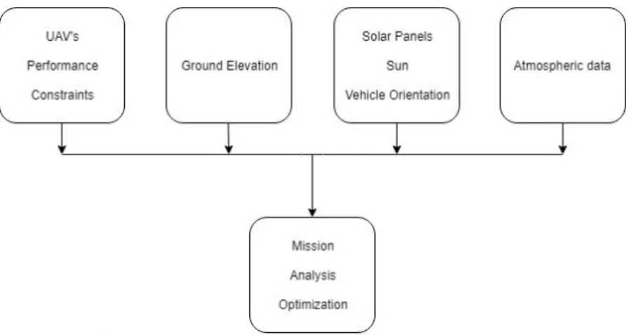
The main focus of the current chapter is to describe the chosen method to plan the mission for a solar powered UAV. For better understanding and organization during the development of this thesis, the method was divided in individual models. Each module will be described by Subsections along this chapter. In Figure 3.1 it can be seen the four models linked to one central box, these four models are independent subroutines that return the needed data to the main program. The main program is separated in two main phases, mission analysis and mission optimization. Starting with an analysis of a non-optimized initial mission (design variables), followed by an optimization phase, it calculates new design variables to optimize an objective function, taking in account some pre-defined constraints. The final optimized solution is found by an iterative process composed of a sequence of analyses and optimizations that is explained through this chapter.

Figure 3.1: Individual models used for the mission planning

3.1 Mission Analysis

The analysis phase purpose is to calculate the objective function and its constraints, from the design variables. The design variables are each latitude, longitude, altitude and airspeed of a set of waypoints that define the mission the user wants to plan. This is represented by Equation 3.1.

dv4n= (φ1, φ2, . . . , φn, λ1, λ2, . . . , λn, h1, h2, . . . , hn−1, hn, V1, V2, . . . , Vn)

φi, λi, hi, vi∈ Nfor1 ≤ i ≤ n (3.1)

(34)

lon-gitude, respectively) of each waypoint, h corresponds the altitude of flight at each waypoint measured from the take-off ground elevation and V is the airspeed at each waypoint. The num-ber of parameters is four times the numnum-ber of waypoints, n. There are two types of design variables: the first one is expressed in Eq. 3.1 in which the coordinates system is represented by the geographic coordinates represented in decimal degrees; the second one is represented by the Eq.3.2:

dv4n = (x1, x2, . . . , xn, y1, y2, . . . , yn, h1, h2, . . . , hn₋₁, hn, V1, V2, . . . , Vn)

xi, yi, hi, vi∈ Nfor1 ≤ i ≤ n (3.2)

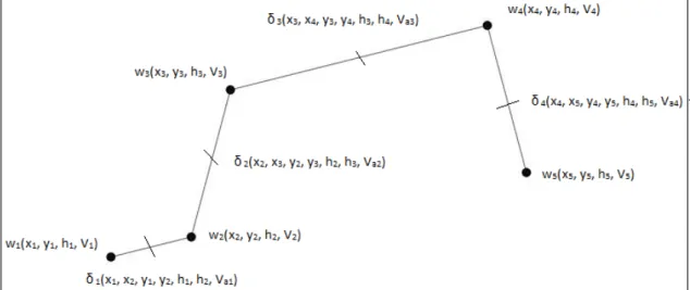
in which x and y are represented in the East North Up (ENU) coordinates. If the design variables are defined in the geographic coordinates format, the algorithm of analysis has to convert the coordinates to the ENU system, so the final inputs are in SI units. If the design variables are already defined in the second format the mission analysis will proceed. Figure 3.2 shows the Initial trajectory representation, where each waypoint represents each xi, yi and hi, where i

Figure 3.2: Initial 5 waypoints trajectory example.

is the waypoint index, the correspondent Vi is saved in the program in each waypoint vector.

The analysis is done by segment performance, which represents the segment performance δj of

flight between a waypoint wiand a waypoint wi+1. It is important to note that, in the following

equations, if the parameter is referent to a waypoint i is used as the parameter index. On the other hand, if the parameter is referent to a segment, it has j as the correspondent index. The next step of the analysis is to calculate each segment performance parameter, starting with the segment total distance, that is given by

dsj=

√

dg2j+ dh

2

j (3.3)

(35)

dg_j = √

(xj+1− xj)2+ (yj+1− yj)2 (3.4)

and, dhjis the segment height variation that can be written as

dhj = hj+1− hj (3.5)

The next step of the mission analysis algorithm is to calculate the average segment airspeed along the path, that is represented by,

Vaj=

Vj+1+ Vj

2 (3.6)

followed by the calculation of average segment wind speed components V waxj, V wayj,V wazj.

It should be mentioned that this step is dependent on the atmospheric data model. The model described in Section 3.6, will return to this step the wind speed V w at each waypoint and the corresponding angle of orientation θwi which assumes the north-clockwise convention, θwi

∈ [0, 360[ where 0 represents the North → South way.

So the average segment wind speed is given by:

V waj(V waxj, V wayj, V wazj) (3.7) where, V w_ax_j =V wxj + V wxj+1 2 (3.8a) V wayj = V wyj + V wyj+1 2 (3.8b) V w_az_j = V wzj + V wzj+1 2 (3.8c) and V wxi= V wicos(90− θwi) (3.9a) V wyi= V wisin(90− θwi) (3.9b) V wzi= 0 (3.9c)

The vertical wind speed component is considered zero due to weather forecast databases limita-tions, yet the model considered 3D components to be used if a more complete weather database is implemented in a next version of the software. Hence,

V waj = √ V waxj 2 + V wayj 2 + V wazj 2 (3.10)

(36)

Due to lack of the database information the angle of orientation of the wind speed, θwi, is two

dimensional (x, y), so V wazj is considered zero.

Once the average wind speed is calculated it is necessary to know the flight path direction. In Figure 3.3, between two waypoints ds, dgand dh are already known from Equations 3.3, 3.4

and 3.5 respectively, θgj and γgj are described bellow in equations 3.11 and 3.12.

Figure 3.3: Flight Path Direction Scheme

θgj = arctan ( yj+1− yj xj+1− xj ) = arcsin(dgyj dgxj ) (3.11) γgj = arctan dhj dsj (3.12)

With this, the next step is to calculate the average ground speed V gaj,

V gaj(V gaxj, V gayj, V gazj) (3.13)

where the average ground speed components along the path dsiare represented by,

V g_ax_j = V gajcos(γgj) cos(θgj) (3.14a)

V g_ay_j = V gajcos(γgj) sin(θgj) (3.14b)

V g_az_j = V gajsin(γgj) (3.14c)

(37)

⃗ V gaj = ⃗Vaj+ ⃗V waj ↔          V g_ax_j = Vaxj + V waxj V g_ay_j = Vayj+ V wayj V g_az_j = Vazj + V wazj (3.15)

where Vaxj,Vayj and Vazj are defined in Equations 3.16 - 3.18.

V_ax_j = V g_ax j− V waxj = V gajcos(γgj) cos(θgj)− V waxj (3.16) V_ay_j = V g_ay j − V wayj = V gajcos(γgj) sin(θgj)− V wayj (3.17) V_az_j = V g_az j− V wazj = V gajsin(γgj)− V wazj (3.18)

Adding the square of Equations 3.16, 3.17 and 3.18 it is obtained [V gajcos(γgj) cos(θgj)− V waxj] 2_{+ [V g} ajcos(γgj) sin(θgj)− V wayj] 2_{+ [V g} ajsin(γgj)− V wazj] 2_{= V}2 a j so V g_a2_j − 2[cos(γgj) ( cos(θgj)V waxj+ sin(θgj)V wayj ) + sin(γgj)V wazj]V gaj +[V w2_ax j + V w 2 ayj+ V w 2 azj − V 2 a j] = 0

and can be solved by

aV g2aj + bV gaj + c = 0

V gaj =

−b ±√b2− 4ac

2a (3.19)

where a, b and c are given by

a = 1 b = V w2_ax j+ V w 2 ayj + V w 2 azj− V 2 a j c = V w2_ax j+ V w 2 ayj + V w 2 azj− V 2 a j

At this phase the time in each segment can be calculated by,

dtj =

dsj

V gaj

(3.20)

and the total time can be expressed as:

ttotal= n_∑₋₁ j=1

(38)

Since the time of the mission is known, the analysis continues to calculate the missions energy. First, it has to be calculated the air path angle, γaj,

γaj = arcsin(

Va_zj

Vaj

) (3.22)

where Vazj also represents the rate of climb in each segment RCj.

For the calculation of aerodynamic forces, since in Equations 3.25 and 3.26 the speed variable is squared, the squared average velocity is represented in Equation 3.23.

V avej= √ V2 j + V 2 j+1 2 (3.23)

Therefore the aerodynamic forces and their coefficients (lift, Lj, drag, Dj, lift coefficient, CLj

and drag coefficient, CDj) are:

Lj= Wicos(γaj) cos(ϕbj) (3.24) CLj = Lj 1 2ρV ave 2 j (3.25) CDj = f (CLj) (3.26) Dj= 1 2ρV ave 2 jSCDj (3.27)

where Wjis the aircraft weight, ϕbj is the bank angle, S is the wing area and ρ is the air density.

More over the drag coefficient is calculated as a function of the lift coefficient multiplied by the values of the drag polar vector presented in Table 4.2. The next step of the analysis is to calculate the average acceleration, aj, the average inertial force, QIFj and the average rolling

friction force, Fj. Those can be calculated by

aj= V gaj+1 dtj (3.28) QIFj = Wj g aj (3.29) Fj= µj(Wj− Lj) (3.30)

where µj is the coefficient of ground rolling friction. Then the average required thrust is given

by

Tj = Dj+ Wjsin(γaj) + QIFj + Fj (3.31)

and finally the average required power Preqj, the average electric power, Pej and the consumed

(39)

Preqj = TjVaj (3.32)

Pelej = UjIj (3.33)

dEj = Pejdti (3.34)

where Ujand Ijare the input voltage and the motor current, respectively, and can be calculated

by an iteration process described in Section 3.4. Note that the energy here is the required energy for each segment. The energy system distribution between the photovoltaic panels (PV panels) and the battery is explained in Section 3.7.

3.2 Motor Performance Model

Electric motors, transform electrical power into mechanical torque and rotational speed. For this work, it is very important to understand how an electric motor works, since the motor is one of the major limitations of the aircraft.

The motor operating properties are defined by some independent parameters, usually specified by the manufacturer, namely: the electric current, I; the no load current, I0, that represents

the electric current when there is no load attached to the motor; the electric resistance, R; And the induced or effective voltage, Uef f [25].

Therefore, based on the model presented in [26], the induced voltage can be calculated as

Uef f = U− RI (3.35)

where U is the actual input voltage. Multiplying the induced voltage by the motor velocity constant, results in the motor speed,

Ω = Kv Uef f (3.36)

thus, the induced voltage can also be represented by

Uef f =

Ω

Kv. (3.37)

U is the overall voltage without considering losses due to resistance, and can be represented as a function of motor speed, Ω, and input current, I, according to

U (Ω, I) = Uef fΩ + I R =

Ω

Kv + I R (3.38)

Likewise that there are some voltage losses, the same happens with the total input current. Hence, the effective current, Ief f is given by

(40)

where the no load current, I0, does not contribute to useful torque. So the input current, I, can be represented as I = 1 R ( U− Ω Kv ) (3.40)

With the input current and voltage values known, it is possible to calculate the total electric power consumed, Pele, as

Pele= U I (3.41)

Following the same logic and considering Ief f and Uef f, the effective power remaining after

the power losses, Pef f, is given by

Pef f = Uef fIef f (3.42)

The available torque at the shaft, Qm, can be represented by Equation 3.43 based on the power

and torque relation.

Qm=

Pef f

Ω (3.43)

Lastly, the motor efficiency, ηmotor, is obtained by the ratio of the effective power and the

overall power converted.

ηmotor =

Pef f

Pele

= Ief fUef f

I U (3.44)

3.3 Propeller Performance Model

For the correct simulation of the propulsion system, it is necessary to consider a propeller per-formance model, as complement to the electric motor perper-formance model. For this purpose, the propeller performance model presented in reference [26] was implemented.

To complement the electric motor performance model, it is necessary to calculate the pro-peller efficiency, ηprop, and the power coefficient, Cp. These depend on the propeller advance

ratio, Jprop, which is a non-dimensional parameter and is defined by

Jprop=

60.V

N d (3.45)

where V is the linear velocity of the propeller, with respect to the flow field, N is the propeller speed in revolutions per minute, and d is the propeller diameter. Notice that N/60 represents the propeller speed in revolutions per second rps.

By knowing how the power coefficient Cp varies with the advance ratio Jprop, it is possible

to calculate the propeller shaft power Pshaf t, as:

Pshaf t= Cpρ ( N 60 )3 d5 (3.46)

(41)

For the calculation of the power coefficient, Cp, and the propulsive efficiency, ηp, as functions of

the propeller advance ratio, Jprop, for a single propeller with a fixed diameter, d, and pitch, p, a

polynomial approximation was used presented in reference [26]. This polynomial approximation is defined by Cp = Cp0× [ A0+ 4 ∑ i=1 ( Ai ( Jprop Jmax )i)] (3.47) ηp= ηpmax× [ B0+ 6 ∑ i=1 ( Bi ( Jprop Jmax )i)] (3.48)

where Cp0 is the power coefficient at a null advance ratio, ηpmax is the maximum propeller

efficiency, Jmax is the maximum advance ratio, A and B are the coefficient vectors obtained

through the polynomial approximation. The coefficients used in this work are:

A =              0.9999747473830 0.0026886303943 −0.0542821394531 −0.8141198610786 0.2382888347204 −0.1060271581734 0.0222789611099              (3.49) B =              0.0000000000000 2.8358158896651 −4.6740787983266 17.2094772778345 −45.734194221401 55.789219497612 −25.395785093511              (3.50)

Jmax, ηpmax and Cp0 are obtained by

Jmax= C1d + C2p + C3d2+ C4dp + C5p2+ C6d3+ C7d2p + C8dp2+ C9p3 (3.51) Cp0 = D1d + D2p + D3D 2_{+ D} 4dp + D5p2+ D6d3+ D7d2p + D8dp2+ D9p3 (3.52) ηpmax= E1d + E2p + E3d 2_{+ E} 4dp + E5p2+ E6d3+ E7d2p + E8dp2+ E9p3 (3.53)

(42)

where the coefficient vectors C, D and E are C =                      0.706462000000 −0.046405100000 0.074350100000 0.001069860000 −0.001664110000 −0.000007715000 −0.000006521000 0.000008688670 0.000002563530 −0.000000703183                      (3.54) D =                      0.050916200000 −0.005511640000 0.007489280000 0.000144156000 −0.000239091000 0.000065509200 −0.000002407300 0.000005544700 −0.000003824100 0.000000875200                      (3.55) E =                      0.375474000000 0.013321100000 0.014884800000 −0.000358479000 0.000020627100 −0.000189967000 0.000003644830 −0.000004047110 0.000004028760 −0.000000467311                      (3.56)

Note that the coefficients were obtained from the model presented in [26], and refers to the propeller of the UAV used to verify the mission planner software.

3.4 Mission’s Power and Energy Model

Based on Sections 3.2 and 3.3, this Section describes the model used to calculate the parame-ters needed for the analysis and optimization of the mission. Those parameparame-ters are the motor power setting, δset, the motor speed, Ω, and the input voltage, U .

(43)

equal the motor shaft power. Given an assumed δ, this subroutine allows the calculation of the input voltage, the motor speed and the motor shaft power, Pshaf t, by adjusting the motor

current, I, through an iterative process, in order to match the condition of the propeller-motor matching. For a minimum electric power required, the propeller must assume a value that equals the required power calculated by Equation 3.32. By these means, the motor setting is corrected and adjusted through an iterative process, to match the condition of a minimum electric power required, where the propeller must assume a value as minimum as possible, con-sequently equalling the required power for levelled flight.

This subroutine is called after the calculation of the segment required power, Preqj, Equation

3.32. When this subroutine finishes, the mission analysis process can proceed to the calculation of Pelej and Ej. Equations 3.33 and 3.34, based on this subroutine it can be written as

Pelej = ( U I + (RESCI2+ RUI2) ) jnmotor (3.57) (3.58)

where RU, is the battery resistance and RESC, is the motor speed controller resistance. These

must be considered due to the energy losses in the consumed electric power.

Note that the energy used by the aircraft’s electrical systems must be added to Equation 3.57 to calculate the total electric power in each segment.

PTj = Pelej + Psysj (3.59) dEj = PTjdt (3.60) E = n ∑ 1 (dEj) (3.61)

Where n is the number of segments.

3.5 Ground Elevation Model

One of the most important features of a mission planner is to be able to detect an obstacle and be able to make the necessary corrections to avoid the obstacle. Thus, the ground elevation model is responsible for providing the necessary ground elevation data to the analysis routine. With this purpose, a free and open-source Application Programming Interface (API) database was choosen to map the ground elevation. All public API instructions documentation is available in [27].

The latitude and longitude of a point on earth (input data) is sent to the API as a request and consequently, it will return the elevation at this point (output). The algorithm that achieves this is described bellow. It starts by defining the boundaries, the user needs to define two points that represent the initial and ending point of the diagonal of the desired map.

Q11(Qlat1, Qlon1) (3.62)

(44)

where Q11 and Qm are the initial and the ending point of one of the map’s diagonals. Notice

that,

{φ1, φ2, . . . , φn} ⊂] Qlat1, Qlatm[ (3.64)

{λ1, λ2, . . . , λn} ⊂] Qlon1, Qlonm[ (3.65)

where φ1, φ2, . . . , φmand λ1, λ2, . . . , λm are the latitudes and longitudes of the mission’s

way-points, respectively, n is the number of waypoints and assuming the map as a matrix m× m, so m is the number of points requested by column of the map, and so representing the resolu-tion of the map. Once n is defined it is created a 2D matrix, where Qlat1 and Qlatndefine the

N orth→ south boundaries as well as Qlon1 and Qlonn are the W est→ East boundaries of the

map. Then n2 _{number of points will be sent to the database as a request for each elevation,}

resulting in a grid with n2 _{three-dimensional points Q}

Elevation(Qlati, Qloni, Qelei). The data is

saved as a list of the points in three columns, each line representing a three dimensional point

QElevation. Finally, the file is saved as earth elevation in a .txt format. Now that the elevation

data is known and saved, the main program has access to this through a subroutine, where the data is read from the earth elevation file and saved in a three dimensional vector. With all the necessary data from elevation API saved in the program, the process that achieves the elevation of a pair of coordinates is simple, firstly the vector is searched to find the four nearest points to the input coordinates P = (x, y). This is represented graphically in Figure 3.4.

Figure 3.4: The four red dots show the data points and the green dot is the point at which we want to interpolate.

Notice in Figure 3.4 and in the following description of the interpolation’s algorithm x and y represent the latitude and longitude of the ground points, respectively. Secondly having four points, Q11 = (x1, y1), Q12 = (x2, y1), Q21 = (x1, y1) and Q22 = (x1, y1), and knowing the

elevation value correspond to each of the four points Qii, f (P (x, y)) can be interpolated by

(45)

f (x, y1)≈ x2− x x2− x1 f (Q11) + x− x1 x2− x1 f (Q21) (3.66) f (x, y1)≈ x2− x x2− x1 f (Q12) + x− x1 x2− x1 f (Q22) (3.67)

and then proceeding with the interpolation in the y-direction to obtain the desired estimate:

f (x, y)≈ y2− y y2− y1 f (x, y1) + y− y1 y2− y1 f (x, y2) = y2− y y2− y1 ( x2− x x2− x1 f (Q11) + x− x1 x2− x1 f (Q21) ) + y− y1 y2− y1 ( x2− x x2− x1 f (Q12) + x− x1 x2− x1 f (Q22 ) = 1 (x2− x1)(y2− y1) (f (Q11)(x2− x) + f(Q21)(x− x1)(y2− y) + f(Q12)(x2− x)(y − y1) + f (Q22)(x− x1)(y− y1)) = 1 (x2− x1)(y2− y1) [ x2− x x − x1 ] [_{f (Q} 11) f (Q12) f (Q21) f (Q22) ] [ y2− y y− y1 ] . (3.68)

Note that if the interpolation had started through the y-direction and then through the x-direction we would have reached the same result. Once the interpolation is done the subroutine returns the interpolated elevation to the main program.

3.6 Atmospheric Data Model

To make the mission planner viable the atmospheric data model is used to provide the mission’s atmospheric data (wind speed, wind direction, temperature deviation and the cloud cover). To achieve that, we choose the OpenWeatherMap API [28], which returns a five days forecast by geographic coordinates. This model is very similar to the ground elevation model, the method to request the data from the database is the same with a particularity: the database instead of returning three-dimensional points QElevation(Qlati, Qloni, Qelei), it returns six-dimensional

points QW eather(Qlati, Qloni, Qwindspeedi, Qwinddirectioni, QT empi, Qcloudsi). At this point, the data

is read through a subroutine responsible for the weather data and each variable of atmospheric data is interpolated for the mission’s analysis by the same method of 2D interpolation described on the ground elevation model Section. It is important to note that the database does not have data of vertical wind or the variation of the weather parameters through the altitude. So, this work considers the weather parameters constant in altitude, except for temperature, that is estimated calculating the temperature deviation referent to the International Standard Atmosphere (ISA) model.

(46)

3.7 Solar Model

The solar energy that the PV panel can harvest depends on its area, SP V, on the solar

irradia-tion J (or solar power per unit area) reaching it, and on its efficiency, ηP V. The atmosphere

is a strong influence on it, as well as the percentage of clouds. The Irradiation varies with the location on earth (mostly with latitude), with the orientation of solar panels and with the so-lar zenith angle (defined by the angle between the direction of the Sun’s centre and the local zenith). The zenith angle vary with the day of the year and hour of the day.

3.7.1 Estimated Solar Irradiance

Based on Ref. [29], the Solar Power per unit area can be estimated by

J = J0nτ sin(ζ), (3.69)

where τ is the transmittance factor, which is the ratio of the total radiant or luminous flux transmitted by a transparent object to the incident flux, ζ is the zenith angle and J0n is the

intensity of the extraterrestrial normal solar radiation which is given by

J0n= JSC ( rES,0 rES )2 , (3.70)

where JSC is the extraterrestrial normal solar radiation constant, rES,0 and rES are the mean

and real distances between the Earth and the Sun respectively. rES is a function of rES,0, the

eccentricity of Earth’s orbit, ε, and the true anomaly, v, which represents an angular param-eter that defines the position of a body moving along a Keplerian orbit. So, the real distances between the Earth and the Sun is expressed as

rES= rES,0 ( 1− ε2 1 + ε cos(v) ) , (3.71)

and the true anomaly, v, can be calculated by

v = 2πdn− 4

365 (3.72)

where dnis the day of the year, counting from the first of January (day 1). With J0n Known it is

necessary to calculate the zenith angle, which is given by

ζ = π

2 − arccos(sin(φ) sin(δs) + cos(φ) cos(δs) cos(µH)), (3.73)

where φ is the latitude of the location and δsand µH are the solar declination angle and the

hour angle respectively, which are calculated by

δs= 23.45π 180 sin ( 360284 + dn 365 ) , (3.74)

(47)

and

µ(H) = π− πH

12 (3.75)

where H is the hour of the day. The constants used in this model are listed in Table 3.1.

Table 3.1: The constant values used in Eqs. above. Symbol Value/unit

τ 0.85

JSC 1367 W/m2

rES,0 149,597,896 km

ε 0.0167

It is important to note that before sunrise and after sunset some output values for solar irradi-ance may be negative, so in this case they will be set to zero.

3.7.2 Cloud Cover Effect

As written in the previous Subsection, the energy that a PV panel can harvest is influenced by the clouds. Clouds are one of the largest attenuating factors of solar irradiance. Cloud cover is a useful predictor of solar resource. If the sky is cloudless, irradiance can be predicted from the solar geometry, surface albedo, and optical properties of aerosols, ozone and water vapour using a radiative transfer calculation. Alternatively, several clear-sky models exist in the liter-ature which are empirical relationships between one or more atmospheric variables [30]. The statistics of clear-sky index can be used to determine solar irradiance when the theoretical clear sky irradiance and the cloud cover are known. Based on clear-sky index model on Ref. [30], there is an empirical relationship between the clear-sky index Kcand cloud cover, Ccin (oktas),

thus the clear-sky index - cloud cover relationship is,

KC(Cc) = 1− 0.75(Cc/8)3.4 (3.76)

The solar irradiance harvested, considering the cloud effect, is given by

Jcloud= J KC (3.77)

3.7.3 Solar Power with Tilt Angles

With the solar irradiance and the cloud cover effect known, aircraft attitude must be considered, because the energy that the PV panels can harvest varies with angle of incidence of the sun, on the panels. Based on models from reference [31], we can find the relation between sun incidence and the PV panels. Knowing the solar declination angle δs, the hour angle H and the

(48)

Az, that is given by Equation 3.78 from reference [32].

Az =sin(ω) cos(δs)

sin(θZ)

(3.78)

The scheme used to calculate the sun’s Azimuth is illustrated in Figure 3.5.

Figure 3.5: Illustration of the sun’s position.

Then with the solar azimuth angle known, the angle of incidence θiof the Sun on a surface tilted

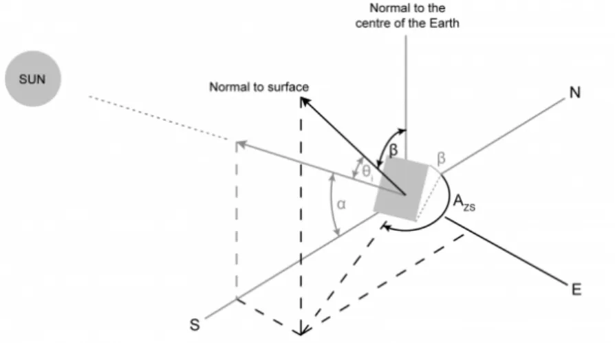
at an angle from the normal to the centre of the Earth, β and with any surface azimuth angle

AZS (Figure 3.6 ) can be calculated from (when AZS is measured clockwise from north):

cos(θi) = cos(90− ζ)cos(Az − Azs) sin(β) − cos(ζ) cos(β)

Figure 3.6: Illustration of the problem.

Then the solar irradiance on a tilted surface is given by

JT S= J cos(θi) (3.79)

(49)

itself. Finally, the total energy that the PV panels can harvest is given by

Esolar|total=

∫ tf

t

J KCSP V ηP V cos(θi) dt. (3.80)

3.7.4 Management of Electric Power Flow

The UAV used in this thesis has a parallel systems installation. The systems power distribution is described in Figure 3.7.

Figure 3.7: Systems Power distribution.

In this type of installation, the battery power is only used to compensate the lack of energy harvested by the PV panels. In the case of the total required power (motor required power plus the systems required power) being greater than the solar power, the used battery power is equal to

Pbat= Pmotor+ Psystem− Psolar (3.81)

on the other hand

Psolar= Pmotor+ Psystem− Pbat (3.82)

This energy management is assured by a subroutine called SystemsElectricManagement(). The subroutines algorithm is described in the following pseudocode.

(50)

Figure 3.8: Pseudocode for the management of the electrical Systems.

Notice that, when the solar power is greater than the required power, the battery consumption gets a negative value, this means that the battery is being charged.

3.8 Mission Optimization

The calculation of a optimal mission for aerial vehicles is the main objective of this dissertation. The mission planner was created based on FORTRAN Feasible Sequential Quadratic Programming (FFSQP) optimization algorithm. With the aircraft data and the design parameters stated in Equation 3.1 known, the program will be able to calculate the objective function and then proceed with its optimization. The three available options are the mission time, the mission energy and the mission distance. So, minimizing one of the three, is the objective function, which directly depends of the design variables and the mission constraints set at the beginning. Once the design parameters and the mission constraints are defined, the program proceeds with the analysis of a pre-defined mission, described in Section 3.1 to calculate the value of the objective function. After that, it is all set to the application of the optimization software. Figure 3.9 describes this process.

Figure 3.9: Iterative process flowchart.

3.8.1 FFSQP Subroutines

For the optimization stage, a set of FORTRAN subroutines are used for the minimization of the objective functions, subject to general smooth constraints (if there is no objective function, the goal is to simply find a point satisfying the constraints) [33]. These set of constraints may be nonlinear or linear equality and inequality constraints, where the design variables are limited by these boundaries. FFSQP applies the Sequential Quadratic Programming methodology for

Mission Planner for Solar Powered Unmanned Aerial Vehicles

UNIVERSIDADE DA BEIRA INTERIOR

Engenharia