Persistence change in tourism data
JORGE M.L.G. ANDRAZ
Faculty of Economics, Universidade do Algarve and CASEE, Campus de Gambelas, 8005-139 Faro, Portugal. E-mail: [email protected].
PAULO M.M. RODRIGUES
Banco de Portugal, Universidade Nova de Lisboa and CASEE, Av. Almirante Reis, 71, 6º, 1150-012 Lisbon, Portugal. E-mail: [email protected].
The authors apply recently proposed persistence change tests to inbound tourism series in order to evaluate whether their properties have changed over time. By using quarterly series of the number of overnight stays in hotel accommodation and similar establishments in the Algarve, from 1987:01 to 2008:03, they gathered evidence of persistence change in all series. In particular, a change from I(1) to I(0) was detected for some countries, while for others the direction change was not clear-cut. These results have implications from a policy perspective and shed light on the generally accepted conviction that policy decision processes should not ignore the fact that, in general, tourism inbound series display mean reverting behaviour, being only temporarily affected by external shocks. Keywords: persistence change; non-stationarity; stationarity; tourism demand
JEL classification: C12; C22
Testing for the presence of a unit root is now routine practice in empirical research given the different statistical and economic implications of classifying a series as stationary or non-stationary. Establishing this distinction is mean-ingful in that it helps in understanding the effects of shocks on macroeconomic variables. While the impact of shocks will be transitory for a stationary series, for a non-stationary one any random shock may have persistent effects. In other words, while a stationary time series will display mean reverting behaviour, a non-stationary variable will display persistent behaviour; that is, shocks will have long-lasting effects, thus preventing the series from returning to any defined level.
We thank Professor Carlos Barros and two anonymous referees for their useful comments and suggestions. Financial support from POCTI/FEDER (grant reference PTDC/ECO/64595/2006) is also gratefully acknowledged.
Therefore, the study of the statistical properties of time series has attracted a great deal of attention because of their implications on model building and forecasting in applied macroeconomics and finance. A great effort has been concentrated mainly on variables such as inflation whose statistical properties have been analysed in a large number of empirical and theoretical papers published recently in the literature (see among others Fuhrer and Moore, 1995; Gibson and Lazaretou, 2001; Johnson, 2002; Galí et al, 2003; Steinsson, 2003; Angeloni et al, 2006; Batini, 2006; Dotsey and King, 2006). Two broad reasons have motivated this upsurge. First, inflation has been a key variable of the monetary policies followed in European countries that have adopted inflation-targeting regimes in the context of their adhesion to the European Monetary Union. Second, the evolution of GDP has been widely analysed with multiple purposes, as it plays a key role in the catching-up process involving European countries. However, in recent years, it has been observed that macroeconomic variables may display both stationary and non-stationary features within a specific period; see, for instance, Halunga et al (2009). Indeed, it seems that some series could be switching from I(0) to I(1) behaviour, or vice versa.
Parallel to macroeconomic variables and with direct implications on a country’s macroeconomic performance, tourism activity has revealed itself as one of the world’s largest and fastest growing industries, playing a key role in the economic growth of many countries, lending itself to other economic sectors through direct and indirect multiplier effects. Portugal relies heavily on this industry as an important means of (economic) resource, catering largely to the European market. In 2006, the country was visited by 12.8 million tourists, being responsible for 5% of GDP and 10% of employment. The increasing number of tourists and their strategic importance, in terms of revenue and employment, as well as in terms of direct and indirect effects on several other economic sectors, has led economic agents to adopt important dynamic measures in relation to supply. Portugal has been able to keep its international market share despite the growing number of competing markets that are once again attracting tourists to traditional destinations.
The strategic importance of tourism has contributed decisively to extensive research on its effects on the economic performance of Portugal, whose reliability imposes a careful analysis of the statistical properties of the series. On the other hand, assessing its persistence by quantifying the response of tourism to shocks hitting the economy is crucial for the implementation of efficient policies towards the sector. In particular, quantifying the sluggish response of tourism to changes in economic conditions or others appears as a fundamental prerequisite if the government aims to implement a policy strategy towards the sector’s development. Furthermore, and in order to understand the determinants of tourism demand behaviour better, it would be relevant to be able to identify whether tourism inflows follow a stationary process, allowing for the possibility of variations in the degree of persistence due to changes in the structure of the economy or in policies towards the sector.
This paper contributes to the literature by analysing whether the persistence of tourism has changed over the period 1987–2008, by employing the tests of Kim (2000) and Harvey et al (2006). The results suggest that tourism inflows to Portugal may have undergone a structural change, having switched from non-stationary to non-stationary behaviour.
The paper is organized as follows. The next section reviews the statistical procedures to test for changes in persistence of tourism inflows to Portugal. The subsequent two sections, respectively, present finite sample results of the performance of the persistence change tests when applied to seasonally unadjusted data, and provide the empirical results. Finally, we offer our conclusions.
Methodological framework
The persistence change model
For the purpose of presenting the persistence change tests, we follow Harvey et al (2006) and Busetti and Taylor (2004) and consider the following data-generation process,
yt = xt′ β + vt (1)
vt = ρtvt–1 + εt , t = 1,...,T (2)
with v0 = 0. In (1), xt is a set of deterministic variables, such as seasonal dummies only or seasonal dummies and a time trend. The vector xt is assumed to satisfy the mild regularity conditions of Phillips and Xiao (1998), and the innovation sequence {εt} is assumed to be a mean zero process satisfying the familiar α-mixing conditions of Phillips and Perron (1988, p 336) with strictly positive and bounded long-run variance, ω2 ≡ lim
T→∞ E( T Σ t=1εt)
2 (see Harvey et al,
2006, p 444). In (1)–(2), considering the zero frequency roots only, four hypotheses can be considered:
(1) H1: yt is I(1) (that is, non-stationary) throughout the sample period; (2) H01: yt is I(0) changing to I(1) (in other words, stationary changing to
non-stationary) at time [τ*T]. The change point proportion is assumed to be
an unknown point in Λ = [τl,τu], an interval in (0,1) which is symmetric around 0.5;
(3) H10: yt is I(1) changing to I(0) (that is, non-stationary changing to station-ary) at time [τ*T];
(4) H0: yt is I(0) (stationary) throughout the sample period.
Ratio-based tests
In order to test the hypotheses in (1)–(4), Kim (2000), Kim et al (2002) and Busetti and Taylor (2004) have developed tests for the constant I(0) data-generating process (DGP) (H0) against the I(0)–I(1) change DGP (H01), which are based on the ratio statistic,
(T – [τT])–2 ΣT t=[τT]+1(Σ t i=[τT]+1 ~ υi,τ)2 K[τT] = –––––––––––––––––––––––––––– (3) [τT]–2 Σ[τT] t=1(Σ t i=1 ^ υi,τ)2 where υ^
t,τ is the residual from the OLS regression of yt on xt for observations up to [τT] and υ~
t = [τT],…,T. For example, in the seasonal dummy case, xt is an S × 1 vector, with 1 corresponding to season s, s = 1,…S and zero everywhere else, υ^t,τ = yt – y–
s(τ), with y–s(τ) corresponding to the mean of season s over the subsample t = 1,…,[τT].
Since the true change point, τ*, is assumed unknown, Kim (2000), Kim et al (2002) and Busetti and Taylor (2004) consider three statistics based on the sequence of statistics {K(τ),τ ∈ Λ}, where Λ = [τl, τu] is a compact subset of [0,1], that is, [τuT] K1 = T*–1 Σ K(s/T) (4) s=[τlT] [τuT] 1 K2 = lnT*–1 Σ exp – K(s/T) (5) s=[τlT] 2 K3 = max K(s/T) (6) s∈{[τlT],...,[τuT]}
where T* = [τuT] – [τlT] + 1 and τl and τu correspond to the (arbitrary) lower and upper values of τ* (in the empirical section, we set τl = 0.2 and τu = 0.8, as is frequently adopted in the literature). Limit results and critical values for the statistics in (4)–(6) can be found in Harvey et al (2006).
Note that the procedure in (4) corresponds to the mean score approach of Hansen (1991); (5) is the mean exponential approach of Andrews and Ploberger (1994); and, finally, (6) is the maximum Chow approach of Davies (1977) (see also Andrews, 1993).
In order to test H0 against the I(1)–I(0) change DGP (H10), Busetti and Taylor (2004) propose further tests based on the sequence of reciprocals of Kt, t = [τlT],…,[τuT]. They define KR
1, K
R
2 and K
R
3 as the respective analogues of
K1, K2 and K3, with Kj, j = 1,2,3 replaced by K–1j throughout. Furthermore, to
test against an unknown direction of change (that is either a change from I(0) to I(1), or vice versa), they also propose KM
i = max[Ki, K R
i], i = 1,2,3. Thus, tests which reject for large values of K1, K2 and K3 can be used to detect H01, tests which reject for large values of KR
1, K
R
2 and K
R
3 can be used to detect H10, and
tests which reject for large values of KM
1, K
M
2 and K
M
3 can be used to detect
either H01 or H10.
Modified ratio-based test
As noted by Harvey et al (2006), all statistics previously presented possess pivotal limit distributions under both H0 and H1. Thus, they employ the approach of Vogelsang (1998) to produce tests based on modified versions of these statistics which, for a given test and significance level, have the same critical value in the limit as the corresponding unmodified test under H0, but where the same limit critical value is also appropriate under H1.
The modification is largely the same for all tests. In other words, following Vogelsang (1998) and Harvey et al (2006), a modified variant of Ki can be considered as,
Kim = exp(–biJ1T)Ki, i = 1,2,3
where bi, i = 1,2,3 are finite constants and J1T is a T–1 times the Wald statistic
for testing the joint hypothesis γk+1 = … = γ9 = 0 in the regression,
yt = xt′ β + Σ9 i=k+1 γit
i + error, t = 1,...,T.
Note that J1T is the unit root test statistic proposed by Park and Choi (1988) and Park (1990), which is used to test explicitly for zero frequency non-stationarity of {yt}. This statistic will serve as an activation mechanism of the correction factor exp(–bi J1T). This results from the fact that if the series is stationary, asymptotically, J1T → 0 and hence exp(–bi J1T) → 1, whereas if the series is non-stationary, J1T will not converge to zero, therefore inducing exp(–biJ1T) to provide the necessary scaling to adjust the critical value.
Harvey et al (2006) also suggest a variant of this modification procedure, which is perhaps more natural to consider when testing against H01 by replacing the correction factor J1T with Jmin = minτ∈Λ J1,[τ T] where J1,[τ T] is T–1 times the
Wald statistic for testing the joint hypothesis γk+1 = … = γ9 = 0 in the regression
yt = xt′ β + Σ9 i=k+1 γit
i + error, t = 1,...,[τ T]. Note that for the reciprocal statistics, the JR
min correction is given from J
R
min =
minτ∈Λ J[τ T]T, where J[τ T] is T–1 times the Wald statistic for testing the joint
hypothesis γk+1 = … = γ9 = 0 in the regression yt = xt′ β + Σ9
i=k+1 γit
i + error, t = [τ T],...,T.
Furthermore, as regards the test against an unknown direction of change, the two modifications suggested by Harvey et al (2006) to KM
i are defined as, KM i, J = exp(–bMi J1,T)KMi and KM i, min = exp(–b Mτ i min[ Jmin, J R min])K M i , i = 1,2,3.
Regarding the necessary b values to implement the tests presented in this section, we refer to Harvey et al (2006, p 453), who provide a table with the asymptotic b values for modified tests of stationarity or a unit root against a change in persistence.
Finite sample performance of the persistence change tests Harvey et al (2006) present an in-depth study of the empirical size and power performance of the persistence change tests previously introduced in the context of non-seasonal data. In this section, we complement that analysis by looking at the behaviour of the tests when applied to seasonal data.
For the purpose of our Monte Carlo study, we consider the following DGP,
yt = xt′ β + vt (7)
(1 – ρ0tL)(1 – ρ1tL)(1 – ρ2tL2)ν
t = εt, t = 1,...,T (8)
with ν–3 = … = ν0 = 0. In (7), xt is a deterministic kernel (such as seasonal dummies only or seasonal dummies and a time trend), εt ~ nid(0,1) and ρit = {0,1}, i = 0,1,2. The critical values used in our analysis were taken from Harvey et al (2006, Table 1, p 451).
Tables 1 and 2 present the empirical size and power of the Ki, KR i and K
M i, i = 1,2,3 tests. The lines with numbers in bold represent the power of the zero frequency (long-run) persistence change tests and the remaining correspond to the empirical size. From the analysis of these two tables, we observe that although at times empirical size exceeds the nominal size considered, it is generally acceptable. The more severe size distortions are observed when a change from I(1) to I(0) at the Nyquist frequency and from I(0) to I(1) at the annual frequency is considered simultaneously. This is particularly severe when seasonal demeaning and detrending is considered (note that an empirical size of 36% is observed). It should be noticed, however, that the results refer to the cases where ρit = {0,1}, i = 1,2,3 and that if ρit< 1, the empirical size of all tests would be smaller or equal to 5%,1 which is an encouraging result
given that existing empirical evidence in the literature is not supportive of the full set of seasonal unit roots (see Osborn, 1990), neither are the results presented in Table 3 (see next section) for the series under analysis.
Note, however, that further analysis needs to be carried out in order to understand the properties of these tests better when applied to the seasonal context.
Empirical results
Properties of tourism data
For the purposes of empirical analysis, we consider the number of overnight stays in hotel accommodation and similar establishments in the Algarve by tourists from the UK, Germany, the Netherlands, Ireland, Portugal and Spain. The sample period considered is from the first quarter of 1987 to the third quarter of 2008 (87 observations). The data are taken from statistics published by the Portuguese Office for National Statistics.
Figure 1 presents the graphs of the natural logarithms of the series for the six countries under analysis. To get a clearer picture of the series, we present their seasonally demeaned and seasonally demeaned and detrended representations in Figure 2. A visual inspection suggests that all series exhibit non-stationary behaviour for the full sample. After an increasing trend, the series of tourism from the UK seems to be stationary from 2000 onwards. For Germany, an increasing trend over the first half of the sample is followed by a decreasing trend in the second half. The non-stationarity also seems to be present in the series of the Netherlands, Ireland and Portugal, showing increasing trends, while for Spain the trend is much less pronounced.
T
able 1.
Empirical size and power of persistence change tests – seasonally demeaned case.
ρρρρρ0 ρρρρρ1 ρρρρρ2 K1 K2 K3 K R 1 K R 2 K R 3 K M 1 K M 2 K M 3 [1; τττττ T ][ τττττ T ;T ] [1; τττττ T ][ τττττ T ;T ] [1; τττττ T ][ τττττ T ;T ] 0 0 0 0 0 0 0.056 0.056 0.056 0.055 0.053 0.053 0.062 0.053 0.053 10 0 0 0 0 0.208 0.383 0.385 0.977 0.978 0.976 0.969 0.971 0.970 01 0 0 0 0 0.985 0.983 0.981 0.144 0.285 0.289 0.979 0.976 0.975 0 0 0 1 0 0 0.042 0.044 0.048 0.056 0.054 0.055 0.046 0.048 0.051 0 0 1 0 0 0 0.071 0.067 0.066 0.012 0.035 0.040 0.039 0.053 0.056 0 0 0 0 1 0 0.053 0.033 0.055 0.037 0.073 0.080 0.042 0.070 0.073 0 0 0 0 0 1 0.037 0.039 0.043 0.042 0.042 0.042 0.036 0.036 0.039 0 0 1 0 1 0 0.134 0.122 0.125 0.010 0.033 0.038 0.077 0.081 0.085 0 0 0 1 0 1 0.007 0.015 0.018 0.106 0.088 0.090 0.059 0.055 0.057 0 0 0 1 1 0 0.043 0.058 0.061 0.040 0.105 0.114 0.035 0.093 0.099 0 0 1 0 0 1 0.075 0.187 0.201 0.087 0.191 0.205 0.082 0.229 0.237 0 0 1 1 0 0 0.049 0.047 0.048 0.053 0.044 0.048 0.047 0.046 0.047 0 0 0 0 1 1 0.029 0.026 0.029 0.027 0.027 0.032 0.025 0.025 0.027 Note :
Results are computed from the application of the persistence change tests to seasonally demeaned data. A 5% nominal size was c
onsidered,
T
= 100 and
τ
T
able 2.
Empirical size and power of persistence change tests – seasonally demeaned and detrended case.
ρρρρρ0 ρρρρρ1 ρρρρρ2 K1 K2 K3 K R 1 K R 2 K R 3 K M 1 K M 2 K M 3 [1; τττττ T ][ τττττ T ;T ] [1; τττττ T ][ τττττ T ;T ] [1; τττττ T ][ τττττ T ;T ] 0 0 0 0 0 0 0.057 0.060 0.059 0.051 0.052 0.054 0.052 0.054 0.056 10 0 0 0 0 0.390 0.569 0.589 0.992 0.992 0.989 0.985 0.986 0.983 01 0 0 0 0 0.980 0.983 0.979 0.199 0.427 0.467 0.973 0.980 0.976 0 0 0 1 0 0 0.119 0.110 0.105 0.046 0.048 0.051 0.099 0.087 0.085 0 0 1 0 0 0 0.058 0.060 0.061 0.068 0.102 0.124 0.070 0.101 0.119 0 0 0 0 1 0 0.040 0.038 0.041 0.044 0.073 0.095 0.040 0.065 0.081 0 0 0 0 0 1 0.094 0.084 0.087 0.025 0.028 0.036 0.070 0.062 0.070 0 0 1 0 1 0 0.109 0.098 0.094 0.012 0.031 0.049 0.064 0.067 0.078 0 0 0 1 0 1 0.024 0.021 0.028 0.084 0.070 0.075 0.055 0.044 0.051 0 0 0 1 1 0 0.102 0.104 0.108 0.073 0.117 0.143 0.103 0.135 0.154 0 0 1 0 0 1 0.188 0.297 0.359 0.182 0.261 0.305 0.227 0.339 0.380 0 0 1 1 0 0 0.113 0.101 0.091 0.107 0.096 0.090 0.145 0.123 0.113 0 0 0 0 1 1 0.060 0.051 0.052 0.064 0.053 0.055 0.067 0.055 0.059 Note :
Results are computed from the application of the persistence change tests to seasonally demeaned data. A 5% nominal size was c
onsidered,
T
= 100 and
τ
Figure 1.
Logs of overnight stays by country of origin.
UK
Germany Ireland Spain
The Netherlands Portugal 1988 1990 1992 1994 1996 1998 2000 2002 2004 2006 2008 1988 1990 1992 1994 1996 1998 2000 2002 2004 2006 2008 1988 1990 1992 1994 1996 1998 2000 2002 2004 2006 2008 1988 1990 1992 1994 1996 1998 2000 2002 2004 2006 2008 1988 1990 1992 1994 1996 1998 2000 2002 2004 2006 2008 1988 1990 1992 1994 1996 1998 2000 2002 2004 2006 2008 14.6 14.4 14.2 14.0 13.8 13.6 13.4 13.2 13.0 14.2 13.8 13.4 13.0 12.6 12.2 11 .8 11 .4 11 .0 13.4 13.0 12.6 12.2 11 .8 11 .4 11 .0 14 13 12 11 10 9 8 14.6 14.2 13.8 13.4 13.0 12.6 12.2 11 .8 11 .4 12.6 11 .8 11 .0 10.2 9.8 9.4 9.0
Figure 2.
Demeaned and detrended logs of overnight stays by country of origin.
Note
:
The solid line corresponds to the seasonally demeaned data and the dashed line to the seasonally demeaned and detrended data.
UK Germany The Netherlands Ireland Spain Portugal 1988 1990 1992 1994 1996 1998 2000 2002 2004 2006 2008 1988 1990 1992 1994 1996 1998 2000 2002 2004 2006 2008 1988 1990 1992 1994 1996 1998 2000 2002 2004 2006 2008 1988 1990 1992 1994 1996 1998 2000 2002 2004 2006 2008 1988 1990 1992 1994 1996 1998 2000 2002 2004 2006 2008 1988 1990 1992 1994 1996 1998 2000 2002 2004 2006 2008 0.3 0.2 0.1 0.0 –0.1 –0.2 –0.3 –0.4 0.8 0.4 0.0 –0.4 –0.8 –1.2 0.4 0.2 0.0 –0.2 –0.4 –0.6 –0.8 –1.0 0.8 0.4 0.0 –0.4 –0.8 –1.2 1.2 0.8 0.4 0.0 –0.4 –0.8 –1.2 1.8 1.2 0.8 0.4 0.0 –0.4 –0.8 –1.2
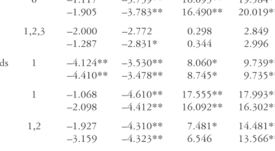
Table 3. Seasonal unit root test results. Lags t1 t2 F3 F23 F123 UK 0 –1.117 –3.739** 16.093** 19.584** 15.021** –1.905 –3.783** 16.490** 20.019** 15.895** Germany 1,2,3 –2.000 –2.772 0.298 2.849 3.226 –1.287 –2.831* 0.344 2.996 2.718 The Netherlands 1 –4.124** –3.530** 8.060* 9.739** 12.238** –4.410** –3.478** 8.745* 9.735** 13.070** Ireland 1 –1.068 –4.610** 17.555** 17.993** 13.810** –2.098 –4.412** 16.092** 16.302** 15.164** Portugal 1,2 –1.927 –4.310** 7.481* 14.481** 13.065** –3.159 –4.323** 6.546 13.566** 15.062** Spain 1,2,4 –1.035 –4.992** 30.785** 29.180** 21.916** –1.962 –5.091** 31.213** 29.964** 22.738**
Note: * and ** denote significance at the 5% and 1% significance levels, respectively. The order of
augmentation used in the HEGY test regression, in order to account for autocorrelation, is indicated in the column lags and results are presented for test regressions with seasonal dummies only (Dt) and with
seasonal dummies and a time trend (Dt + t). All tests were computed using Eviews 6. The column ‘Lags’
indicates the number of lags to guarantee the correction for autocorrelation.
We start this empirical section by looking at the non-stationary properties of the data, using for that purpose the seasonal unit root test proposed by Hylleberg et al (1990) [HEGY henceforth]. This preliminary investigation will allow us to establish the apparent degree of integration of the series at the seasonal and non-seasonal frequencies. This analysis will be complemented in the next section with the tests for persistence change.
Table 3 presents the results of the application of the HEGY seasonal unit root tests to the six quarterly time series under analysis. In performing the tests, auxiliary regressions with seasonal dummies only and seasonal dummies and a time trend were considered, as well as augmentation to correct for possible autocorrelation (the column ‘Lags’ indicates the number of lags found necessary in each case). The number of lags employed was determined using a general to specific lag selection strategy. For the purpose of analysis, the one-sided zero and Nyquist (biannual) frequency unit root t-statistics, t1 and t2, were considered. These statistics consider that under the null hypothesis there is a unit root, whereas under the alternative the series are stationary at these specific frequencies. Furthermore, joint test statistics to test for non-stationarity at the harmonic (annual) frequencies, F3, at all seasonal frequencies, F23, and at all frequencies, F123, were also used. The critical values used are shown in Table 4.
We observe from Table 3 that for the full sample with the exception of Germany, no seasonal unit roots can be found in the data, though all series with the exception of the Netherlands display a zero frequency (long-run) unit root, irrespective of whether seasonal dummies and a time trend or just seasonal dummies are considered in the regression. Next, we proceed by performing
Table 4. Critical values used. u τττττ 5% 1% 5% 1% t1 –2.82 –3.42 –3.37 –3.96 t2 –2.82 –3.42 –2.82 –3.42 F123 5.72 7.33 6.49 8.22 F23 6.03 8.01 6.00 7.95 F3 6.61 9.00 6.56 8.95
Note: u and τ indicate that seasonal dummies only and seasonal dummies and a time trend were considered in the test regression, respectively. These critical values were computed based on 50,000 replications.
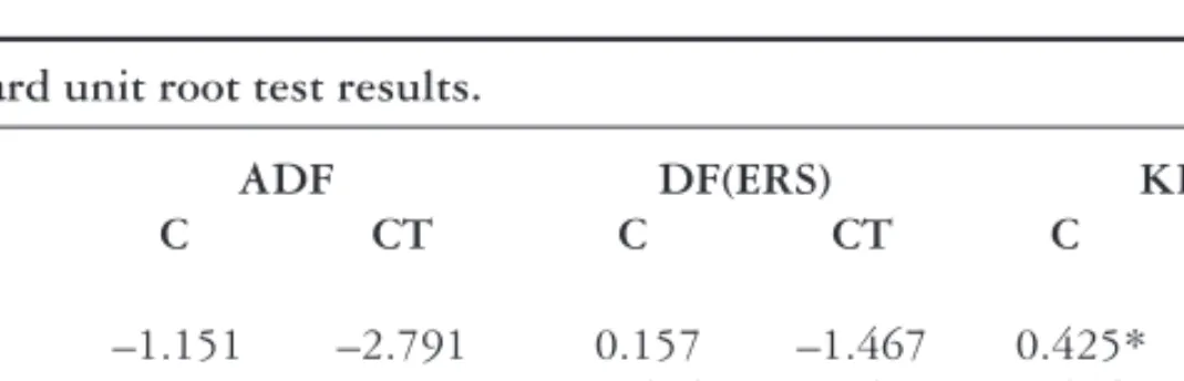
Table 5. Standard unit root test results.
ADF DF(ERS) KPSS Levels C CT C CT C CT UK –1.151 –2.791 0.157 –1.467 0.425* 0.081 Germany –1.509 –1.259 –0.684 –0.671 0.434* 0.401*** The Netherlands –2.445 –2.885 0.284 –1.006 0.715** 0.196** Ireland –1.139 –2.747 0.013 –1.626 1.201*** 0.069 Portugal –1.124 –3.099 2.378 0.743 0.789*** 0.071 Spain –0.097 –0.857 1.153 –0.966 1.285*** 0.124**
Note: *, ** and *** denote significance at the 10%, 5% and 1% significance levels, respectively. All
tests were computed using Eviews 6.
standard unit root tests at the zero frequency. The results of the augmented Dickey–Fuller test (ADF), the Elliott, Rothenberg and Stock’s recently proposed Dickey–Fuller type unit root test (DF-GLS) and the Kwiatkowski–Phillips– Schmidt–Shin test (KPSS) are displayed in Table 5. The results basically seem to confirm either the non-stationarity of the series in levels, that is the series are I(1) over the whole sample.
Persistence change evidence
To assess the validity of the persistence change hypothesis, we proceed by applying the tests described above, and the results are presented in Tables 6 and 7. Although the modified variants Kij, KRij and KMij have also been computed, they are not reported here as the results are of the same order of magnitude and therefore do not change the conclusions. Given the sample size, we considered the possibility of at most one change only in the order of integration. Using the critical values presented in Table 1 of Harvey et al (2006, p 451), the analysis in general indicates that all series present evidence of persistence change, although its direction is sometimes unclear. These are the cases for the tourism flows from the UK, Germany, Ireland and Spain. For these countries, the null hypothesis of I(0) is strongly rejected in favour of the I(0)–I(1) or
T
able 6.
Persistence change test results.
K 1 K 2 K 3 K R 1 K R 2 K R 3 K M 1 K M 2 K M 3 UK Dt 5.74** 15.54*** 38.89*** 32.90*** 80.23*** 167.60*** 32.90*** 80.23*** 167.60*** Dt + t 1.91 1.37 6.73* 1.19 0.77 3.85 1.91 1.37 6 .73 Germany Dt 0.80 0.77 7.03 12.19*** 33.27*** 74.06*** 12.19*** 33.27*** 74.06*** Dt + t 2.73* 8.89*** 25.71*** 58.64*** 272.94*** 553.82*** 58.64*** 272.94*** 553.82*** The Netherlands Dt 0.07 0.04 0.15 16.53*** 12.27*** 29.84*** 16.53*** 12.27** 29.84** Dt + t 0.73 0.63 4.84 7.63*** 25.45*** 57.58*** 7.63 25.45*** 57.58*** Ireland Dt 9.33*** 99.22*** 206.37*** 37.94*** 138.01*** 283.93*** 37.94 138.01*** 283.96*** Dt + t 1.13 0.72 3.90 2.44 2.37** 10.94** 2.44 2.37 10.94** Portugal Dt 1.11 1.06 6.86 25.04*** 72.63*** 152.55*** 25.04 72.63*** 152.55*** Dt + t 0.42 0.26 2.63 9.73*** 12.20*** 30.57*** 9.73 12.20*** 30.57*** Spain Dt 3.27 1.79 4.91 0.39 0.21 2.06 3.27 1.79 4 .91 Dt + t 4.27** 10.14*** 26.06*** 10.23*** 12.02*** 29.88*** 10.23 12.02*** 29.88*** Note : *
, ** and *** denote significance at the 10%, 5% and 1% significance levels, respectively
T
able 7.
Persistence change test results.
K1, J min K 2, J min K 3, J min K R 1, J min K R 2, J min K R 3, J min K M 1, J min K M 2, J min K M 3, J min UK Dt 5.65** 15.17*** 38.11*** 32.58*** 79.08*** 165.58*** 32.45*** 78.69*** 164.79*** Dt + t 1.91 1.37 6.70 1.18 0.75 3.76 1.88 1.33 6.56 Germany Dt 0.75 0.70 6.49 11.81*** 31.75*** 71.20*** 11.66*** 31.24*** 70.11*** Dt + t 2.72* 8.80*** 25.51*** 56.93*** 259.07*** 531.68*** 56.29*** 254.21*** 522.99*** The Netherlands Dt 0.07 0.03 0.13 16.08*** 11.78*** 28.83*** 15.90*** 11.61** 28.44** Dt + t 0.72 0.62 4.78 7.26*** 23.32*** 53.76*** 7.13*** 22.59*** 52.29*** Ireland Dt 9.14*** 96.33*** 201.33*** 37.44*** 135.34*** 279.34*** 37.24*** 134.43*** 277.56*** Dt + t 1.13 0.72 3.89 2.42* 2.34** 10.82** 2.41 2.33 10.77** Portugal Dt 1.07 1.02 6.61 24.51*** 70.37*** 148.55*** 24.30*** 69.61*** 147.02*** Dt + t 0.42 0.26 2.63 9.63*** 11.98*** 30.14*** 9.61*** 11.94*** 30.05*** Spain Dt 3.17 1.71 4.72 0.37 0.20 1.97 3.13 1.68 4.65 Dt + t 4.24** 9.97*** 25.72*** 10.02*** 11.61*** 29.07*** 9.95*** 11.46*** 28.74*** Note :
*, ** and *** denote significance at the 10%, 5% and 1% significance levels, respectively
I(1)–I(0) change. On the other hand, domestic tourism flows and flows from the Netherlands present evidence of a change from I(1) to I(0). In fact, the null hypothesis of I(0) is not rejected against the I(0)–I(1) change, but it is strongly rejected against the hypothesis of an I(1)–I(0) change. Hence, the analysis reveals statistically significant evidence that persistence has decreased in all countries. This decrease assumes a clearer pattern in the cases of Portugal and the Netherlands and a less clear direction in the remaining cases.
The results allow us to derive conclusions at two levels. First, the series show a persistence change from I(1) to I(0), which is symptomatic of a persistence decrease and a general trend towards a mean reverting behaviour. Second, it seems that the changes occur in the last years of the sample, in particular between 2000 and 2004, in all countries, implying that the results should be interpreted with some caution since the second subsample accounts for about 20 observations only.
EU membership has brought many benefits to Portugal by improving access to European policies and funds. The tourism sector is one of the fastest growing industries in the country (accounting for approximately 11% of GDP) and it has benefited strongly from EU integration, making Portugal one of the top destinations in the world. However, several events occurred in the period 2000– 2005 that definitely affected worldwide economies through the most sensitive sectors such as tourism. Nonetheless, the recent economic slowdown, coupled with phenomena of worldwide proportions (the terrorist attacks of 11 September and 4 March, the SARS outbreak and, most recently, the avian flu threat) have changed destination preferences and produced some substitution effects from which Portugal has benefited as a tourism destination.
Conclusion
This paper gathers evidence on persistence changes of tourism inflows from the UK, Germany, the Netherlands, Ireland, Portugal and Spain, measured by the number of overnight stays in hotel accommodation and similar establishments in the Algarve, one of the main tourism destinations in Portugal.
The central objective of this paper is an important issue for a country like Portugal, for two main interrelated reasons. First, the Portuguese economy relies heavily on tourism inflows, in particular the Algarve, the most prominent tourist region by excellence. Nevertheless, tourism inflows are also the basis of other regional economies as well. This has led to the development of research on the effects of tourism on economic performance at different levels: national, regional or even sectorial. The evidence of persistence change in tourism inflows brings a new challenge to empirical research and it will be at the centre of new developments regarding the role of the tourism industry worldwide.
The empirical results relied on the tests proposed by Kim (2000) and Harvey et al (2006), as the latter were particularly interesting in that they considered the null hypothesis to be I(0) or I(1) and allowed for breaks between periods of I(0) and I(1) under the alternative.
The preliminary analysis performed with the HEGY seasonal unit root tests detected a zero frequency non-stationary pattern in all series. The analysis that followed presented evidence of persistence change in the tourism inflows from
all countries considered in the sample. This means that tourism inflows to the Algarve are now less volatile than they were before and this may open the door for the definition of a global strategic plan towards the development of the sector in order to minimize the effects of seasonality and motivate tourists to return.
Although the identification of the reasons for this change is beyond the objective of this paper, we believe that the set of negative events that occurred at the beginning of this century, like the terrorist attacks and avian flu, may have contributed to the stabilization of tourism inflows, since there is evidence of positive destination substitution effects for Portugal, as documented in the literature (see, Andraz and Rodrigues, 2010). In fact, economic and social factors are usually mentioned as having direct effects on the willingness to travel to a foreign country. If economic instability with direct impact on people’s certainty about the future is determinant, the safety and political stability in the destination are also decisive factors. Portugal’s experience has been positive in terms of safety, as it has not experienced international or domestic security problems. Also, political stability has been a positive factor.
Furthermore, persistence change may be symptomatic of the positive effects generated by the adoption of the Euro as a common currency unit in most of the countries under analysis. Nevertheless, the analysis of the relative importance of these factors on tourism inflows to Portugal is far from being exhausted and will be explored in future research. Furthermore, the reduction of tourism volatility may also be a result of a long-term structural policy based on promoting the country and investment in tourism infrastructures and facilities, enacted by the Portuguese authorities with the purpose of attracting tourist loyalty and to make Portugal a preferential touristic destination. Of course, once this goal is achieved, government action will turn to short-run measures in order to minimize the effects of sudden shocks.
Finally, the results of this paper are not parochial with strict relevance for the Portuguese authorities. Tourism is a worldwide activity and several countries exhibit a structural dependency on this industry. Consequently, empirical research on tourism effects assumes a relevant position in the academic and political debate and a clear knowledge of its statistical properties is therefore required.
Endnotes
1. Results are omitted to save space but can be obtained from the authors on request.
References
Andraz, J., and Rodrigues, P. (2010), ‘Events that marked tourism to Portugal’, Applied Economic
Letters, forthcoming (http://www.tandf.co.uk/journals/titles/13504851.asp, accessed 11 February
2009).
Andrews, D.W.K (1993), ‘Tests for parameter instability and structural change with unknown change point’, Econometrica, Vol 61, pp 821–856.
Andrews, D.W.K., and Ploberger, W. (1994), ‘Optimal tests when a nuisance parameter is present only under the alternative’, Econometrica, Vol 62, pp 1383–1414.
Angeloni, I., Aucremanne, L., Ehrmann, M., Gali, J., Levin, A., and Smets, F. (2006), ‘New evidence on inflation persistence and price stickiness in the Euro area: implications for macro modelling’,
Journal of the European Economic Association, Vol 4, pp 562–574.
Busetti, F., and Taylor, A.M.R. (2004), ‘Tests of stationarity against a change in persistence’, Journal
of Econometrics, Vol 123, pp 33–66.
Davies, R.B. (1977), ‘Hypothesis testing when a nuisance parameter is present under the alternative’,
Biometrika, Vol 64, pp 247–254.
Dotsey, M., and King, R.G. (2006), ‘Pricing, production and persistence’, Journal of the European
Economic Association, Vol 4, No 5, pp 893–928.
Fuhrer, J.C., and Moore, G.R. (1995), ‘Inflation persistence’, Quarterly Journal of Economics, Vol 110, No 1, pp 127–159.
Galí, J., Gertler, M., and López-Salido, D. (2003), ‘Erratum to European inflation dynamics’,
European Economic Review, Vol 47, No 4, pp 759–760.
Gibson, H.D., and Lazaretou, S. (2001), ‘Leading inflation indicators for Greece’, Economic Modelling, Vol 18, pp 325–328.
Halunga, A.G., Osborn, D.R., and Sensier, M. (2009), ‘Changes in the order of integration of US and UK inflation’, Economics Letters, Vol 102, pp 30–32.
Hansen, B.E. (1991), ‘Tests for parameter instability in regressions with I(1) processes’, Journal of
Business and Economic Statistics, Vol 10, pp 321–335.
Harvey, D.I., Leybourne, S.J., and Taylor, A.M.R. (2006), ‘Modified tests for a change in persistence’,
Journal of Econometrics, Vol 134, pp 441–469.
Hylleberg, S., Engle, R.F., Granger, C.W.J., and Yoo, B.S. (1990), ‘Seasonal integration and cointegration’, Journal of Econometrics, Vol 44, pp 215–238.
Johnson, D.R. (2002), ‘The effect of inflation targeting on the behavior of expected inflation: evidence from an 11 country panel’, Journal of Monetary Economics, Vol 49, pp 1493–1519. Kim, J. (2000), ‘Detection of change in persistence of a linear time series’, Journal of Econometrics,
Vol 95, pp 97–116.
Kim, J.Y., Belaire Franch, J., and Badilli Amador, R. (2002), ‘Corringendum to detection of change in persistence of a linear time series’, Journal of Econometrics, Vol 109, pp 389–392.
Osborn, D.R. (1990), ‘A survey of seasonality in UK macroeconomic variables’, International Journal
of Forecasting, Vol 6, pp 327–336.
Park, J.Y. (1990), ‘Testing for unit roots and cointegration by variable addition’, in Fomby, T., and Rhodes, F., eds, Advances in Econometrics: Cointegration, Spurious Regressions and Unit Roots, Jai Press, London, pp 107–134.
Park, J.Y., and Choi, I. (1988), ‘A new approach to testing for a unit root’, Working Paper 88-23, Center for Analytic Economics, Cornell University, Ithaca, NY.
Phillips, P.C.B., and Perron, P. (1988), ‘Testing for a unit root in time series regression’, Biometrika, Vol 75, pp 335–346.
Phillips, P.C.B., and Xiao, Z. (1998), ‘A primer on unit root testing’, Journal of Economic Surveys, Vol 12, pp 423–470.
Steinsson, J. (2003), ‘Optimal monetary policy in an economy with inflation persistence’, Journal
of Monetary Economics, Vol 50, pp 1425–1456.
Vogelsang, T.J. (1998), ‘Trend function hypothesis testing in the presence of serial correlation’,