Class
Composition and
Student
Achievement:
Evidence from
Portugal
João Firmino
Luís Catela Nunes
Ana Balcão Reis
Carmo Seabra
Working Paper
# 624
1
Class Composition and Student Achievement. Evidence from Portugal.
João Firmino
a,1,*; Luis Catela Nunes
a,2; Ana Balcão Reis
a,3; Carmo Seabra
a,4aNova School of Business and Economics, Universidade Nova de Lisboa, Campus de Campolide, 1099-032, Lisbon, Portugal 1[email protected]; 2[email protected]; 3[email protected]; 4[email protected]
* Corresponding author at: Nova School of Business and Economics, Universidade Nova de Lisboa, Campus de
Campolide, 1099-032, Lisbon, Portugal. Tel.:+351 919010785
Abstract
We analyze the effects of several class compositional dimensions on individual student achievement. We make use of a rich dataset that allows tackling major endogeneity concerns stemming from non-random allocation of students between and within schools. We find that increasing the percentage of high achievers in a 6th grade class has a negative effect on student
performance, while in a 9th grade class the effect is in general non-significant. Students with no past retentions do better with
an increasing proportion of this same type of classmate. Larger shares of low-income classmates hurt performance in general. Apart from the past retention dimension in which there is evidence supporting students’ tracking, along all other compositional dimensions each class should reflect the respective school-grade population heterogeneity. Class composition rearrangements are estimated to provide a larger increment to performance than comparable reductions of class size.
Keywords: class composition; peer effects; student achievement
2
1
Introduction
In every educational system students are grouped into classes in schools. However, different agents within the education system may have different beliefs, interests, and constraints with respect to what might be considered an optimal placement of students across classes. Some parents may prefer to place their children among intellectually gifted classmates while others might prefer to place them in environments where specific cultural and social characteristics are predominant. Principals may have to comply with specific legislative conditions when setting up classes or may try to mirror different personal priors with respect to efficiency and fairness considerations.
One implicit difficulty stemming from the heterogeneity of views of what might be an optimal allocation of students across classes is the multitude of dimensions that characterize the composition of a class. Indeed, which dimension of class composition is the most important in explaining in-class behavior (and possibly the interactions between classmates outside the class) and consequently educational outcomes is a priori uncertain given the large number of dimensions that may be defined. Examples of such dimensions that have been studied in the literature are classmates’ previous attainment (Sund, 2009), gender and race (Hoxby, 2000a), or even language spoken (Yao, Ohinata, & Ours, 2016). On top of this, each class compositional dimension may affect educational outcomes heterogeneously depending on each student’s individual characteristics, which adds further complexity.
In this paper, and in contrast with most of the empirical literature, we analyze simultaneously the effects of several class compositional dimensions on individual student achievement. We make use of a rich dataset that allows us to tackle potential endogeneity problems resulting from non-random allocation of students between schools and across classes within each school. The dataset allows us to control for many student characteristics, including prior achievement, to measure several class composition dimensions, and also to control for heterogeneity across schools (using school fixed effects). We are also able to compute an instrumental variable that has been used in this literature – the school-grade average class size – to deal with possible contamination bias. In addition, the dataset includes information on 6th and 9th grade students so that
we can also study differences in the relevance of the class composition effects across different ages.
We address the following questions: 1) which dimensions of class composition affect an individual student achievement?; 2) do these effects depend on the students’ individual characteristics?; and 3) how do these results differ between 6th and 9th graders?
Our study is important from a public policy perspective since it offers a swift comparison of the direction and magnitude of the effects stemming from several dimensions of class composition. An evidence based comparison of different class compositional effects should help in the task of how to group students across classes.
This work is structured as follows. A literature review is provided in the next section. Section 3 details the dataset and presents some descriptive statistics. Section 4 specifies the econometric methodology. Section 5 presents the estimation results, while Section 6 discusses them. Section 7 summarizes policy implications for schools regarding class formation. Finally, Section 8 concludes.
3
2
Literature Review
This study places the class compositional effects’ identification within the education production function framework following, for example, Wößmann & West (2006), Todd & Wolpin (2003), Lazear (2001), Pritchett & Filmer (1999), Hanushek (1979), and Hanushek (1970). This approach may be traced back to the earlier Coleman Report (Coleman, Campbell, Hobson, McPartland, Mood, Weinfeld, et al., 1966) which presented the idea that educational outcomes were linked to a set of inputs that included the sort of peers one finds in school. Although it reported that the main predictors of educational outcomes were family and socio-economic background, the student body composition also helped to predict outcomes (especially those of minorities).
The type of schooling offered to students is influenced by school policies regarding class formation in at least two ways: how many and what kind of classmates exist in each class. Lazear (2001) formalizes the idea that for a given level of students’ quality (measured as the percentage of time each pays attention to the teacher) increasing class size would exponentially decrease class learning time – more students, more disruptions. One can similarly argue that for a given class size, increasing the proportion of disruptive students should also hamper overall classmates’ learning. These two similar arguments therefore establish an important link between class size and class composition, to which we will return below.
Concerning, specifically, the kind of classmates found in a given class, considerable attention has been devoted to the case where students are tracked into homogenous classes with respect to their ability or predetermined achievement levels. Sacerdote (2011) indicates that half of the surveyed research points to positive effects from this policy. However, this tends to be less clear when one allows for heterogeneous effects with respect to own students’ characteristics. For example, Burke & Sass (2013) provide evidence that different individuals (in terms of their own achievement level) seem to benefit differently from being placed in classes with higher shares of top, middle, or low achievers, which adds extra complexity to the effects of policies related with class quality homogeneity or heterogeneity.
More recent literature points to gains from having homogeneous classes according to past student performance (see Collins & Gan, 2013). In a randomized experiment in Kenyan schools, Duflo, Dupas, & Kremer (2011) report positive peer effects to the achievement levels of any type of student from the presence of high achievers in class. They further observe that sorting students to homogenous classes with respect to their initial levels of achievement caused all types of students to perform better. They explain that low achievers, although deprived of the potential contributions of the high achieving peers, might have benefited from better tailored teaching.
Some authors, e.g. Hanushek, Kain, Markman, & Rivkin (2003), Sund (2009), and Burke & Sass (2013), have been able to analyze longitudinal student-level datasets with students comparable to the ones we analyze in this paper, in terms of age and grade. The panel structure of the data allows them to control for several unobserved heterogeneities by including (separately or jointly) student, teacher, and school-by-grade fixed effects, or other combinations of these in their specifications. Hanushek et al. (2003) and Sund (2009) point to gains in achievement by the average student from having peers with higher levels of prior mean
4 achievement. Burke & Sass (2013), in turn, point to gains for a given student in having better, but not too much better, peers. They argue that a too large difference of prior achievement may hamper communication between students.
The consistent estimation of class composition effects requires endogeneity to be addressed. It arises from possible non-random sampling of students across schools and then across classes, see e.g. Wößmann & West (2006) and Bosworth (2014). Between-school sorting of students may occur, among other reasons, if parents are stratified regionally according to a given characteristic (e.g. professional occupation, level of education, or income). It causes a potential identification problem because the composition of the classes will then reflect the composition of the school which, in turn, is not independent of factors that determine, themselves, educational outcomes of the students (such as the parents’ characteristics). The correlation between school and class composition is not expected to be perfect, nevertheless, since students may be, in turn, sorted across classes, within-schools, in a systematic way. Within-school sorting may take the form of segregating low from high achievers, or segregating according to whether they have been retained in the past or not, perhaps reflecting different priors from principals or teachers related to how a class should be formed. Consequently, students may experience class compositions that might be predicted by their own characteristics, while these, in turn, are likely to explain their educational outcomes too.
To overcome endogeneity, different researchers have resorted to different approaches, conditional on the type of data at hand. Hoxby (2000a) exploits idiosyncratic variations (first differences) of gender and racial compositions in American schools, between adjacent years, due to unanticipated demographic changes, to avoid non-randomness allocation issues. She finds, first, that if the cohort average exam score increases by 1 point, then a student from that cohort scores 0.1 to 0.5 points more, on average; second, that, in a given cohort, a higher proportion of females leads to better performance in mathematics and reading for both males and females; finally, that peer effects are stronger and beneficial within racial groups.1 Hoxby
(2000b) finds no significant effects of class size on student achievement.2 She uses unexpected random
population variation as an instrument for class size while also applying school fixed effects.
There is a stream of literature that makes use of grade-school averages as instruments for class level variables. Akerhielm (1995) uses average class size across a given subject, within a school, to instrument actual class size. Although her procedure does account for within-school sorting, it does not take into account between-school sorting. Jürges & Schneider (2004), Wößmann & West (2006), and West & Wößmann (2006) also employ a two-stage regression procedure to identify class size effects (controlling for between-school sorting with school fixed effects) in the TIMSS’ database. They instrument actual class size with the average class size of the respective grade.
1 More recently, using a regression discontinuity design Card & Giuliano (2016) find that high achievers belonging to
ethnic minorities benefit from tracking to high achieving classes. Contrary to Hoxby (2000a), they hypothesize that there exists a harmful peer pressure within minorities, leading top achievers from minorities to underperform.
2 Although identification of class size effects is not the main goal of this paper, it is intimately related to class
5 Regarding within-school students’ allocation, West & Wößmann (2006) put forward the hypothesis of compensatory sorting. This hypothesis states that the class size reduction treatment comes hand in hand with a second treatment of sorting students with weak achievement-related inputs precisely to the classes of reduced dimensions. That is, students benefiting from less populated classes also experience, in general, a higher proportion of disadvantaged classmates (besides tending to be disadvantaged students themselves). They point out that countries with external exams are prone to induce such within-school compensatory schemes.3 The pressure to minimize the number of students with negative exam scores may dictate to a
certain extent how classes are formed every year.
From the above discussion of the literature we acknowledge two key points. First, the importance of including class size in the econometric specifications, at least as a control variable. One needs to hold constant the class size “treatment” when interpreting the class composition “treatments”. Or, in other words, controlling for class size is required for a ceteris paribus interpretation of the compositional coefficients (see Bosworth, 2014). Second, across econometric specifications that jointly include class compositional measures and class size, we may regard class size as the potential endogenous variable. This should be the case if those who are in charge, within each school, of class formation, believe that class size reduction is a stronger compensatory policy than specific class compositions. We provide suggestive evidence in favor of the class size compensatory hypothesis at the end of Section 3.
3
Data and Descriptive Statistics
The Portuguese educational system is divided into cycles.4 Within each cycle the composition of a
class is typically kept unchanged by schools. In particular, in the 2nd cycle (grades 5 and 6) students are
normally allocated to the same class, and in the 3rd cycle, the class composition is normally kept unchanged
from grades 7 to 9. A reorganization of the classes usually takes place when students move from the 6th to the
7th grade. At the end of each cycle students take compulsory national exams of reading and mathematics.
This paper makes use of an administrative dataset maintained by the Portuguese Ministry of Education.5 We use information on all students enrolled in public schools6, in continental Portugal, from
grades 6 and 9 in the academic year of 2011/2012. The dataset provides information on students’ class and school membership, their scores by subject and by type of examination, and their academic track. National exams’ scores of mathematics and reading taken at the end of the academic year provide the achievement measure (the dependent variable). These scores are recorded on a scale from 0 to 100 points. We also have information on previous achievement – baseline scores from national exams, which are measured on a scale
3 Which is the case of Portugal in the period studied.
4 The 1st cycle runs from grades 1 to 4, the 2nd cycle from grades 5 to 6, the 3rd cycle from grades 7 to 9, and the
secondary level from grades 10 to 12.
5 We thank DGEEC for providing access to the anonymized version of the MISI administrative dataset.
6 from 1 to 5 points.7 For 9th graders the baseline score refers to the 6th grade exam score, whereas for 6th
graders it refers to the 4th grade exam score.8
The dataset also includes several socio-demographic variables characterizing each individual student, such as gender, parents’ education (we use the education level of the parent with the highest degree), and home access to internet. By using the students’ birthdate, we created a dummy variable to distinguish those with no previous retentions from those with at least one. It takes the value one if the student’s age (at the beginning of the academic year – middle September of 2011) was equal to or lower than the reference age for the grade the student is enrolled in and zero otherwise. For 6th grade students the reference age is 12
years-old, while for 9th graders it is 15 years-old (the reference being the maximum age a student is expected
to have at the beginning of the academic year without having repeated any grade in past academic years). Cultural background is proxied by a dummy variable taking the value one if the student is a foreigner, i.e. if the student was born in one of the Portuguese speaking countries (excluding Portugal) and zero if born in Portugal.9 Low-income students were flagged if they received social support (by a dummy variable equal to
one if they did and zero otherwise).
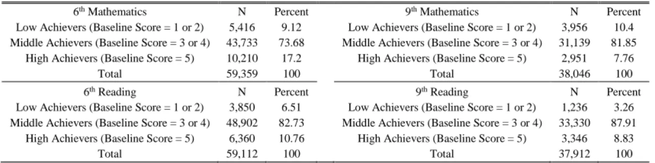
Our variables of interest related to the composition of the classes were created in the following manner. Knowing for each student his/her class membership, we were able to compute at the class level the percentage of: males, students with home access to internet, students with no previous retentions, students born in a foreign country, and low-income students. We further computed for each class the percentage of high and low achievers. We define as high achiever a student with a baseline score of 5 and as low achiever one with a baseline score of 1 or 2 (with the remaining cases composing the middle achievers). These groups, high and low achievers, vary from 3.3% to 17.2% of the respective relevant population, depending on subject and grade (see Table A.1 on Appendix A). We stress that all class compositional measures are “leave-out-percentages” as we excluded the contribution of student i when computing them.10 Thus, one
should interpret them as the percentage of classmates, of individual i, with a given characteristic, beyond individual i itself.
7 Grades are only available on a scale 1-100 since 2012.
8 National exam scores from 0 to 49 correspond to a negative evaluation while scores from 50 to 100 correspond to a
positive one. Baseline scores of 1 and 2 points correspond to a negative evaluation while 3, 4, and 5 points correspond to a positive evaluation. For students that repeated the 4th or the 6th grade, we use only their latest score as their baseline,
i.e. the one immediately before they progressed to the next grade.
9 The Portuguese speaking countries (excluding Portugal) are: Brazil, Angola, Cape Verde, Guinea-Bissau,
Mozambique, Sao Tome and Principe, and East Timor. The baseline case includes therefore students born in Portugal or in countries not belonging to Portuguese speaking countries. A third category differentiating those students born in neither Portugal nor a Portuguese speaking country would be of very small size and too heterogeneous.
10 Moreover, there are missing values with respect to baseline scores and place of birth for some students. We compute
these leave-out percentages by using only the non-missing information from a given class up to a maximum of 3 missing values. Students in classes with 4 or more missing values were dropped. Given a minimum class size of 14 it is unlikely that disregarding the contribution of up to 3 classmates would dramatically bias the true compositional measures for the classmates of those particular classes. Nevertheless, to control for such an effect, we considered three additional dummy variables that take the value of one if the pupil belongs to a class for which we bypassed missing information of 1, 2, or 3 classmates, respectively.
7 Finally, we created a measure of class age dispersion11 and calculated each student’s class size. The
dataset includes students enrolled in classes of extremely small size in relation to what was stipulated by law: a minimum and a maximum of 24 and 28, respectively. Although the law allowed for exceptional cases (e.g. to group students that would have exceeded the limits of the remaining classes), we considered only classes with at least 14 students. The number of students left out using this threshold is marginal.
We restrict our analysis to students enrolled under the regular academic track. This is the majority of the students in continental Portugal. DGEEC (2013, page 28) reports that in 2011-12, the percentage of students in public schools enrolled in the regular academic track in the 2nd and 3rd cycles were 99% and 90%,
respectively.
Finally, we only use students enrolled in schools with at least one class of both 6th and 9th grades
(which implies schools with at least two classes). This requirement ensures, first, that school fixed effects can be estimated (because each school will contribute with at least two classes to the estimation sample) and second, that the 1st stage of the instrumental variable procedure is also estimable (more details on this are
provided in Section 4).
The population of students that are used in our econometric analysis includes about 59,000 in the 6th
grade and about 38,000 in the 9th grade, corresponding to, respectively, 56.5% and 44.0% of the students
enrolled in the regular academic track in continental Portugal´s public schools, in the academic year 2011/2012.12 The fact that about half of the original population of students of each grade makes its way to
the final estimation sample is explained by the aforementioned set of restrictions imposed on the dataset and by missing data. The latter could introduce undesirable sample selection bias, but we argue that it should not be as large as one could a priori expect it to be.
There are three main different levels at which a missing value may have been generated: at the central, school, and individual level. The last level is mostly related with the fact that there is a non-marginal amount of missing values regarding parents’ education. This may happen either because students do not know the information or because parents fail to report it to the school. It is conceivable that students from more disadvantaged backgrounds may tend to be the ones that do not know such characteristics about their parents or, more likely, that their parents tend to show up less in school and are less likely to report the required information. This could lead to an under-representation of that kind of student in our regression samples and, in the limit, to an under-representation of classes composed mostly by them. We note that the inclusion of the individual students’ characteristics as regressors should control, to a large extent, for the likelihood of belonging to the regression sample. At the school level it may have happened that the administrative services of the schools failed to export information to the central authorities without random typos. Nevertheless, and regardless of its cause, the missing information originated at this level should be seen as school specific, thus captured by the school fixed effects included in the models. Lastly, losses of information that may have
11 The mean absolute deviation of the classmates’ age relative to the class average age. For instance, when this variable
takes the value 0.5 for a given class it means that each classmate’s age is on average half a year away from that class average age.
8 occurred at the central level should not be systematically related to students’ characteristics or, more important, to class composition.
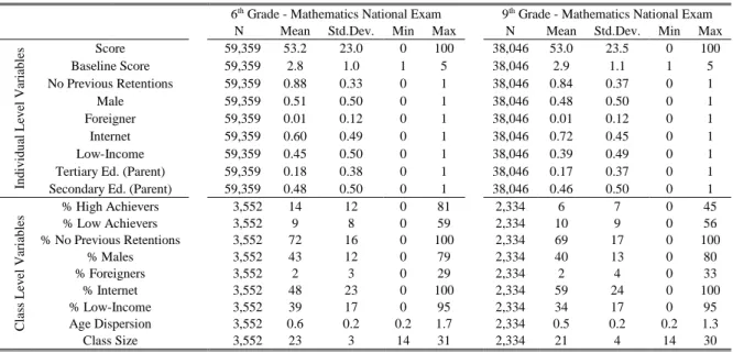
Some descriptive statistics of the final dataset are presented in Table 1.13 Regarding the statistics on
class level variables, note that the number of observations is the number of classes, not of students (hence the different number of observations for these variables). The distributions of the class level variables are shown in the Appendix in Figure A.1.
Table 1. Descriptive statistics.
6th Grade - Mathematics National Exam 9th Grade - Mathematics National Exam
N Mean Std.Dev. Min Max N Mean Std.Dev. Min Max
In d iv id u al Le v el V ar ia b le s Score 59,359 53.2 23.0 0 100 38,046 53.0 23.5 0 100 Baseline Score 59,359 2.8 1.0 1 5 38,046 2.9 1.1 1 5 No Previous Retentions 59,359 0.88 0.33 0 1 38,046 0.84 0.37 0 1 Male 59,359 0.51 0.50 0 1 38,046 0.48 0.50 0 1 Foreigner 59,359 0.01 0.12 0 1 38,046 0.01 0.12 0 1 Internet 59,359 0.60 0.49 0 1 38,046 0.72 0.45 0 1 Low-Income 59,359 0.45 0.50 0 1 38,046 0.39 0.49 0 1 Tertiary Ed. (Parent) 59,359 0.18 0.38 0 1 38,046 0.17 0.37 0 1 Secondary Ed. (Parent) 59,359 0.48 0.50 0 1 38,046 0.46 0.50 0 1
C la ss L ev el V ar ia b le s % High Achievers 3,552 14 12 0 81 2,334 6 7 0 45 % Low Achievers 3,552 9 8 0 59 2,334 10 9 0 56 % No Previous Retentions 3,552 72 16 0 100 2,334 69 17 0 100 % Males 3,552 43 12 0 79 2,334 40 13 0 80 % Foreigners 3,552 2 3 0 29 2,334 2 4 0 33 % Internet 3,552 48 23 0 100 2,334 59 24 0 100 % Low-Income 3,552 39 17 0 95 2,334 34 17 0 95 Age Dispersion 3,552 0.6 0.2 0.2 1.7 2,334 0.5 0.2 0.2 1.3 Class Size 3,552 23 3 14 31 2,334 21 4 14 30
We end this section observing suggestive evidence supporting the West & Wößmann (2006) hypothesis of compensatory within-school sorting along the class size dimension (see discussion in Section 2). The statistically significant unconditional correlations between class size and the class percentage of: high achievers, low achievers, students with no previous retentions, and low-income students are, respectively, 0.20, -0.14, 0.19, and -0.15. That is, we tend to find students with the a priori weakest achievement-related inputs (i.e. those in need of compensating inputs) in smaller classes.
4
Econometric Methodology
The benchmark model to estimate class composition effects is given by: 𝑌𝑖 = 𝛽0+ 𝑪𝒐𝒎𝒑𝒊,(−𝒊)′ 𝜷𝟏+ 𝑪𝒊′𝜷
𝟐+ 𝑿𝑖′𝜷𝟑+ 𝛾𝐺𝑖+ 𝑺𝑖′𝜶 + 𝜀𝑖 (1) where 𝑌𝑖 is the standardized mathematics or reading national exam score of student i; 𝑪𝒐𝒎𝒑𝒊,(−𝒊), 𝑪𝒊, 𝑿𝒊, 𝐺𝑖, and 𝑺𝒊 are explanatory variables; 𝜀𝑖 is the student i idiosyncratic error term, and 𝛽0, 𝜷𝟏, 𝜷𝟐, 𝜷𝟑, 𝛾, and 𝜶 are parameters to be estimated. Although the explanatory variables are indexed at the student i level, they are calculated at specific individual, class, or school levels as explained next.
13 These statistics refer to students with a mathematics national exam score. Table A.2 in the Appendix presents the
same statistics for those with a reading national exam score. Both populations are very similar: they differ by only a few hundred.
9 𝑪𝒐𝒎𝒑𝒊,(−𝒊) is the vector containing the percentages of classmates of student i with a given characteristic – high achievers, low achievers, no previous retentions, males, born in a foreign country, home access to internet, and low-income. These are the class compositional variables of interest for this paper. Recall from Section 3 that these compositional measures were computed in a leave-out fashion and based on
predetermined characteristics of the students. The former enables them to be interpreted as peer measures,
while the latter avoids reflexivity bias.14
The 𝑺𝒊 vector includes school dummy variables, i.e. school fixed effects. As discussed in Section 2, consistent estimation of 𝜷𝟏 requires that we credibly control for endogeneity stemming from non-random allocation of students between and within schools. One popular way in the literature to control for between-school sorting is to include between-school fixed effects. These control for anything that is between-school specific, namely the type and number of students that it attracts, but also school specific policies with respect to class formation. In turn, these and other school specificities may well impact student outcomes, making their omission a source of bias. Including school fixed effects helps to interpret the estimated 𝜷𝟏 as if students had been randomly allocated across schools. Further, school fixed effects can also be seen as a step to control for teacher between-school sorting under similar arguments.
Next, 𝑿𝒊 is the vector containing all the individual level characteristics of the students that were presented in Section 3.15 The inclusion of these variables is important in order to control for within-school
sorting. In fact, as discussed in the literature review, educational systems with external exams (the case of Portugal) induce compensatory policies within the schools (i.e. within-school sorting of students). Given the suggestive evidence presented in Section 3 that students with weaker inputs tend to be found alongside each other (in smaller classes), we consider that, indeed, those authorities are likely to have taken into account the students’ characteristics during the class formation process, at least to some extent. On top of this, the information that school authorities have at the moment of class formation is mostly based on the administrative dataset we actually use in this study. In addition, we stress the inclusion within vector 𝑿𝒊 of the baseline score as a control variable. Its inclusion allows us to control for possible correlations between contemporary class assignment and past factors.16 Thus, conditional on the set of individual students’
characteristics, one is closer to interpret the estimated 𝜷𝟏 as if students had been randomly allocated across
classes within schools.17
14 Such a bias would occur if, for example, the percentages of high or low achievers had been defined through the
outcome score and not by the predetermined baseline score, as we did. In that case we would then have the outcome of student i influencing his/her classmates’ outcome and vice-versa, thereby creating a reflection bias (see Hanushek et al., 2003).
15 Dummy variables describing each student baseline score, parents’ education, previous retention status, gender,
foreign background status, internet at home status, and low-income status.
16 Todd & Wolpin (2003) and Hanushek & Rivkin (2010) provide theoretical frameworks that justify the use of a
baseline score as a summary of past factors under some technical assumptions.
17 Inclusion of parents’ education, besides capturing its direct effect as an input on students’ achievement, should help
to control for both between-school and within-school sorting since it may be positively related with parents’ ability and willingness to place their children in the “best” school and then to informally bargain within the school for the “best” class.
10 The term 𝑪𝒊 is a vector containing other class level control variables, such as class size, age dispersion in the class, and dummies flagging classes with 1, 2, or 3 classmates whose information was not used when computing the class compositional variables of interest because of missing data. As discussed in the literature review, one needs to control for class size as this is a possible confounding treatment that seems to go hand in hand with the class compositional treatments. Moreover, its inclusion contributes to a clearer
ceteris paribus interpretation of the relevant coefficients. Inclusion of the dummies related with missing
information at the class level aims at controlling for any unobserved features of such classes that might explain why that information is missing. If those unobserved features somehow relate with student outcomes then not controlling for them could bias the estimate of 𝜷𝟏. Lastly, controlling for class age dispersion means that one is closer to interpret the marginal effects of the different class compositions as if behaviors stemming from dispersion of ages at the class level were fixed. So, for example, the marginal effect of a change in the percentage of students with no previous retentions captures the effects stemming from a change in the structure of peers’ past academic experience, instead of the peer effects stemming from changing the class age structure (which is being held fixed).18
Finally, 𝐺𝑖 is a grade dummy variable that accounts for possible grade specific features correlated with both the students’ outcomes and the composition of the classes in a given grade.
To allow the marginal effects of the class compositional variables to be heterogeneous according to students’ individual characteristics we consider an alternative model allowing for interactions between each class composition variable and the corresponding individual characteristic. More precisely, we specify the model as: 𝑌𝑖 = 𝛽0+ [%𝐻𝑖𝑔ℎ 𝐴𝑐ℎ𝑖𝑒𝑣𝑒𝑟𝑠𝑖,(−𝑖)× 𝕀𝐿𝑜𝑤 𝐴𝑐ℎ𝑖𝑒𝑣𝑒𝑟𝑖=1]𝛽1 %𝐻×𝐿𝑜𝑤+ [%𝐻𝑖𝑔ℎ 𝐴𝑐ℎ𝑖𝑒𝑣𝑒𝑟𝑠𝑖,(−𝑖)× 𝕀𝑀𝑖𝑑 𝐴𝑐ℎ𝑖𝑒𝑣𝑒𝑟𝑖=1]𝛽1 %𝐻×𝑀𝑖𝑑+ [%𝐻𝑖𝑔ℎ 𝐴𝑐ℎ𝑖𝑒𝑣𝑒𝑟𝑠𝑖,(−𝑖)× 𝕀𝐻𝑖𝑔ℎ 𝐴𝑐ℎ𝑖𝑒𝑣𝑒𝑟𝑖=1]𝛽1 𝐻%×𝐻𝑖𝑔ℎ+ [%𝐿𝑜𝑤 𝐴𝑐ℎ𝑖𝑒𝑣𝑒𝑟𝑠𝑖,(−𝑖)× 𝕀𝐿𝑜𝑤 𝐴𝑐ℎ𝑖𝑒𝑣𝑒𝑟𝑖=1]𝛽1 %𝐿×𝐿𝑜𝑤+ [%𝐿𝑜𝑤 𝐴𝑐ℎ𝑖𝑒𝑣𝑒𝑟𝑠𝑖,(−𝑖)× 𝕀𝑀𝑖𝑑 𝐴𝑐ℎ𝑖𝑒𝑣𝑒𝑟𝑖=1]𝛽1 %𝐿×𝑀𝑖𝑑+ [%𝐿𝑜𝑤 𝐴𝑐ℎ𝑖𝑒𝑣𝑒𝑟𝑠𝑖,(−𝑖)× 𝕀𝐻𝑖𝑔ℎ 𝐴𝑐ℎ𝑖𝑒𝑣𝑒𝑟𝑖=1]𝛽1 %𝐿×𝐻𝑖𝑔ℎ [%𝑁𝑜 𝑃𝑟𝑒𝑣𝑖𝑜𝑢𝑠 𝑅𝑒𝑡𝑒𝑛𝑡𝑖𝑜𝑛𝑠𝑖,(−𝑖)× 𝕀𝑁𝑜 𝑃𝑟𝑒𝑣𝑖𝑜𝑢𝑠 𝑅𝑒𝑡𝑒𝑛𝑡𝑖𝑜𝑛𝑠𝑖=1]𝛽1 𝑁𝑜 𝑅𝑒𝑡𝑒𝑛𝑡𝑖𝑜𝑛𝑠+ [%𝑁𝑜 𝑃𝑟𝑒𝑣𝑖𝑜𝑢𝑠 𝑅𝑒𝑡𝑒𝑛𝑡𝑖𝑜𝑛𝑠𝑖,(−𝑖)× 𝕀𝐴𝑡 𝐿𝑒𝑎𝑠𝑡 1 𝑃𝑟𝑒𝑣𝑖𝑜𝑢𝑠 𝑅𝑒𝑡𝑒𝑛𝑡𝑖𝑜𝑛𝑖=1]𝛽1𝐴𝑡 𝐿𝑒𝑎𝑠𝑡 1 𝑅𝑒𝑡𝑒𝑛𝑡𝑖𝑜𝑛+ [%𝑀𝑎𝑙𝑒𝑠𝑖,(−𝑖)× 𝕀𝑀𝑎𝑙𝑒𝑖=1]𝛽1𝑀𝑎𝑙𝑒+ [%𝑀𝑎𝑙𝑒𝑠𝑖,(−𝑖)× 𝕀𝐹𝑒𝑚𝑎𝑙𝑒𝑖=1]𝛽1𝐹𝑒𝑚𝑎𝑙𝑒+ [%𝐹𝑜𝑟𝑒𝑖𝑔𝑛𝑒𝑟𝑠𝑖,(−𝑖)× 𝕀𝐹𝑜𝑟𝑒𝑖𝑔𝑛𝑒𝑟𝑖=1]𝛽1 𝐹𝑜𝑟𝑒𝑖𝑔𝑛𝑒𝑟+
18 As the percentage of students with no previous retentions increases, on average the class age dispersion also
decreases. Nevertheless, this is not a one-to-one relationship. Some classes have a relatively high age dispersion but with few students with at least one retention (e.g. classes with students that entered the education system very early – 5 years old – alongside other students that entered it when they were almost 7 years-old; and both groups never repeated a grade). On the other hand, there are classes with many students with at least one previous grade retention whose ages are aligned, i.e. with a relatively small class age dispersion.
11 [%𝐹𝑜𝑟𝑒𝑖𝑔𝑛𝑒𝑟𝑠𝑖,(−𝑖)× 𝕀𝑁𝑜𝑛 𝐹𝑜𝑟𝑒𝑖𝑔𝑛𝑒𝑟𝑖=1]𝛽1𝑁𝑜𝑛 𝐹𝑜𝑟𝑒𝑖𝑔𝑛𝑒𝑟+ [%𝐼𝑛𝑡𝑒𝑟𝑛𝑒𝑡𝑖,(−𝑖)× 𝕀𝐼𝑛𝑡𝑒𝑟𝑛𝑒𝑡𝑖=1]𝛽1𝐼𝑛𝑡𝑒𝑟𝑛𝑒𝑡+ [%𝐼𝑛𝑡𝑒𝑟𝑛𝑒𝑡𝑖,(−𝑖)× 𝕀𝑁𝑜 𝐼𝑛𝑡𝑒𝑟𝑛𝑒𝑡𝑖=1]𝛽1𝑁𝑜 𝐼𝑛𝑡𝑒𝑟𝑛𝑒𝑡+ [%𝐿𝑜𝑤 𝐼𝑛𝑐𝑜𝑚𝑒𝑖,(−𝑖)× 𝕀𝐿𝑜𝑤 𝐼𝑛𝑐𝑜𝑚𝑒𝑖=1]𝛽1𝐿𝑜𝑤 𝐼𝑛𝑐𝑜𝑚𝑒+ [%𝐿𝑜𝑤 𝐼𝑛𝑐𝑜𝑚𝑒𝑖,(−𝑖)× 𝕀𝑁𝑜𝑛 𝐿𝑜𝑤 𝐼𝑛𝑐𝑜𝑚𝑒𝑖=1]𝛽1𝑁𝑜𝑛 𝐿𝑜𝑤 𝐼𝑛𝑐𝑜𝑚𝑒+ 𝑪𝒊′𝜷𝟐+ 𝑿′𝑖𝜷𝟑+ 𝛾𝐺𝑖+ 𝑺𝑖′𝜶 + 𝜀𝑖
or more compactly by: 𝑌𝑖 = 𝛽0+ [𝑪𝒐𝒎𝒑𝒊,(−𝒊)′ × 𝕀 𝑿𝒊=𝟏]𝜷𝟏 𝑿𝒊=𝟏+ [𝑪𝒐𝒎𝒑 𝒊,(−𝒊) ′ × 𝕀 𝑿𝒊=𝟎]𝜷𝟏 𝑿𝒊=𝟎+ 𝑪𝒊′𝜷𝟐+ 𝑿𝑖′𝜷𝟑+ 𝛾𝐺𝑖+ 𝑺𝑖′𝜶 + 𝜀𝑖 (2) where 𝕀 denotes the indicator function. That is, we assess how a (leave-out) percentage of a given type of student in a class (i.e. 𝑪𝒐𝒎𝒑𝒊,(−𝒊)) affects the student of that type and the student of the other type. For example, in this model, the class (leave-out) percentage of males may impact male and female students differently.
The models in equations (1) and (2) rely on numerous control variables offered by our dataset to reduce possible endogeneity biases that could plague the estimates of the true class compositional effects. However, given what was argued in Section 2 and given the suggestive evidence shown in Section 3, we consider that there is the chance for class size to be the within-school driver of endogeneity. In such case, an ordinary least squares (OLS) estimation of the previous models may still result in biased estimates despite the many controls used in the regressions. Hence, we also estimate the model in equation (2) using an instrumental variables (IV) approach. Class size is instrumented with school-grade average class size following Jürges & Schneider (2004), Wößmann & West (2006), and West & Wößmann (2006). We employ this IV estimation as a robustness check. If the class compositional variables correlate with the possibly endogenous class size variable (which they somewhat do) then the possible endogeneity of the latter may affect the correct estimation of the effects of the former.
Regarding the two necessary requirements for this instrument to hold valid, we can say that, on one hand, grade-school average class size must be correlated with the actual class sizes that compose that grade in a given school. After all, even though schools may sort weaker students to shorter classes in a given grade, it must be the case that schools that have relatively more students must sort them to shorter classes that are relatively more populated than shorter classes of less populated grades-schools. Given that schools must obey certain national rules regarding class formation and face, at each academic year and for each grade, specific cohorts with a given size, then, conditional on additive grade and school fixed effects (the latter capturing school specific rules or resources correlated with the number of classes opened and school specific levels of enrolment), variations in the grade-school average class size should reflect exogenous demographic variations of the respective cohort in the area of influence of the school. On the other hand, as stated by Wößmann & West (2006), the exclusion condition of the instrument is likely to hold too: “There is also no
12
reason to expect that the average class size would affect the performance of students in a specific class in any other way than through its effect on the actual size of the class of the students.” (p. 700).
The first stage of the IV estimation is to estimate the following equation predicting 𝐶𝑆𝑖, the class size for each individual i:
𝐶𝑆𝑖 = 𝑏0+ [𝑪𝒐𝒎𝒑𝒊,(−𝒊)′ ∗ 𝕀𝑿𝒊=𝟏]𝒃𝟏 𝑿𝒊=𝟏+ [𝑪𝒐𝒎𝒑 𝒊,(−𝒊) ′ ∗ 𝕀 𝑿𝒊=𝟎]𝒃𝟏 𝑿𝒊=𝟎+ 𝑪 𝒊 ′𝒃 𝟐+ 𝑏𝐶𝑆̅̅̅̅𝐶𝑆̅̅̅̅𝑖+ 𝑿𝑖′𝒃𝟑+ 𝑔𝐺𝑖+ 𝑺𝑖′𝒂 + 𝑒𝑖 (3) with 𝐶𝑆̅̅̅̅𝑖 representing the (excluded) instrument – student’s i school-grade average class size. Note that to avoid perfect collinearity between the instrument and the school fixed effects in this first stage regression, one has to pool both 6th and 9th grades and ensure that each school “contributes” with at least two classes –
one class from each of the two grades. As explained in Section 3, we have already imposed this requirement on the dataset.
A comparison of the OLS and IV estimation results for model (2), detailed in the next section, provides evidence of no significant differences of the class compositional coefficients between them. We take this as evidence that the OLS version delivers estimates of the class compositional effects free of endogeneity contamination bias stemming from the possibly endogenous class size variable. We thus proceed with the OLS estimation of model (2) for 6th and 9th graders separately, with the intention of
uncovering possible differences in the class compositional effects for different ages.
5
Estimation Results
5.1 Results pooling grades 6 and 9
Table 2 provides for both measures of achievement mathematics and reading the OLS estimation results of the model in equation (1) above. Column (1) presents the results of a simple specification of model (1), in which only student between-school sorting is controlled for (via school fixed effects), and only two class compositional variables – (leave-out) percentage of high and low achievers – are included along with class size. These two compositional measures are the ones that relate more closely to what the literature defines as class student “quality”. Then, column (2) adds the full set of individual student level controls that aim to account for student within-school sorting. The final column (3) adds the remaining class compositional measures, which further alleviate possible confounding treatment effects, thus improving the
ceteris paribus interpretation of each of the estimated compositional coefficients.
Indeed, the coefficients attached to the proportion of high and low achievers have significant changes (both in sign and magnitude) as each set of control and treatment variables are consecutively added. In turn, the estimated effect of class size changes from statistically significant and positive to non-significant.
In Table 3, column (1) we present the results when we allow for heterogeneous class compositional marginal effects, corresponding to the model in equation (2). The picture does not change considerably regarding the non-significant effect of class size. Overall, these changes demonstrate the importance of controlling for within-school sorting of students and for possible confounding treatment effects, which improve the causal interpretation of the class compositional effects.
13
Table 2 Estimation results using as outcomes the national exam scores in Mathematics and Reading
Explanatory Variables
Pooled 6th and 9th Graders
OLS
(1) (2) (3)
Mathematics Reading Mathematics Reading Mathematics Reading % High Achievers 0.0080*** 0.0110*** -0.0026*** 0.0005 -0.0045*** -0.0015*** % Low Achievers -0.0078*** -0.0073*** -0.0005 -0.0014** 0.0013** 0.0003 % No Previous Retentions -- -- -- -- 0.0027*** 0.0021*** % Males -- -- -- -- 0.0001 -0.0005 % Foreigners -- -- -- -- -0.0010 -0.0031** % Internet -- -- -- -- 0.0009*** 0.0007*** % Low-Income -- -- -- -- -0.0033*** -0.0023*** Age Dispersion -- -- -- -- -0.087*** -0.050* Class Size 0.017*** 0.017*** 0.006*** 0.004*** 0.002 0.001 No Previous Retentions -- -- 0.42*** 0.37*** 0.41*** 0.37*** Male -- -- -0.08*** -0.22*** -0.08*** -0.22*** Foreigner -- -- -0.05** -0.06*** -0.05*** -0.06*** Internet -- -- 0.10*** 0.08*** 0.10*** 0.08*** Low-Income -- -- -0.14*** -0.11*** -0.14*** -0.10*** Baseline Score Dummies -- -- Parent Education Dummies -- -- Grade Fixed Effects School Fixed Effects Adjusted R2 9.8% 7.1% 49.7% 43.9% 50.0% 44.1%
N 112,417 111,961 99,899 99,562 97,405 97,024 Notes: Significance levels: * p<.10, ** p<.05, *** p<.01. Robust standard errors clustered at the class level. Each outcome variable was standardized to have mean zero and std. dev. of one. Each model also contains dummies equal to 1 if student i peers' measures were computed using partial class information, i.e. if one, two, or three classmates of i had missing information about their baseline scores or their place of birth. The class composition variables (i.e. the percentages of classmates of student i with a given characteristic) were computed in a leave-out fashion, i.e. excluding student i. Each model contains an intercept and pools students from grades 6 and 9. Only classes with 14 or more students were used and they had to belong to schools with at least one class of grade 6 and, simultaneously, another of grade 9 (i.e. each school contributed with at least two classes).
One would expect the class size effect to be detectable once sorting of students and confounding class level treatments are taken into account. Nevertheless, we do not observe it. In reality, the class size effect may not exist as obtained by Hoxby (2000b) or, if it does, it may be small in magnitude (Bosworth, 2014). Or it may be necessary to record greater class size variation in absolute terms (greater than from 14 to 31 students as we observe in our data) to capture a significant effect, as in Duflo, Dupas, & Kremer (2015) (they observe classes halving from 80 to 40 students). It may, however, also mean that the class size coefficient may still be plagued by endogeneity bias. Recall that, as discussed in Section 4, this may cause the class compositional coefficients – the ones of interest for this paper – to also be biased, which, coupled with the suspicion that class size is the within-school driver of endogeneity, justifies our choice to be conservative. The use of the IV estimator to estimate equation (2) provides then a robustness check against this possibility. Before presenting the IV estimation results, we discuss, next, two points worthy of mention regarding the results of the first stage of the corresponding 2SLS procedure (see Table A.3 in the Appendix).
First, many of the individual and class compositional variables are significant at predicting class size, at least at the 5% level. This reinforces the idea that, indeed, the class size each student experiences might be determined by his/her own characteristics (via purposeful within-school sorting). It also confirms that at least some of the class compositional treatments are, in fact, related to class size. Hence, it is advisable to jointly include them in the educational production function.
Second, and more importantly, the (excluded) instrument – grade-school average class size – significantly predicts class size (at the 1% level) even when conditioning on all controls as well as on grade and school fixed effects. This means that the instrument should account for grade-by-school heterogeneity, e.g. exogenous variation on the size of 6th and 9th graders’ cohorts around the influence area of the school,
14 that might not otherwise be picked up by additive school and grade fixed effects. In turn, the usual first stage F-statistic testing the significance of the excluded instrument is well above the rule of thumb of 10, and the instrument is therefore not weak.
The IV estimation results are shown in column (2) of Table 3. The signs and magnitudes of the estimated coefficients are quite similar to those obtained by OLS in column (1). The exceptions are mild changes in the coefficients of class size and class age dispersion for the reading specification which become negative and significant at the 5% and 10% levels, respectively. The change in the class size coefficient is expectable assuming that class size may still be plagued, to some degree, by endogeneity, and that the instrument is valid.19 We conduct a Durbin-Wu-Hausman test to formally assess if, under the hypothesis that
the instrument is valid, there is evidence of endogeneity, i.e. that the estimates of the 2SLS are statistically significantly different from those obtained by OLS. This test is presented at the bottom of Table A.3. For mathematics we fail to reject the null hypothesis of exogeneity, whereas for reading we reject it at the 1% level of significance.20 All in all, there is no evidence that possible endogeneity of class size, especially with
respect to the reading specification, is contaminating the estimates of the class compositional variables in column (1) of Table 3. None of the compositional estimates change considerably whether instrumenting class size or not. We then conclude that the estimation results of the model in equation (2) are reliable causal estimates of the class composition effects.
5.2 Results separating grades 6 and 9
The estimation results of the model in equation (2) applied separately to the populations of grades 6 and 9 are presented in Table 3, columns (3) and (4), respectively. We assume that the evidence in favor of the no endogeneity contamination bias provided by the comparison of the pooled estimates of columns (1) and (2) of Table 3 extends to the 6th and 9th grades’ estimates of columns (3) and (4) since, as explained
above, the IV procedure cannot be implemented when estimating separate models for each of the grades.
5.2.1 6th Grade
The results suggest that a given 6th grader is harmed when facing a higher percentage of high achievers
in his/her class. This negative effect increases in magnitude as that given 6th grade student is a better
performer (i.e. as his/her baseline score is higher), see column (3) of Table 3. An increase of 20 percentage points (p.p.) of high achievers in his/her class (about four more high achievers and four fewer middle
19 This result, at first sight, differs from Wößmann & West (2006) who, using the TIMSS database, find that class size,
for Portuguese students, has a significant positive coefficient on mathematics. However, the fact that our estimate for class size with respect to the math specification started as significantly positive in the simplest model in column (1) of Table 2, and then turned non-significant in column (2) of Table 3, comes in line with their overall results. As they include school fixed effects and instrument class size with school-grade average class size they also observe the same general movement of the class size coefficient: from significant positive to non-significant and from non-significant to significant negative.
20 Since reading and mathematics are taught to the same class these results suggest that the structural effect of class size
differs across subjects. That is, across subjects there may be considerable differences in the way the same input impacts the corresponding achievement level. In this case it may be that smaller classes are relatively more incremental to reading than to mathematics. Students may be more dependent on what is discussed in-class in reading as it may be a subject of a more communicative nature and suffer more with larger and more disruptive classes.
15 achievers in a class of size 20)leads to a loss in performance, in mathematics, of 5%,21 8%, and 10.8% of a
SD, depending on whether the student is a low, middle, or high performer, respectively. For reading the respective values are 0% (not significant), 4%, and 5.6% of a SD; hence the same pattern is observed.
In turn, the percentage of low achievers delivers opposite results, in general. An increase of low achievers leads to a statistically significant gain in mathematics performance around 4% to 5% of a SD, whether the student is a low, middle, or high performer in the 6th grade. On the other hand, looking at the
reading specification, a positive variation in the proportion of low achievers negatively affects those 6th
graders that are themselves low achievers. It translates into a loss of about 8% of a SD. The increment of the percentage of low achievers produces a gain for middle and high achievers of about 2.8% and 9.4% of a SD, respectively.
The impact of increasing the percentage of classmates with no previous retentions is to increase the achievement of 6th graders that have no previous retentions by a percentage ranging from 5.2% to 7.4% of a
SD, depending on the subject we look at. There is no statistical evidence of students with at least one retention in their past schooling trajectory being affected by the proportion of students with at least one previous retention.
The impact of the percentage of males across 6th grade classes is insignificant in most cases. Only for
males in math is there a small and positive significant effect (2.2% of a SD) from increasing it.
As in the previous case we observe only one particular significant effect regarding the impact of the class percentage of foreigners on 6th grade achievement. It is found on the reading specification: 6th grade
foreigners are harmed by larger shares of foreign classmates. This effect is around 4.5% of a SD given an increase of 5 p.p. in the percentage of students born abroad.22
One can notice, as well, that positively varying the proportion of students with home access to the internet, in a given class, seems to positively (but weakly) affect 6th grade students. The gain in having more
classmates with internet varies from 1.6% to 3% of a SD, depending on the subject and on whether the student has internet at home or not.
Finally, 6th graders seem to be hurt with larger shares of low-income classmates. Increasing the
proportion of low-income students, in a given 6th grade class hampers the performance of a given
low-income student from that class by about 5.3% of a SD, in both subjects; and that of a given non-low-low-income student from that class by 5% to 9.2% of a SD, depending on the subject.
21 This value results from multiplying by 20 p.p. the respective estimate of the marginal effect of the class
compositional variable (which is measured inpercentage points). In this case the decrease in 5% of a SD is obtained by multiplying by 20 p.p the estimated marginal effect of -0.0025 (of a SD). Note that all the remaining effects presented in this section and subsequent ones refer to a 20 p.p. variation in the relevant explanatory variable, unless otherwise stated.
22 Although a 20 p.p. variation in the proportion of foreign born students in a given class is within its observed variation
(on both grades) it is still quite large compared to its standard deviation. Increasing the percentage of foreign born students in a given class by 5 p.p. is closer to its standard deviation (see Table 1).
16
Table 3 Estimation results using as outcomes the national exam scores in Mathematics and Reading
Explanatory Variables
Pooled 6th and 9th Graders 6th Graders 9th Graders
OLS IV (2nd Stage) OLS OLS
(1) (2) (3) (4)
Mathematics Reading Mathematics Reading Mathematics Reading Mathematics Reading % High Achievers ×
{
Low Achiever -0.0024*** -0.0023 -0.0024*** -0.0022 -0.0025** -0.0018 -0.0008 -0.0014 Middle Achiever -0.0041*** -0.0011** -0.0041*** -0.0010* -0.0040*** -0.0020*** 0.0020** 0.0010 High Achiever -0.0064*** -0.0033*** -0.0064*** -0.0033*** -0.0054*** -0.0028*** 0.0003 -0.0017 % Low Achievers ×{
Low Achiever 0.0016** -0.0048*** 0.0016** -0.0051*** 0.0026** -0.0040** -0.0009 -0.0071 Middle Achiever 0.0012** 0.0008 0.0011** 0.0006 0.0021*** 0.0014* -0.0025*** -0.0000 High Achiever 0.0029*** 0.0003 0.0029*** -0.0001 0.0024* 0.0047*** 0.0020 0.0033 % No Previous Retentions ×{
No Previous Retentions 0.0035*** 0.0029*** 0.0035*** 0.0031*** 0.0037*** 0.0026*** 0.0025*** 0.0038***At Least 1 Previous Retention -0.0006 -0.0003 -0.0005 -0.0001 -0.0011 -0.0008 -0.0008 0.0010 % Males ×
{
Male 0.0005 0.0002 0.0005 0.0002 0.0011** 0.0001 0.0003 0.0011* Female -0.0003 -0.0011*** -0.0003 -0.0011*** 0.0001 -0.0007 -0.0001 -0.0005 % Foreigners ×{
Foreigner 0.0037 -0.0077** 0.0037 -0.0076** 0.0047 -0.0090** 0.0066 -0.0032 Non-Foreigner -0.0012 -0.0030** -0.0012 -0.0031** 0.0004 -0.0007 -0.0007 -0.0036** % Internet ×{
Internet 0.0011*** 0.0006** 0.0011*** 0.0007** 0.0015*** 0.0013*** 0.0007 0.0004 No Internet 0.0005 0.0008** 0.0005 0.0008** 0.0008* 0.0012*** -0.0010* -0.0004 % Low-Income ×{
Low-Income -0.0025*** -0.0026*** -0.0025*** -0.0027*** -0.0026*** -0.0027*** -0.0017*** -0.0007 Non-Low-Income -0.0039*** -0.0020*** -0.0039*** -0.0021*** -0.0046*** -0.0025*** -0.0022*** -0.0005 Age Dispersion -0.070** -0.036 -0.071** -0.044* -0.032 -0.056* -0.082* -0.100** Class Size 0.002 0.000 0.001 -0.007** 0.002 0.003 -0.001 0.003 No Previous Retentions Male Foreigner Internet Low-Income Baseline Score Parent Education Dummies
Grade Fixed Effects
-- -- -- -- School Fixed Effects
Adjusted R2 50.1% 44.2% 50.1% 44.2% 53.2% 46.7% 49.8% 43.8%
N 97,405 97,024 97,405 97,024 59,345 59,098 38,023 37,888 Notes: Significance levels: * p<.10, ** p<.05, *** p<.01. Robust standard errors clustered at the class level. Each outcome variable was standardized to have mean zero and std. dev. of one. Each model also contains dummies equal to 1 if student i peers' measures were computed using partial class information, i.e. if one, two, or three classmates of i had missing information about their baseline scores or their place of birth. The class composition variables (i.e. the percentages of classmates of student i with a given characteristic) were computed in a leave-out fashion, i.e. excluding student i. Each model contains an intercept. Models of columns (1) and (2) pool students from grades 6 and 9, while those of columns (3) and (4) separate them. Only classes with 14 or more students were used and they had to belong to schools with at least one class of grade 6 and, simultaneously, another of grade 9 (i.e. each school contributed with at least two classes). The model of column (2) reports the second stage IV estimates of equation (2); the corresponding first stage output can be found in Table A.3 in the Appendix.
17 In short, class composition seems relevant at explaining mathematics and reading achievement for 6th
graders. Nevertheless, the impacts seem to be somewhat greater in magnitude in mathematics. In general, 6th
graders perform worse given an increase in the percentage of high achieving students, and better given an increase in the percentage of low achieving students. The performance of students with no previous retentions increases with a higher proportion of classmates who have also not been retained in the past (while previously retained students are not affected by it). Finally, a larger share of low-income classmates deteriorates performance levels in general.
5.2.2 9th Grade
The estimation results concerning 9th grade students (Table 3, column 4) interestingly reveal that only
approximately half of the considered cases of interactions between individual characteristics and different types of class composition have a statistically significant effect compared to those that have a significant effect on 6th grade
students. In other words, class compositional effects seem to be less important in explaining 9th grade achievement
variation.
Both the low-income and the no previous retentions compositional dimensions yield similar results compared to the ones from the 6th grade specifications: increasing the proportion of low-income classmates also hampers the
performance of 9th graders (significant only in mathematics and with a lower magnitude); and increasing the
percentage of classmates with no previous retentions also merely affects that specific type of student, and it does so in a positive way with the same order of magnitude as for 6th graders.
In turn, the impacts of the percentages of 9th grade classmates who are male, foreigner, and with internet at
home are predominantly insignificant, and when significant they are quite small in magnitude.
The results related with the impact of the percentage of high and low achievers on 9th grade students are the
ones most markedly different from the results obtained with the 6th graders. An increase in the percentage of high
achievers improves (by around 4% of a SD) the performance in mathematics of 9th grade middle achievers. In turn
the performance of this group is deteriorated by an increase in the percentage of low achievers (by around 5% of a SD). There are no significant effects for either high or low 9th grade achievers. We do not find significant effects
for reading.
Lastly, the effect of the class age dispersion is more salient for 9th graders. For both subjects the effect is
greater than for 6th graders. Increasing the average age difference (in absolute value) between the classmates of a 9th
grade class and that class’ average age by 0.2 years (its standard deviation) it is estimated that achievement falls by 1.6% to 2% of a SD, depending on subject.
6
Discussion
Peer effects may work through very different channels, as mentioned by Hoxby (2000a), and most of the earlier research identifies some of these, like gender, race, and family income. In this paper we are able to address, simultaneously, a larger set of dimensions of these interactions.
In general, the literature suggests that increasing the proportion of high achievers improves academic performance of the average student (e.g. Sacerdote, 2011). Hoxby (2000a), Hanushek et al. (2003), and Sund (2009) point to gains in achievement by the average student from having better peers or, conversely, to losses from having weaker peers. We obtain this same pattern only for 9th grade middle achievers in mathematics. In fact, we
18 find that increasing the percentage of high achievers in a 6th grade class has a negative effect on student performance.These results regarding 6th graders align with more recent research – Burke & Sass (2013) – which
documents that increasing class peer quality too much leads to a decrease in performance by the average student. The fact that 9th graders do not seem to follow this pattern may point to important differences in the way classmates
interact with each other as they progress in age.
We can also link these results for 6th graders to the indirect effect that peers may have on teachers,
specifically to how they control the speed of teaching. Duflo, Dupas, & Kremer (2011) argued that low and middle achievers from Kenyan primary schools benefited from tracking because the positive indirect effect (stemming from a more homogeneous audience permitting a better tailored teaching) dominated over the negative direct effect of not having high achieving peers present in class. A similar argument may explain our results for 6th graders: the
larger the share of high achievers the larger may be the negative contribution in terms of fast-paced lessons, which dominates the positive direct effect coming from profitable peer-to-peer interactions. Conversely, the fact that increasing the percentage of low achievers in 6th grade classes seems to improve performances of all types of 6th
grade achievers supports the previous view, since relatively more low achievers may induce slower paced lessons, which seems to be more beneficial than the loss in possible positive peer-to-peer interactions.
Looking at class gender composition, our most precise estimate reveals that 6th grade males perform slightly
better on mathematics national exams when placed in classes populated by relatively more males. This deviates from Hoxby (2000a), who estimates that having relatively more females in the respective cohort helps both males and females in mathematics. In turn, she documents that peer effects are stronger and beneficial within cultural groups and our results partially align with hers. Indeed, looking at the 6th grade, the effect of increasing the
proportion of students with a foreign country cultural background is strong for those within that cultural group. But it is negative, not positive. Moreover, looking at the 9th grade, we observe that the unique significant effect is
across cultural groups and negative.
Contrary to our results in Table 3 regarding the proportion of low-income classmates, Hanushek et al. (2003) reported evidence not supporting the view that lower income peers harm achievement. They argued that eligibility to a reduced-price lunch is a noisy measure of actual income differences, which could in part explain their findings. Even if our binary variable flagging low-income students incorporates some measurement error we see our results as evidence that indeed low-income classmates have a detrimental effect on achievement, especially in mathematics (both grades) and on 6th graders (both subjects). We argue that the statistically significant results from
Table 3 are then, in the worst-case scenario, lower bounds of the absolute value of the true effect of low-income classmates due to attenuation bias.
7
Policy Implications
So far we have detailed and discussed the estimated effects of several class compositional dimensions. We now provide policy implications based on those that seem to have the greatest impact at improving overall education achievement.
It is important to recognize first, however, that distributing a potentially positive educational input (e.g. classmates with characteristics that facilitate classroom learning) across classes seems fairer from the perspective of