Migrating large output applications to Grid environments: a simple library for threaded transfers with gLite

(1)

Migrating large output applications to Grid

environments: a simple library for threaded

transfers with gLite

Paulo Abreu1_{, Ricardo Fonseca}1,2_{, Lu´ıs O. Silva}1

1 _{GoLP, Instituto de Plasmas e Fus˜}_{ao Nuclear, Instituto Superior T´}_ecnico,

Lisboa, Portugal [email protected]

2

Departamento de Ciˆencias e Tecnologias da Informa¸c˜ao,

Instituto Superior de Ciˆencias do Trabalho e da Empresa, Lisboa, Portugal [email protected]

Abstract. As the EGEE infrastructure and middleware matures, it is becoming increasingly attractive to different kinds of user applications than it was initially planned for. In particular, it starts to attract users of the application paradigm where, from a relatively small input data set, a large set of data is produced, like it is common in several types of simulations. In this paper we present a simple library based on EGEE middleware function calls, in particular lcg utils, that handles the transfer of large data file sets from the local storage of the Worker Node to an EGEE Storage Element in a way that is simple, robust, transparent to the user and minimizes performance impact. The library is very easy to integrate into non-Grid/legacy code and it is flexible enough to allow for overlapping of several data transfers and computation. We also present a carefull analysis of the performance impact on several application scenarios. Finally, we analyse the use of the library in a real case scenario, where it is used in a high-performance plasma simulation code.

Keywords: HDF, large data sets, Grid migration, data transfer.

1 Introduction

A very common type of high-performance computing (HPC) algorithm is one that produces very large data files as output. An example is the class of algorithms used in physics simulations, where the motion and interaction of several thousands or millions of particles are simulated. Codes like this (e.g., PIC [1]) require a relatively small amount of data as input (e.g., ∼ 1 kB) but can produce a huge amount of output (e.g., up to 1 TB).

The EGEE Grid is highly optimized for dealing with both data intensive and computational intensive applications. In fact, as it was built on top of the existing LCG (LHC Computing Grid), two of its main purposes are to offer high computing power to applications and high storage and replication facilities for data. However, this leads to a certain dominance of Grid applications that require large amount of data as input (like the ATLAS or CMS experiments), against Grid applications that produce large amount of data as output.

(2)

As the EGEE project expands and matures, other uses for its Grid infras-tructure are devised, and other Grid projects are developed based on it, like the Interactive European Grid [3] (I2G). There has also been an important develop-ment of tools that facilitate the migration and integration of existing applications to the Grid and the development of new applications [11, 4, 9]. Some of these ap-plications, although well suited to be deployed on the Grid, might need different uses of its infrastructure than what has been usual until now.

In our case, we develop, maintain and deploy two massively parallel plasma simulation codes (Osiris [5] and dHybrid [6]), which have been tuned for HPC systems ranging from one to several thousands of processors. These codes, besides being good candidates for application deployment in the EGEE and I2G Grids, also challenge the current migration infrastructure, since they usually produce large data sets (several hundreds gigabytes of data) as output for post-processing (e.g., visualization).

Hence it is important to make these large amount of data produced by such codes available as quickly as possible, ideally still at runtime, so that the user can have almost immediate access to preliminary results. It is also likely that if the application is writing the results locally on the Worker Node (WN), this node might not have enough storage for the complete output data, specially when it is in the order of several hundreds of GB. In this paper, we present a solution on how to handle this output in a way that has the least impact on the performance of the application deployed on the Grid.

This paper is organized as follows: in Section 2 we present an overview of the available gLite tools for data transfer; in Section 3 we expose the algorithm developed for the library and the methodology used in evaluating its performance; in Section 4 we present and analyse the results; finally, in Section 5 we point some possible directions for future development.

2 Available tools

Producing large data sets as result of simulations running on the EGEE Grid poses an interesting problem for application development. On one hand, gLite offers two high-level APIs for data management (GFAL and lcg util [2]) which are well suited for the reliable transfer, replication and management of data on the Grid and one low-level API for data transfer submissions (FTS [8]), which is suited for point to point movement of physical files. On the other hand, such data management operations should occur still during simulation time, not just after it, such that the generated data is made generally available as soon as possible and the WNs are never filled with too much output results. This requirement can lead to performance degradation (either at the application level or at the WN level) due to the overhead and slowness of network transfers when compared to local storage access.

2.1 FTS

Although specially designed for reliable transfer of large data sets, FTS [8] only deals with physical files from point to point. Its asynchronous nature allows for

(3)

non-blocking transfers, but also involves an overhead (job submission) and complexity (need for channel setting, lack of logical references, need for SURL endpoints) that is not adequate for a porting of a user application to the Grid.

2.2 GFAL

GFAL [2] offers a POSIX-like API for data management on the Grid. Instead of acting on local files, the API allows for remote access of Grid files, stored in Storage Elements (SE), using the gLite data management layer in a way that is transparent to the application [10]. However, for our case in study, GFAL is not appropriate for implementation for the following reasons:

Opaque file formats: Output data produced from simulations is often encapsu-lated in a pre-defined file format. If the application does not use POSIX file calls and instead uses the API defined by the file format specification, this can lead to an impossibility of using GFAL. A good example is the Hierarchical Data Format (HDF) [7]. Although in this case the API is open and the source is available, which would allow for the developer to modify the existing API implementation to use GFAL instead of the usual POSIX calls, this task can be too complicated to even attempt, since it usually involves changing highly optimized code, developed and maintained for several years from a team of developers. There are also other cases where the source is not available and such a modification is simply not possible.

Application stall and memory usage: While the data is being written, it is still in memory. There are simulation algorithms where it is not possible to partition the result space in time in a way that results of one simulation cycle are successively generated and stored, but instead the complete result data for one simulation cycle must be available in memory for writing at the same time. The application has to wait for that writing step to finish before it advances to the next simulation cycle.

Using GFAL in this case would involve a big performance impact, since a network transfer is several orders of magnitude slower than local storage access, and even more if we add the overhead involved in using the gLite middleware. Threading this step would avoid application lock, but would not avoid high memory occupation during a very long period. This, in practical terms, would have the same effect as an application lock, since the new simulation cycle has to wait for the previous data to be released in order to use the memory thus freed.

2.3 lcg util

The lcg util API [2] allows applications to copy files between a WN and a SE (among other Grid nodes), to register entries in the file catalogue and to replicate files between SEs. This API deals with complete files (unlike GFAL), which makes it adequate for the transfer of large files. In addition, it offers a higher level ab-straction to data management (unlike FTS), which makes the programmer task simpler. Hence, it was our natural choice for evaluation of the best method for transfer large data sets from simulation results from a WN to a SE.

(4)

3 Methodology

Our goal is to develop a tool that will ease the deployment on the Grid of appli-cations that output large amounts of data, specially in the case where that data should be made available as soon as it is produced. To this end, we have im-plemented a simple library for threaded transfers for Grid applications using the gLite middleware. We have also tested the impact of such a tool in a particular type of Grid application: a typical numerical simulation run, where result data is generated regularly, after a certain number simulation tasks (usually, after the computation of the state of the experiment after a certain number of time steps) have occurred. This usually involves making the result data available to the Grid, i.e., transferring the data from the WN to a SE and creating replicas. The library was also used in a real-case scenario, with a state of the art code for kinetic plasma simulations.

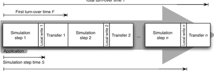
We have evaluated different application scenarios for incorporating transfer of (usually large) data files on a running Grid application. As evaluation criteria, we define the following four measurable time intervals: total turn-over time (T ) is the total (wall clock) time the application is running, including both simulation and data result transfers; first turn-over time (F ) is the (wall clock) time it takes to make the first result data available to the user (e.g., on a Grid’s SE); simulation step time (S) is the average (wall clock) time a simulation step takes to complete, until the output data is locally available on the WN to be transferred; finally, complete simulation time (C) is the average (wall clock) time the application takes from start until it finishes the last simulation step (i.e., it is T minus the average time of a data transfer step). Figures 1–4 depict these four time intervals in different application scenarios.

We have identified two main application scenarios to evaluate: serial, where data transfer and computational steps alternate, but the application is either sim-ulating or transferring, and threaded, where data transfer occurs at the same time as the next computational step, thus overlapping data transfers with computation. The serial scenario establishes a baseline of the time intervals (defined above) to which the threaded scenario is compared against. It would be expected that the threaded scenario would always yield better performance; however, results show that a serial scenario might also be the best choice in some situations.

3.1 Serial

There are two relevant variants of the serial scenario of applications:

Serial data first (DF): In this scenario, the output data is transferred as soon as it is ready, thus the application alternates between a simulation step and a transfer step (Figure 1). The transfer step can be seen as making part of the simulation, since the application must finish the transfer of the data results of one step before it can continue to the next simulation step. We expect F to be the shortest on this scenario, which might be useful for interactive Grid applications (e.g., I2G).

(5)

Application

Simulation step time S

Total simulation time C

Transfer 1 Simulation step 1 Local write 1 Simulation step 2 Local write 2 ... Simulation_step_n Local write n Transfer 2 Transfer n

Total turn-over time T

First turn-over time F

Fig. 1. Serial data first (DF) scenario variant: the application alternates between a sim-ulation step and a transfer step.

Application

Simulation step 1 Local write 1 Simulation step 2 Local write 2 ... Simulation step n Local write n Transfer 1 ... Transfer n

Fig. 2. Serial data last (DL) scenario: the application completes the simulation and only after that it initiates the transfer of the result data.

Serial data last (DL): In this case, all simulation steps are done first, and data transfers only start after that calculation phase is over (Figure 2). This vari-ant scenario is not relevvari-ant as a whole for our purpose, since it only starts transferring when the complete output is available, thus not solving one of the problems we want to address: the lack of local storage space in the WN. Besides, implementing such a scenario is very simple and can be done using a script that would transfer the whole data after the simulation is done. How-ever, we found this variant scenario useful to measure the shortest C, that is, the total time the simulation would take if a user would be running it in a desktop machine, and not on the Grid. Thus, the difference between C in this scenario and T in other scenarios is a measurement of the penalty of data transfer on the application.

3.2 Threaded

The serial scenarios described previously, although with some minimal advantages, serve mainly to establish a minimal F (scenario DF) and a minimal C (scenario DL), in order to evaluate the penalty that a threaded approach might have on those two parameters. It also establishes a T (total turn-over time) that we aim to improve.

However, the best results might be achieved if we transfer the results of a previous simulation step while the application is calculating the next simulation

(6)

step, thus overlapping data transfer and computation. This allows for optimal overlap of two tasks that have minimal influence on each other: the simulation step, which is CPU and memory intensive, but has little effect on IO, and network transfer, which stresses mainly the IO (local storage and network) and has a lesser impact on the CPU. This overlapping can be achieved by launching a transfer thread as the last step of each simulation cycle for the network transfer of the data. This data threaded scenario (DT) is the third scenario we will evaluate.

3.3 Data intensity

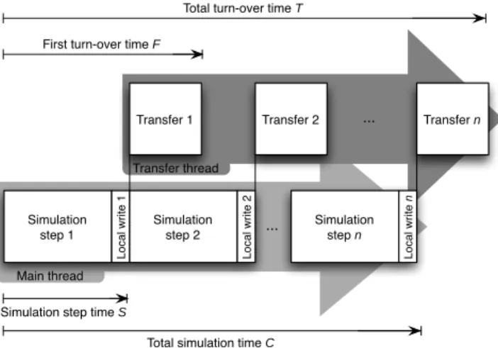
Overlapping data transfers and calculation leads to two new variants of the DT scenario, depending on the amount of data generated per simulation step: Data weak: In this scenario, the transfer time of the data result from a simulation

step is usually shorter than the duration of that step (Figure 3). This means that data transfers can occur as soon as data is available. We expect T to be much shorter than in the corresponding DF and DL scenarios, while F will not be much larger than in the DF scenario, and C will not be much larger than in the DL scenario.

Main thread Transfer thread Simulation step 1 Local write 1 Simulation step 2 Local write 2 ... Simulation step n Local write n Transfer 1 ...

Transfer 2 Transfer n

Fig. 3. Weak data threaded (W-DT) scenario: data transfers occur on a different thread than the simulation and take usually less time than one simulation step.

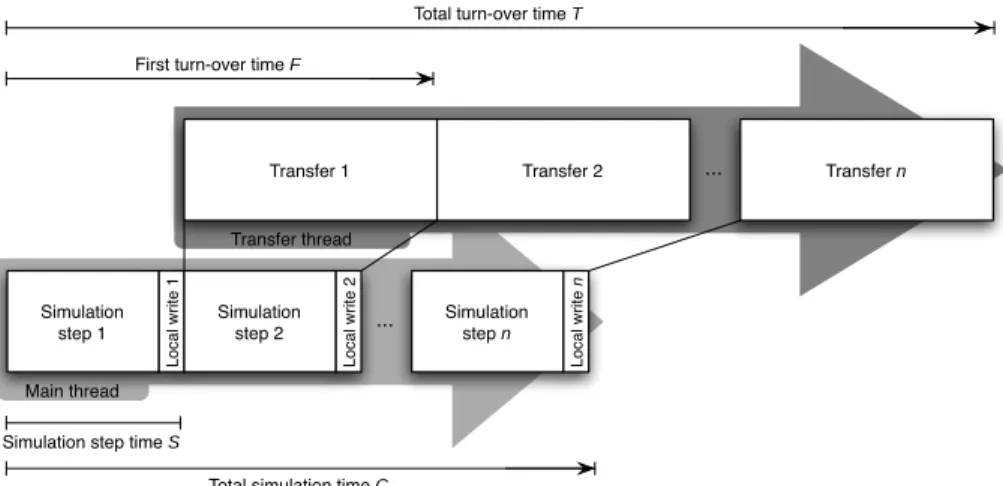
Data intensive: In this scenario, each data transfer takes longer than the aver-age simulation step (Figure 4). As a result, although time gains will still be substantial when compared to DF and DL scenarios, we expect them to be more influenced by the transfer thread.

These two threaded variants can only be compared against the corresponding serial variants, i.e., against a DF and a DL where the simulation step takes the same amount of time. Thus, we also define the corresponding variants for the serial scenarios: weak data first (W-DF), weak data last (W-DL), intensive data first (I-DF) and intensive data last (I-DL).

(7)

Main thread Transfer thread Simulation step 1 Local write 1 Simulation step 2 Local write 2 ... Simulation step n Local write n

Transfer 1 Transfer 2 ... Transfer n

Fig. 4. Intensive data threaded (I-DT) scenario: data transfers occur on a different thread than the simulation and take usually longer time than one simulation step.

3.4 Algorithm

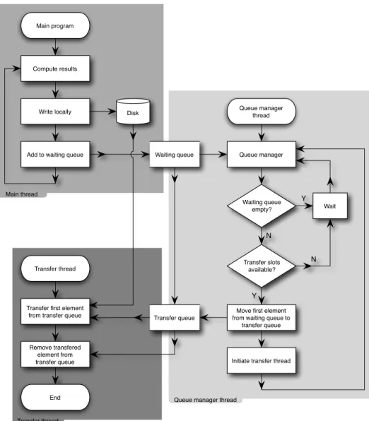
We have developed and implemented an application to test the different scenarios outlined previously. It uses an algorithm that is flexible enough to allow for multiple transfer threads to occur, for optimizing the bandwidth usage at the cost of some processing time, although that possibility is not analysed in the current paper. In Figure 5 we show a simplified fluxogram of the application.

The main loop of the application (top left of Figure 5) consists of a simulation cycle followed by a write of the result data to local storage; these two steps are repeated until the complete simulation finishes. Each local write operation is stored in a waiting queue of files waiting to be transferred.

The first time the main thread writes to this queue, it launches also a queue manager thread (right hand side of Figure 5), which is responsible for managing the waiting queue. This queue manager dispatches the files on the waiting queue list in a FIFO order to a transfer queue. It checks if there is enough transfer slots available (these are bandwidth and system dependent) and, for each file that is moved from the waiting queue to the transfer queue, it initiates a transfer thread (bottom left of Figure 5). Launching the transfer threads from a manager thread instead of the main thread allows for greater flexibility: they can be interrupted and resumed, can occur out of order, and can be more than one running at the same time.

Each transfer thread uses a simple algorithm represented on the bottom left of Figure 5. It is up to each transfer thread to remove the file reference from the transfer queue and to remove the local file as soon as the transfer finishes.

Finally, as the complete simulation finishes, the main thread sends a signal to the queue manager thread. It waits until all queues are empty and quits, thus finishing the application.

(8)

Main thread

Transfer thread

Queue manager thread Compute results

Write locally

Add to waiting queue

Disk Waiting queue Waiting queue empty? Transfer slots available? Wait

Move first element from waiting queue to

transfer queue

Initiate transfer thread Transfer queue

Transfer thread

Transfer first element from transfer queue

Remove transfered element from transfer queue End N Y Y N Queue manager Main program Queue manager thread

Fig. 5. A simplified fluxogram of the algorithm implemented to allow for simultaneous Grid simulation and network transfer of results.

4 Results and analysis

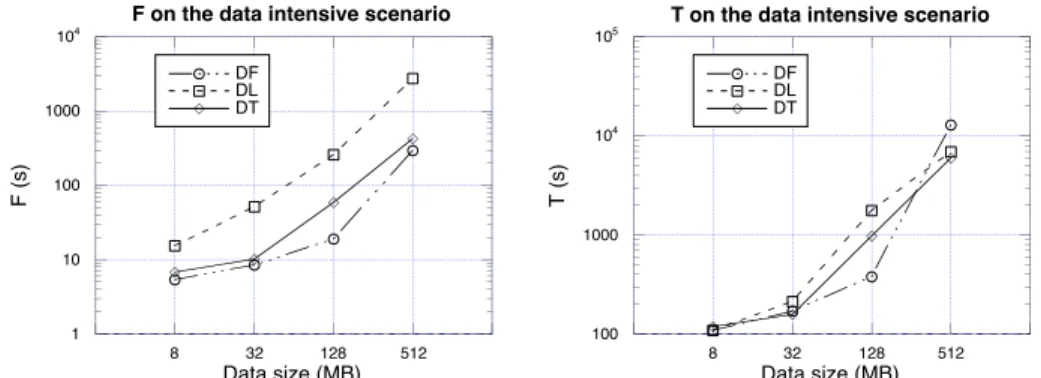
We have used the library extensively both in test and production codes. Although the library allows for multiple transfer threads, this paper focus on the use of a single transfer thread concurrently with computation. Tables 1 to 4 list the relevant time intervals obtained when using our library in a test simulation. Times are averaged over 20 runs and are measured for data sizes of 8 MB (Table 1), 32 MB (Table 2), 128 MB (Table 3), and 512 MB (Table 4). Figures 6 and 7 show the evolution of the two more relevant time intervals defined previously for the

(9)

different data sizes: T (total turn-over time) and F (first turn-over time). Figure 6 represents the data intensive variant, and Figure 7 the data weak variant.

All tests were done on WNs with a single core 2 GHz AMD Athlon 64 bit processor with 1 GB of RAM running Scientific Linux 3.0.8 and gLite 3.0 (lcg util 1.5.2). The SE belongs to the local Grid node and has a similar configuration to the WNs. The network between the WNs and the SE was a shared 100 Mbs LAN. No other jobs were running on the WNs concurrently.

Examining the results, it is interesting to note that, although the DL scenario performs poorly in almost all criteria, the other serial scenario (DF) has better performance than the threaded scenario (DT) in several situations. On the data intensive variant (Figure 6), DF and DT are comparable for small data sizes (8 and

time Data intensive simulation Data weak simulation

interval I-DF I-DL I-DT W-DF W-DL W-DT

F 5.4 15.4 7 27 477.6 33

T 108 109 119 550 571 542

S 0.51 0.52 0.9 21.9 23.6 26.8

C 103 104 113 545 566 536

All values in seconds Table 1. Average measured time intervals for 8 MB files. time Data intensive simulation Data weak simulation

F 8.5 51 10.1 43 784 55

T 170 213 158 864 1053 945

S 1.96 2.2 2.4 37.1 38.5 47.0

C 163 205 150 858 1038 937

F 19 259 59 160 3145 179

T 378 1763 972 3192 4085 3324

S 8.6 9.0 11 149 155 166

C 367 1684 924 3181 4035 3311

F 294 2760 423 618 8946 723

T 12818 6926 5957 12357 13147 8988

S 113 127 129 421 436 437

C 5710 6706 5662 12160 12928 9702

All values in seconds Table 4. Average measured time intervals for 512 MB files.

(10)

1 10 100 1000 104 8 32 128 512

F on the data intensive scenario DF DL DT F (s) Data size (MB) 100 1000 104 105 8 32 128 512

T on the data intensive scenario DF

DL DT

T (s)

Data size (MB)

Fig. 6. Comparing the I-DT scenario (solid line) with the I-DF and I-DL using the F and T time intervals.

10 100 1000 104

8 32 128 512

F on the data weak scenario DF DL DT F (s) Data size (MB) 100 1000 104 105 8 32 128 512

T on the weak data scenario DF

DL DT

T (s)

Data size (MB)

Fig. 7. Comparing the W-DI scenario (solid line) with the I-DF and I-DL, using the F and T time intervals.

32 MB, Tables 1 and 2). But with files of 128 MB, the serial scenario has better T and F than the threaded one (Table 3). This means that the first output data will be available earlier and the application will finish sooner on the DF scenario for output files of that size. We think the main reason for this unexpected behavior is the CPU overhead in launching a data transfer using lcg utils, as explained below. For large data files (512 MB, Table 4), the DT scenario shows better performance, which is to be expected. For the data weak variant (Figure 7), DF and DT have similar performance, except for large data files, where the thread variant performs better.

The other two time intervals (S and C) show a similar trend: the threaded variant allows for earlier availability of the output data files as these files get larger, although the DF scenario is usually shorter in all the tests. The S results also point to an important penalty of transferring small files in gLite: calculating F − S results at least in about 5 s. This is the minimal time it takes to transfer files from the WN to a SE using the lcg utils, since it is the difference between the average first turn-over time and the average simulation time. We obtain these ∼ 5 s both with 8 MB and with 32 MB files. Only above that the transfer time takes significantly more. During this 5 s overhead it is to be expected that the calculation thread will suffer, since during this time the CPU is also being requested by the

(11)

transfer thread. Hence it is to be expected that performance gains of the threaded scenario will be noticeably for data files that take significantly longer to transfer than the overhead of ∼ 5 s.

4.1 Application deployment

We have deployed our library on the code Osiris [5], which is a state of the art, mas-sively parallel, electromagnetic fully relativistic Particle-In-Cell (EM-PIC) code for kinetic plasma simulations. In this code, the interaction of a large number of charged plasma particles (up to ∼ 1010_{) is modeled using a particle-mesh technique}

specially suited to this problem called PIC [1]. The particles are pushed using the interpolated electric and magnetic fields at particle positions, and the full set of Maxwell’s equations are solved using a FDTD algorithm using the electrical cur-rent from particle motion. Applications include astrophysical shocks, ultra-intense laser plasma interactions, and nuclear fusion using fast ignition.

Osiris is written in Fortran 95. In its current implementation, our library presents a C interface with only two functions exposed: one to add a file to be transferred to the waiting list (see Figure 5) that takes as the only parameter the full path of that file, and another to tell the queue manager to finish all transfers and quit that takes no parameters. The user should call the first after each file is saved, and the latter at the end of the simulation. As mentioned before, currently the URL of the SE is set at the compile time of the library. To integrate our library with Osiris, thus allowing it to interface with gLite and produce large output files to the Grid, two small function wrappers were written to allow direct calling of our interface from Fortran. From the Osiris point of view it was then only required to call the function that adds a diagnostic file to the transfer queue after it is written to local storage, and to call the function to terminate the queue manager at the end of the simulation, so that Osiris would wait for the last tranfers to finish. The output files are in the HDF format, which is handled transparently by our library, as any other file format (see Section 2). The whole migration process took only a few hours; we expect linking our library with other codes/languages to present a similar difficulty.

In our simulation tests, the application ran for nearly one hour, producing more than a hundred output files of very different sizes, varying from a few kB to hundreds of MB, to a total of ∼ 5.5 GB. Performance gained from moving from a DS to DT implementation were very significant: the total turn-over time T was reduced from 3378 s to 2164 s, which resulted in an improvement of over 35%. We also expect that for longer simulations, with durations of up to ∼ 100 hours, the results will even be better. Furthermore, for such simulations, receiving the output data as soon as it is produced is an added advantage when compared to other HPC batch systems.

5 Future work

One of the main strengths of the library is its simplicity. It allows for the over-lapping of computation and data transfers with a minimal effort to the developer

(12)

of the non-Grid application. The current implementation allows for setting some parameters at compile time, like the URL of the SE (not mandatory). However, we have found useful to add an initialization interface to make available such options at run time, using command line parameters to be included in a JDL file. This will allow for finer user control of the run-time parameters of the library while keeping its simplicity.

The tests presented here were run with one transfer thread and two parallel streams per transfer (the lcg cr parameter nbstreams). This was chosen in order to limit the variable parameters during this first test phase, while at the same time optimizing bandwidth. However, we want to do more complete tests on the performance of our library with multiple transfer threads, since it was build from the beginning with this feature in mind. We expect the performance gains to increase when compared to the DF scenario until the bandwidth limit is reached.

Acknowledgements

This work was partially supported by FCT, Portugal, grants SFRH/BD/17870/ 2004 and GRID/GRI/81800/2006.

References

1. C. Birdsall, A. Langdon, Plasma Physics Via Computer Simulation, Adam Hilger, UK, (1991).

2. S. Burke, S. Campana, A. Peris, F. Donno, P. Lorenzo, R. Santinelli, A. Sciab`a, gLite 3 User Guide, https://edms.cern.ch/document/722398/.

3. I. Campos, M. Plociennik, H. Rosmanith and S. Stork, “Application Support in int.eu.grid”, Proceedings of IBERGRID: 1st Iberian Grid infrastructure conference, (2007).

4. T. Delaittre, T. Kiss, A. Goyeneche, G. Terstyanszky, S.Winter, P. Kacsuk, “GEMLCA: Running Legacy Code Applications as Grid Services”, Journal of Grid Computing, 3(1–2), pp. 75–90, (2005).

5. R. A. Fonseca, L. O. Silva, R. G. Hemker, F. S. Tsung, et al., “OSIRIS: A Three-Dimensional, Fully Relativistic Particle in Cell Code for Modeling Plasma Based Ac-celerators”, in P.M.A. Sloot et al., editors, ICCS 2002, LNCS 2331, pp. 342–351, (2002).

6. L. Gargate, R. Bingham, R. A. Fonseca, L. O. Silva et al., “dHybrid: A massively parallel code for hybrid simulations of space plasmas”, Computer Physics Communi-cations, 176, pp. 419–425, (2007).

7. Hierarchical Data Format, http://hdf.ncsa.uiuc.edu/.

8. P. Kunszt, File Transfer Service User Guide, https://edms.cern.ch/document/ 591792/.

9. M. Kupczyk et al., “Migrating Desktop Interface for Several Grid Infrastructures”, Proceeding of Parallel and Distributed Computing and Networks PDCN 2004, (2004). 10. E. Laure, S.M. Fisher, A. Frohner, C. Grandi et al., “Programming the Grid with gLite”, Computational Methods in Science and Technology, 12(1), pp. 33–45, (2006). 11. G. Sipos, P. Kacsuk, “Multi-Grid, Multi-User Workflows in the P-GRADE Portal”,