Department of Economics
The Impact of the 2008 and 2010 Financial Crises on International
Stock Markets: Contagion and Long Memory
Paulo Jorge de Brito Horta
A Thesis presented in partial fulfillment of the Requirements for the Degree of Doctor in Economics
Thesis Committee:
Doctor Nuno Miguel Pascoal Crespo, Assistant Professor, ISCTE-IUL
Doctor Paulo Manuel Marques Rodrigues, Invited Associate Professor, Nova School of Business&Economics
Doctor Isabel Maria Pereira Viegas Vieira, Assistant Professor, Universidade de Évora Doctor Paulo Manuel de Morais Francisco, Invited Assistant Professor, ISEG
Doctor Luís Filipe Farias de Sousa Martins, Assistant Professor, ISCTE-IUL Doctor Sérgio Miguel Chilra Lagoa, Assistant Professor, ISCTE-IUL
I
Resumo
Nesta tese estudamos os efeitos de contágio financeiro e de memória longa causados pelas crises financeiras de 2008 e 2010 em alguns mercados acionistas internacionais. A tese é composta por três ensaios interligados. No Ensaio 1, recorremos à teoria das cópulas para testar a existência de contágio e revelar os canais “investor induced” de transmissão da crise de 2008 aos mercados da Bélgica, França, Holanda e Portugal (grupo NYSE Euronext). Concluímos que existe contágio nestes mercados, que o canal “portfolio rebalancing” é o mecanismo mais importante de transmissão da crise, e que o fenómeno “flight to quality” está presente nos mercados. No Ensaio 2, usando novamente modelos de cópulas, avaliamos os efeitos de contágio provocados pelo mercado acionista grego nos mercados do grupo NYSE Euronext, no contexto da crise de 2010. Os resultados obtidos sugerem que durante a crise de 2010 apenas o mercado português foi objeto de contágio; além disso, conclui-se que os efeitos de contágio provocados pela crise de 2008 são claramente superiores aos efeitos provocados pela crise de 2010. No Ensaio 3, abordamos o tema da memória longa através do estudo do expoente de Hurst dos mercados acionistas da Bélgica, E.U.A., França, Grécia, Holanda, Japão, Reino Unido e Portugal. Verificamos que as propriedades de memória longa dos mercados foram afetadas pelas crises, especialmente a de 2008 – que aumentou a memória longa dos mercados e tornou-os mais persistentes. Finalmente, usando cópulas mais uma vez, verificamos que as crises provocaram, em geral, um aumento na correlação entre os expoentes de Hurst locais dos mercados foco das crises (E.U.A. e Grécia) e os expoentes de Hurst locais dos outros mercados da amostra, sugerindo que o expoente de Hurst pode ser utilizado para detetar efeitos de contágio financeiro. Em síntese, os resultados desta tese sugerem que comparativamente com períodos de acalmia, os períodos de crises financeiras tendem a provocar ineficiência nos mercados acionistas e a conduzi-los na direção da persistência e do contágio financeiro. Palavras-chave: contágio financeiro; canais de contágio; crises financeiras de 2008 e 2010; mercados acionistas; teoria das cópulas; expoente de Hurst; memória longa; eficiência.
II
Abstract
In this thesis we study the effects of financial contagion and long memory caused by the 2008 and 2010 financial crises to some international stock markets. The thesis consists of three connected essays. In Essay 1, we use copula models to test for financial contagion and to unveil investor induced channels of financial contagion to the Belgian, French, Dutch and Portuguese stock markets (NYSE Euronext group), in the context of the 2008 crisis. We find that contagion is present in these markets, the "portfolio rebalancing" channel is the most important crisis transmission mechanism, and the "flight to quality" phenomenon is also present in the markets. In Essay 2, using copula models again, we assess contagion effects of the Greek stock market to the markets of the NYSE Euronext group, in the context of the 2010 crisis. Our findings show that, during the 2010 crisis, contagion existed only in the Portuguese market, and that contagion effects of the 2008 crisis were clearly more intense than those caused by the 2010 crisis. In Essay 3, we address the subject of long memory by studying the Hurst exponents of stock markets of Belgium, France, Greece, Japan, the Netherlands, Portugal, UK and US. We find that the long memory properties of the markets were affected by the crises, especially the 2008 crisis – which moved markets towards long memory and persistence. Finally, we use copula models once more to observe that crises caused, in general, an increase in correlation between the local Hurst exponents of the markets of origin of the crises (US and Greece) and the local Hurst exponents of the other markets, suggesting that the Hurst exponent can be used in the assessment of financial contagion. In summary, the results of this thesis suggest that compared to tranquil periods, the crisis periods tend to cause inefficiency in stock markets and to lead the markets towards persistence and financial contagion.
Keywords: financial contagion; contagion channels; 2008 and 2010 financial crises; stock markets; copula models; Hurst exponent; long memory; efficiency.
III
Contents
I.Introduction ... 1
II.Main methodology ... 8
III. The Hurst exponent ... 21
IV. Essay 1 – Unveiling Investor Induced Channels of Financial Contagion in the 2008 Financial Crisis using Copulas ... 27
1. Introduction ... 29
2. Channels of financial contagion ... 32
3. Data and methodology ... 36
4. Empirical results and discussion ... 42
5. Conclusion ... 48
References ... 49
V.Essay 2 – Contagion effects in the European NYSE Euronext stock markets in the context of the 2010 sovereign debt crisis ... 53
1. Introduction ... 55
2. Financial contagion in the context of the 2010 sovereign debt crisis ... 57
3. Data and methodology ... 60
4. Results and discussion ... 66
5. Conclusion ... 73
References ... 75
VI.Essay 3 – The impact of the 2008 and 2010 financial crises on the Hurst exponents of international stock markets: implications for efficiency and contagion ... 78
1. Introduction ... 80
2. Brief literature review on the Hurst exponent and market efficiency ... 82
3. Data and methodology ... 86
4. Results and discussion ... 94
5. Conclusion ... 110
References ... 112
VII.Final remarks ... 116
IV
Tables
ESSAY 1
Table 1 – Adjusted ARMA-GARCH models to the returns under study….………42 Table 2 – Selected distribution functions for the univariate series of filtered returns…..…44 Table 3 – Selected copulas………..……….…46 Table 4 – Results of the first test: does contagion exist?....……….…47 Table 5 – Results of the second test: wealth constraints versus portfolio rebalancing....…48 Table 6 – Results of the third test: cross market rebalancing versus flight to quality.….…48
ESSAY 2
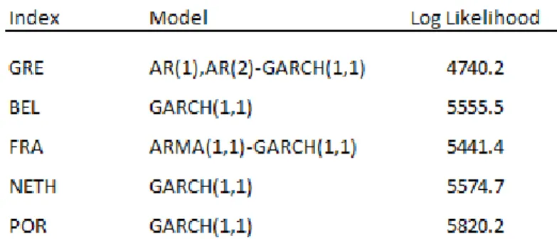
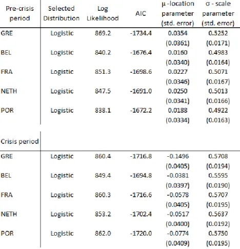
Table 1 – Estimated models for the series of indices..……….………66 Table 2 – Distribution functions for the series of the filtered returns……….……….……68 Table 3 – Selected copulas models………..….………69 Table 4 – Tests of financial contagion……….………71 Table 5 – Tests of intensity difference of Subprime and European debt crises…….…..…72 Table 6 – Sensitivity analysis to the dating of the sovereign debt crisis…….……….……73 ESSAY 3
Table 1 – Hurst exponents obtained using the MFDMA technique, for eight finite samples of white Gaussian noises………..……….………94 Table 2 – Results of Test 1: presence or absence of long memory...……….……96 Table 3 – Selected copula models for the local Hurst exponents...………..…………..…105 Table 4 – Results of Test 2: increase in correlation between local Hurst exponents...…107 Table 5 – Public finance situation in 2010 (source: OECD Economic Outlook)…...…109
V
Figures
Figure 1 – Example of distribution functions obtained from Clayton and Gumbel copulas ...12 Figure 2 – Draft of the R interval of a reservoir (source: Rêgo, 2012) ……….………..…25 ESSAY 1
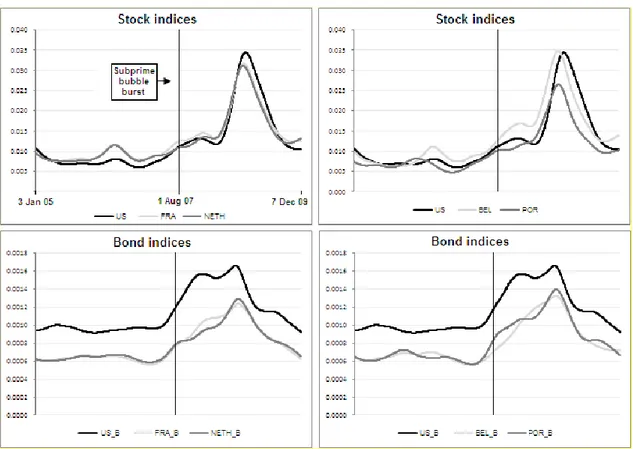
Figure 1 – Investor induced channels of transmission of the Subprime financial crisis..…34 Figure 2 – Volatility trends of filtered stock and bond returns………....…43
ESSAY 2
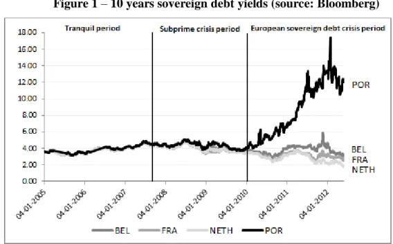
Figure 1 – 10 years sovereign debt yields (source: Bloomberg)………….……….60 Figure 2 – The trend of the conditional volatility of filtered returns…..……….67
ESSAY 3
Figure 1 – Estimates of Hurst exponents for eight stock markets in four different
periods………...98 Figure 2 – Local Hurst exponents and raw stock indices for the tranquil period, the
1
I. Introduction
In this thesis we study the effects of financial contagion and long memory caused by the 2008 and 2010 financial crises to some international stock markets. We use copula models as the main framework for the assessment of financial contagion, and we use the Hurst exponent calculated with the multifractal detrended moving average technique (MFDMA) for the evaluation of long memory.
In the following paragraphs we provide a brief overview of the importance of studying financial contagion and long memory. We first start with financial contagion. Financial contagion
The 2008 financial crisis started in mid-2007 with the turbulence in the Subprime segment of the United States (US) housing market, which spilled over to the global financial system.
To avoid a catastrophic collapse of the financial markets and real economy, the general response to the crisis consisted of three main interventions by governments across the globe: 1) bailouts and injections of money into the financial system to keep credit flowing; 2) cutting interest rates to stimulate borrowing and investment; and 3) extra fiscal spending to shore up aggregate demand (Islam and Verick, 2010).
Despite the efforts, the authorities could not contain the spill over of the financial crisis to the real economy. In December 2007 the US fell into a recession and the financial crisis rapidly mutated to the worst recession the world has witnessed for over the last six decades. Important economies in the European Union (EU) and Japan went collectively into recession by mid-2008 (Islam and Verick, 2010).
One consequence of the extra fiscal spending was the rapid increase of government debts, and some European countries, such as Greece, with high levels of sovereign debt, experienced a decrease of confidence by international investors, which led to the 2010 European sovereign debt crisis, started in Greece in late 2009.
The 2008 financial crisis brought severe discredit on regulatory authorities, both national and global, responsible for foreseeing, controlling and managing financial changes.
2 In response to the severe disruption of the system, the agenda defined by the Group of Twenty (G20) in 2008 has led to reforms aimed at providing a new regulatory framework in order to improve financial stability (Perrut, 2012).
Most of the regulatory measures were taken bearing in mind the soundness of the banking system and the prevention of systemic risk. For example, the Financial Stability Board (FSB) and the Basel Committee on Banking Supervision (BCBS) created a new tool with a macro-prudential goal in the new banking framework, the so called Basel III standard. The FSB also expanded the concept of Systemically Important Financial Institutions (SIFI). Now, it is not just the size of the institution that matters in evaluating SIFI, but also matters the liquidity situation of the institutions and the off-balance sheet relations between banks, especially through credit insurance mechanisms, such as credit default swaps (CDS) (Perrut, 2012).
At the level of securities markets, the International Organization of Securities Commissions (IOSCO) has also identified reducing systemic risk as one of the key objectives of securities regulation. One key element of systemic risk in securities markets is the channel through which the negative consequences of a triggering event is transmitted between markets. In this respect, IOSCO (2011) identifies correlation between assets as a mean through which systemic risk may propagate.
According to IOSCO (2011), correlation is the tendency of the prices of different assets to move together or be similarly affected by an event or the release of new information. Correlated assets can transmit risk from one part of the system to another through changes in asset prices. When investors have similar portfolio holdings or employ similar strategies, sharp changes in the price of a particular asset can lead multiple market participants to make similar portfolio decisions. Individually, these decisions by themselves would not pose a systemic risk. However, when considered collectively, these potentially rational decisions can have a significant impact on asset prices and market liquidity. Under these circumstances, the assets prices can fall sharply and the liquidity can evaporate rapidly, because an increase in uncertainty regarding market conditions can quickly lead to the withdrawal of participants from a market. Large price declines could cause a further
3 deterioration of available liquidity as participants may be less willing to transact in a falling market.
Also, reduced liquidity can result in fire-sale type scenarios for those forced to exit a position in an illiquid market. It can also cause firms to have to sell other assets in other markets. This can then cause the illiquidity in one market to impact asset values in another (IOSCO, 2011).
In such scenarios, possible cases of market abuse may also arise.
The correlation between different assets prices and its potentially amplifying effect can lead to systemic risk concerns if it is not fully understood by market participants or if it changes over time. Changes in correlation can be dramatic during times of financial stress. When correlations change, market participants become less able to predict how the price of one asset may respond to other changes (IOSCO, 2011).
In this thesis we intend to improve the understanding of correlation and its changes over time during the recent financial crises, with the purpose of providing information to market participants, including securities regulators and portfolio managers. The study of correlation leads us to the definition of financial contagion of Forbes and Rigobon (2002). According to these authors, contagion (shift-contagion) exists when we face "a significant increase in cross-market linkages after a shock to an individual country (or group of countries)." From a practical standpoint, it is considered that the stock markets are facing contagion when the correlation between returns of market indices experiences a statistically significant increase from a period of stability to a period of financial distress. This is the definition of financial contagion adopted in this thesis1.
1
Although we use the definition of contagion of Forbes and Rigobon (2002), there are other definitions adopted in the literature. See Forbes and Rigobon (2002), Pericoli and Sbracia (2003) or Constâncio (2012) for some examples of different definitions.
According to Forbes and Rigobon (2002), the definition presents two operational advantages, which are relevant for the empirical analysis developed in this thesis. Horta et al. (2010) also emphasize these advantages: first, the definition provides a straightforward framework to test for the existence of contagion, simply by checking whether there are significant increases in cross market linkages after a crisis; second, it avoids to distinguishing between mechanisms of crisis transmission.
It is worth noting the difference between interdependence and contagion in stock markets. While interdependence usually refers to a significant correlation between stock market returns, contagion refers to a significant increase in such
4 Considering the above mentioned relation between correlation and systemic risk, it is worth mentioning that a way of containing the propagation of such risk is to mitigate or prevent the signs of financial contagion that arise in stock markets. The framework we present in this thesis is useful in this respect, since it provides a way to assess financial contagion between stock markets. If securities regulators implemented our framework, maybe they would be capable to early detect potential situation of financial contagion and take timely measures to prevent the excessive propagation of risk between markets.
Several measures can be taken by securities regulators to avoid the potential increasing in correlation between stock markets during financial distress periods, and thus mitigating financial contagion.
For example, at the height of the financial crisis in September 2008, competent authorities in several EU Member States and supervisory authorities in third countries, such as the US and Japan, adopted emergency measures to restrict or ban short selling in some or all securities. They acted due to concerns that at a time of considerable financial instability, short selling could aggravate the downward spiral in the stock prices, notably in stocks of financial institutions, in a way which could ultimately threaten their viability and create systemic risks (Regulation, 2012).
Moreover, the recent European Union regulation No 236/2012 on short selling and certain aspects of credit default swaps (Regulation, 2012) grants powers of intervention to require further transparency or to impose temporary restrictions on short selling, CDS and other transactions in order to prevent a disorderly decline in the price of financial instruments.
The EU Directive 2004/39/EC of the European Parliament and of the Council, of 21 April 2004, on markets in financial instruments (MIFID, 2004), in its article 50/2/j, provides relevant tools to contain contagion, since it grants powers to securities regulators to require the suspension of trading in a financial instrument whenever trading is expected to undermine the price formation process or prejudice the investors inter alia. Suspending financial instruments from trading forces correlation between assets to decrease because the market price of the suspended asset remains unchanged, while the price of other assets varies freely, according to the market forces of demand and supply.
5 Long memory
The concept of long memory (or long-range dependence) means that there still is high correlation between events that are remote in time. For a series of daily returns, this means that the return of period t is correlated with a distant return, in period 100 or t-1000, for instance. Long ago, the British hydrologist Edwin Hurst found that the floods of Nile River exhibit long memory and he constructed a simple parameter (called H or Hurst exponent) to summarize the phenomenon of long memory.
Long memory can be positive or negative. It is positive when there is a higher than 50% probability that a positive (negative) data point of a series is preceded by a positive (negative) data point of the same series. And it is negative when there is a higher than 50% probability that a positive (negative) data point is preceded by a negative (positive) data point (Rêgo, 2012).
These characteristics of long memory are captured by the parameter H. Thus, values of H ranging from 1/2 to 1 are indicative of positive long memory, and values of H ranging from 0 to 1/2 are indicative of negative long memory. H=1/2 indicates absence of long memory and is consistent with the efficient market hypothesis (Da Silva et al., 2007).
The study of long memory in stock markets is of interest because, for example, the knowledge of the long memory characteristics of a series provides information on the efficiency of markets. Fama (1970) states that a market in which prices always fully reflect available information is called efficient. For investors this is relevant because if a market is inefficient (i.e. if the market exhibits long memory) then there is an opportunity to obtain abnormal returns in this market. For example, if pt represents a stock price in a moment t, and if an investor knows that the stock price exhibits positive long memory, then if the asset price rises in two consecutive trading sessions, pt1 pt, the investor anticipates that
it is more likely the next movement of the price is an upward movement,
pt2 pt1
P pt2 pt1
P . In such conditions, if the investor buys the stock in moment
t+1, then it is more likely to obtain a profit in t+2 than to suffer a loss2.
2 Long-memory is a long-term phenomenon. Therefore, events that influenced the values of a series long time ago also influence the values of a series in the short-term.
6 In this thesis we study the behavior of the exponent H over time to shed light how the 2008 and 2010 financial crises influenced the long memory and the efficiency characteristics of the markets in the sample. We also relate long memory with our findings in financial contagion to the extent that we observe a significant increase in correlation between some local Hurst exponents, from tranquil to crisis periods.
The Essays
The thesis consists of three connected essays. In summary, the main topics and contributions of the essays are the following. In Essay 1, we use copula models to test for the existence of financial contagion and to test investor induced channels of financial contagion to the Belgian, French, Dutch and Portuguese stock markets (markets of the NYSE Euronext Group), in the context of the 2008 financial crisis. Until now, copula models have been used in the literature to measure financial contagion. As a novelty, we propose to extend the scope of such models, suggesting their use in unveiling the channels through which crises propagate. We also provide information on stock markets co-movements, useful to improve portfolio management. The main research questions of Essay 1 can be summarized as follows: i) Is there financial contagion in the stock markets of the sample, in the context of the 2008 financial crisis? ii) Which channel was most active in the propagation of the 2008 crisis: the wealth constraint channel or the portfolio rebalancing channel? iii) Which sub-channel was most significant in the propagation of the 2008 crisis: the cross-country portfolio re-balancing sub-channel or the domestic flying-to-quality phenomenon? In Essay 2, we analyze the contagion effects of the Greek stock market to the European stock markets of Belgium, France, the Netherlands and Portugal, in the context of the 2010 European sovereign debt crisis. We perform two tests of contagion and provide a methodology based on copula models and bootstrap procedures to compare contagion intensities between different crises. The first test assesses the existence of contagion on the relevant markets and the second compares contagion intensity during the 2008 financial crisis and the 2010 European sovereign debt crisis. The main research questions of Essay 2 can be summarized as follows: i) Is there financial contagion in the stock markets of the sample, in the context of the 2010 financial crisis? ii) Which crisis affected more significantly the stock markets of the sample: the 2008 or the 2010 financial crisis? In Essay 3, we evaluate the impact that the 2008 and 2010 financial crises caused to
7 the dynamics of the Hurst exponents of indices representing the stock markets of Belgium, France, Greece, Japan, the Netherlands, Portugal, UK and US. We propose the use of copula models to evaluate the dependence structure between local Hurst exponents of different pairs of indices returns and we also propose a new application for the Hurst exponent: the assessment of financial contagion between stock markets. This means that instead of using market returns to observe a significant increase in correlations from a tranquil to a crisis period, we use local Hurst exponents to obtain the same significant increase in correlations. The main research questions of Essay 3 can be summarized as follows: i) Do the 2008 and 2010 financial crises affected the long memory properties of the stock markets of the sample? ii) Do the 2008 and 2010 financial crises caused an increase in the correlation between the returns’ local Hurst exponents for the markets where the crises originated (US and Greece, respectively) and those of the other markets in the sample?
Thesis overview
The thesis is organized as follows. In chapter II we explain the mathematical concept of copula, since copulas are the basic framework we use in the three essays. Basically, a copula is a joint distribution function of random variables, with the specificity that the marginal random variables follow uniform distribution functions in the interval [0,1]. Copula models were introduced in finance literature in 1999 (Aas, 2004) and are useful to evaluate the dependence structure between returns. In chapter III, we provide a brief description of the origin of the Hurst exponent and we relate the exponent to the concept of long memory, which we use in Essay 3. Then, in chapters IV, V and VI we present the three essays. The first essay is entitled “Unveiling investor induced channels of financial contagion in the 2008 financial crisis using copulas”; the second is entitled “Contagion effects in the European NYSE Euronext stock markets in the context of the 2010 sovereign debt crisis”; and the third is entitled “The impact of the 2008 and 2010 financial crises on the Hurst exponents of international stock markets: implications for efficiency and contagion”. Finally, in chapter VII we draw the main conclusions of this thesis.
8
II. Main methodology
II.1. Mathematical concept of copula
The concept of copula was introduced by Sklar (1959). A copula is a multivariate distribution with uniform marginal distributions in the interval [0,1].3
Sklar (1959) showed that it is possible to separate a joint distribution function in its two basic components: the marginal distribution functions of the variables and the dependence function between the marginal variables (i.e., the copula).
An important tool to Sklar's theorem is the fundamental result of the theory of random number generation, demonstrated by Fisher (1932), which states that if X is a continuous random variable with distribution function F, then U F
X follows a uniform distribution between 0 and 1, regardless the form of F. The variable U is known in the literature as the “probability integral transform” of X (vd. Patton, 2002). In other words, a copula is a function that allows one to connect the univariate distribution functions to the joint distribution function. It was due to this feature of connection that Sklar attributed the name "copula" - a Latin word which means "link" or "bond" (Patton, 2002).Formally, the Sklar's theorem states that any d-dimensional distribution functionF, with univariate marginal distribution functions F ,...,1 Fd, can be written as follows:
x xd
C
F
x Fd
xd
F 1,..., 1 1 ,..., , (1)
where C is the copula.
Alternatively, if X
X1,...,Xd
is a vector of random variables, then the copulafunction is given by:
3In this thesis we only use continuous bivariate copulas. These copulas have domain in the unit square and codomain in the unit interval:
0,1 0,1 0,1.9
u ud
F
F
u Fd
ud
C 1,..., 11 1 ,..., 1
(2)
where Fi1 is the inverse of the marginal distribution function Fi , and Ui ~ Unif
0,1 , di1,..., (see the proof in Nelsen, 2006).
If we derive both sides of Equation 1 with respect to each of the marginal variables, we obtain the probability density functions (in lowercase), and the dependence structure role of the copula becomes clearer:
d d d d d d d d d d d x x F x x F x F x F x F x F C x x x x F ... ... ,..., ... ,..., 1 1 1 1 1 1 1 1 1 (3) or
x xd
c u ud
f
x fd
xd f 1,..., 1,..., 1 1 ... (4)Equation 4 shows that if the density function of the copula is neutral,
u1,...,ud
1c , then the joint density function is equal to the product of the marginal density functions, meaning in this case that all the variables in the vector X
X1,...,Xd
are independent. Conversely, if the density function of the copula is not neutral, then it necessarily represents the dependence structure between the variables in vector X .
Another important aspect of the Sklar’s theorem is that it allows a good flexibility in multidimensional modeling. For example, knowing the marginal distribution functions (which need not to be identical) and knowing the copula function (which can be chosen independently of the marginal distributions), then the joint distribution function can be directly obtained by applying the theorem.
In this thesis, as one of our objectives is the modeling of the dependence structure of pairs of financial time series, then selecting the appropriate distribution functions for the univariate variables, and choosing an adequate copula model to connect these variables, we
10 are able to analyze the dependence structure and the co-movement between the series, using the data points resulting from the probability integral transform of the marginal variables as input to estimate the copula (Equation 2).
This means that we can easily avoid Gaussian models which, as the literature has shown, have some limitations in financial time series, given the features which characterize some of these series, such as heavy tails or stochastic volatility (ARCH effects). Also in terms of bivariate modeling, several studies have shown that the bivariate Gaussian distribution may not be the most appropriate model in some situations because it does not captures the asymmetric dependence which often exists in two-dimensional series. For example, if two assets returns are more correlated in periods of downward markets than in periods of upward markets, then the Gaussian distribution does not capture these situations because the "lower tail" of the true distribution is tighter (i.e., exhibits more correlation lato
sensu) than the “upper tail”, which is more disperse. Further in this thesis, in Essay 2, we
explain the advantage of using copulas for analyses of financial contagion, rather than other common methodologies, such as the Pearson’s linear correlation coefficient.
There is an extensive variety of copulas proposed in the literature (vd. Nelsen, 2006), but the most widely used in finance are usually the Gaussian copula, proposed by Lee (1983), the Student-t copula and some copulas of the Archimedean family, such as the Gumbel (1960), Clayton (1978) or Frank (1979) copulas. These copulas have shown to adjust reasonably to financial time series.
If the variables under study present a symmetric dependence structure, then Gaussian or Student-t copulas may be appropriate for their modeling. If the dependence is stronger in the left tail of the distribution, the Clayton copula can be a good choice, as the Gumbel copula may be a good choice for variables with dependence on the right tail (Trivedi and Zimmer, 2005). Note that these two latter copulas do not allow modeling negative dependence structures between variables, but this is not a problem for modeling the returns of stock indices, since dependence on these cases is usually positive.
The Frank copula is symmetric but has some advantages relative to the Gaussian or Student-t copulas, namely it allows a simpler estimation of the dependence parameter, since its analytical expression is simple (explicit). The Frank copula is still appropriate in
11 modeling variables with weak dependence structures in the tails (Trivedi and Zimmer, 2005).
As an example, we present the functional forms of the Clayton and Gumbel copulas4:
1 2 1 2 1, 1 u u u u CClayton (5)where
0,
is the dependence parameter between the marginal variables
1 1 1 1 F U X and
2 1 2 2 F UX , and F and 1 F are the distribution functions of 2 X and 1
2
X , respectively. As approaches zero, the variables become less dependent. Therefore, when increases the degree of dependence between X and 1 X also increases. 2
The Gumbel copula is given by the following expression:
1 2 1 2 1,u exp lnu lnu u CGumbel (6)where the dependence parameter
1,
. If 1 the variables X and 1 X are 2independent5. When increases, the dependence between the variables also increases. Figure 1 simulates Clayton and Gumbel copulas for different dependence parameters. We assume the marginal distribution functions follow standardized Gaussian models.
4 The functional forms of the copulas we used in this thesis can be obtained in Schmidt (2006), Trivedi and
Zimmer (2005) and Dias (2004).
5 The independent copula is given by
2 1 2 1,u uu u CIndep .
12 Figure 1 – Example of distribution functions obtained from Clayton and Gumbel
copulas
Figure 1 shows a random draw of 2000 data points from distribution functions obtained from: (1) Clayton copula with = 1.5; (2) Clayton copula with = 3; (3) Gumbel copula with = 2; (4) Gumbel copula with= 3. We assume that the marginal variables
1
X (horizontal axis) and X (vertical axis) follow standard Gaussian distributions. 2
Note that the data points of the distribution in panel (2), obtained from the Clayton copula, are more concentrated than the points of the distribution in panel (1), i.e. displays a higher degree of dependence. Moreover, the left side of each distribution based on the Clayton copula is tighter than the right side - where data points are dispersed.
If the distribution in panel (1) represents the dependence structure between two stock markets in a tranquil period and the distribution in panel (2) represents the dependence structure of the same markets in a crisis period, then we would probably conclude for the existence of financial contagion.
13 Besides “pure” copulas, it is also common the usage of “mix” copulas (see for example Dias, 2004). A mixture of a Gumbel and a Clayton copula, for example, captures situations of almost perfect symmetry and situations of different forms of asymmetry.
The functional form of this mix copula is the following:
u1,u2
w1C
u1,u2
w2C
u1,u2
Cmix Clayton Gumbel (7)
where w1,w2
0,1 and w1w2 1.As the weight parameter w tends to 1, the mix copula in Equation 7 tends to the 1 Clayton copula and therefore the dependence in the left side of the mix copula becomes stronger than the dependence in the right side. Conversely, when w tends to 0, it is the 1 right side of the mix copula that exhibits more dependence. It is also possible for the mix copula to capture situations of independence between variables. This happens when the dependence parameter ( ) of the Clayton copula tends to zero and the parameter of the Gumbel copula is equal to 1, simultaneously.
In addition to characterizing the dependence structure of the series, copulas also allow expressing that structure in scalar synthetic measures, such as the rank correlation Kendall’s tau ( ) or Spearman’s rho () (Schmidt, 2006). Rank correlations are also useful measures to compare the dependence structures between different copulas. Note that although each copula has its own dependence parameter ( ), that parameter is not readily comparable to the dependence parameter of other copula. For example, the variation interval of the dependence parameter of a Clayton copula is not the same as that of a Gumbel copula. While for the Clayton copula varies in the interval
0,
, in the case of a Gumbel copula varies in the interval
1,
. By contrast, rank correlations always vary between -1 and 1, and in addition are invariant to non-linear monotonous transformations of the variables, which is consistent with the use of copulas when we perform the probability integral transform of the marginal variables.14 In this thesis we use the Kendall’s tau as a synthetic measure of global dependence between financial time series6. This measure can be obtained directly from each copula
model, using the following expression (Nelsen, 2006):
1 0 2 1 1 0 2 2 1 1 2 1 2 1 , , 4 1 , dudu u u u C u u u C X X Kendall (8)In addition to rank correlation measures, it is common to use the asymptotic tail coefficients extracted from copulas (U and L) to measure the (local) dependence between variables in the tails of the bivariate distributions. These coefficients measure the probability that a random variable reaches an extreme value knowing that another random variable has also reached an extreme value. For example, to measure the probability of a stock return experience a large decrease knowing that another stock return has already faced a large decrease, we use the asymptotic lower tail coefficient (L), which is defined formally as follows (see for example Schmidt, 2006):
)) ( ) ( ( lim 2 21 1 1 1 0P X F q X F q q L (9)
Similarly, the asymptotic upper tail coefficient is defined by:
)) ( ) ( ( lim 2 21 1 11 1P X F q X F q q U (10)
Next, we present the functional forms of the copulas used in this thesis, with their correspondent tail coefficients and Kendall’s tau parameters (vd. Trivedi and Zimmer, 2005; Schmidt, 2006; Grossmass, 2007).
6 Using the Kendall’s tau and the Spearman’s rho statistics, Horta et al. (2010b) performed a test of financial
contagion for a set of seven developed stock markets, in the context of the Subprime crisis. The results obtained based on the Kendall’s tau were virtually identical to those obtained using the Spearman’s rho, thus confirming that these two statistics are close substitutes.
15 Frank Copula , (11) , , , . Clayton Copula (12) Gumbel Copula , where , (13)
16
Gaussian Copula
(14)
where denotes the cumulative distribution function (cdf) of a standard normal distribution and is the cdf for a bivariate normal distribution with zero mean and covariance matrix , a matrix with 1 on the diagonal and otherwise (see Schmidt, 2006).
t Copula
(15)
where denotes the Student-t distribution function with degrees of freedom.
17 , . Clayton-Gumbel Copula (16) , where and
Gumbel-Survival Gumbel Copula
(17)
where and , and the survival copula is given by:
18
Clayton-Gumbel-Frank Copula
(18)
where and
II.2. Fitting the copula parameters: the IFM method
The IFM method means "inference functions for margins" (McLeish and Small, 1988) and consists of estimating the model parameters by finding the roots of a set of inference functions. In the case of the maximum likelihood estimation, the inference functions are the partial derivatives of the logarithm of the likelihood function, i.e. the score functions (Dias, 2004). Next we briefly describe the method following Dias (2004).
Consider the vector X
X1,X2
t of random variables. Our aim is to estimate the parameters of the following model for X , obtained from the Sklar’s theorem:
x1,x2;1,2,
C
F1
x1;1
,F2 x2;2
;
F
(19)
where Fi
xi;i
is the distribution function of Xi with vector parameters i, i =1,2, andC is the copula with parameter . The latter parameter is a scalar, since we are only considering two marginal variables.
If we take first derivatives to both sides of Equation 19 with respect to each of the marginal variables, we obtain the probability density functions - represented in lowercase:
19
2
2 2 2 1 1 1 1 2 2 2 1 1 1 2 2 2 1 1 1 2 2 1 2 1 2 1 2 ; ; ; ; , ; , ; , , ; , x x F x x F x F x F x F x F C x x x x F (20) or
2 1 2 2 2 1 1 1 2 1 2 1, ; , , ; , ; ; ; i i i i x f x F x F c x x f (21)Using logarithms we obtain:
2 1 2 2 2 1 1 1 2 1 2 1, ; , , log ; , ; ; log ; log i i i i x f x F x F c x x f (22)Assuming we have n independent and identically distributed (iid) observations7 of a two-dimensional vector (our sample),
x1,x2
1,...x1,x2
nthen the logarithm of the likelihood function becomes:
n j i i ij i n j j j n j j j x f x F x F c x x f x L 1 2 1 1 2 2 2 1 1 1 1 2 1 2 1 2 1 ; log ; ; , ; log , , ; , log ; , , (23)The logarithm of the likelihood function for each marginal variable is given by:
;
log
, i 1,2 1 ;
n j i ij i i i x f x L (24)7 Further in this thesis, in the essays, we filter the raw returns using ARMA-GARCH models to obtain iid
20 We obtain a maximum likelihood estimate (
i
) for the parameters of the density functions of the marginal variables, solving the following equations with respect to i:
1,2 i , 0 ; ,..., 0 ; 1 i ip i i i i i x L x L (25)where pi is the number of elements in vector i, i.e. the number of parameters of the distribution function of the random variableXi. For example, if Xi follows a Gaussian distribution, the parameters are two: the mean and the variance. If Xi follows a Student-t,
the number of parameters is three: the mean, the variance and the degrees of freedom. After estimating the parameters
i
, these are placed in Equation 23, yielding the following expression:
n j i i ij i n j j j n j j j x f x F x F c x x f x L 1 2 1 1 2 2 2 1 1 1 1 2 1 2 1 2 1 , log ; , , , log ; , , , log , , ; (26)For the estimation of the copula dependence parameter,
, we maximize the log-likelihood function (Equation 26) with respect to . In other words, we solve:
0 , , ; 1 2 x L (27)
21 which is equivalent to maximizing the first parcel of Equation 26 with respect to . The second parcel is constant and does not depend on . That is,
0 ; , , , log ; 1 2 2 2 1 1 1
n j j j F x x F c x L (28) 0 ; , log 1 2 ^ 1 ^
n j j j u u c , (29) since
,
i1,2 i i i i F x u .In summary, the IFM method consists of two steps. In the first, we estimate the parameters of the distribution functions of the marginal variables, and in the second step we introduce these latter estimates in the copula function to obtain an estimate of the dependence parameter of the copula8.
III. The Hurst exponent
This chapter provides a brief description of the origin of the Hurst exponent and relates the exponent to the concept of long-term memory, which we use further in chapter VI of this thesis. For a more detailed description of the concepts discussed here, the reader could refer to Mandelbrot and Hudson (2004) and Rêgo (2012). We follow these authors.
8 Further in the thesis, in the essays, we fit different marginal and copula models to the data, and then we use
22 The Hurst exponent has been applied to different topics in the financial literature. In chapter VI we provide some examples of such applications.
The Hurst exponent ( ) is a coefficient ranging between 0 and 1 and measures the long (term) memory properties of the series. An exponent of gives an indication of a Brownian motion9 (the continuous analog to the random walk), a random process without long memory where the increments are independent and identically normally distributed, and therefore not predictable. Series presenting Hurst exponents different from 1/2 exhibit long-term memory and therefore their increments are not independent, making the series predictable. Values of ranging from 1/2 to 1 are indicative of a persistent, trend-reinforcing series (positive long range dependence). In this case, there is a higher than 50% probability that a positive (negative) value of a series is preceded by a positive (negative) value of the same series. Values ranging from 0 to 1/2 suggest anti-persistence, and therefore past trends of a series tend to reverse in the future (negative long range dependence). In this case, there is a higher than 50% probability that a positive (negative) value of a series is preceded by a negative (positive) value (Da Silva et al., 2007).
The use of to represent the Hurst exponent was suggested by Mandelbrot, in honor of the English hydrologist Harold Edwin Hurst and the mathematician Ludwig Otto Hölder.
It all begins in 1906, after Hurst arrived at Cairo, Egypt, and faced a problem related to the floods of the Nile River. The annual variation of the Nile water levels was a problem misunderstood by the hydrologists at that time. Discharges of the Nile varied widely, from 151,000 million cubic meters in the rainy year of 1878-1879, up to 42,000 million cubic meters during the drought of 1913-1914. Moreover, statistical data showed that dry years were followed by other dry years, such as rainy years also tended to be followed by another rainy years. The data showed a certain time dependence on this fact of nature.
9 If follows a stochastic process known as Brownian motion or Wiener process, the increments of ,
follow a normal distribution with zero mean and standard deviation , where is the time increment corresponding to . Formally: .
23 The most obvious solution to control the flow of the river was to build a barrier that was sufficiently high to contain the water in rainy years and release the water in dry years. The challenge posed to Hurst was to determine the optimum height of the reservoir.
At that time, the engineers determined the height of the water reservoirs assuming that the annual variations of floods behaved independently, according to a Brownian motion. They assumed that the difference between the highest flood in a certain year and the lowest flood in another year depended on the square root of the number of years between the two floods. For example, assuming that in a 36-year period the highest flood is 151,000 million cubic meters, and the lowest flood is 42,000 million cubic meters, then the
difference between the two floods is . Now, if we consider,
for example, a period four times longer ( years), the formula used by the engineers indicated that the expected difference between the highest and the lowest flood
would be times higher, i.e. million cubic meters.
Thus, if someone intended to replace a 36 years old reservoir with a new one, to protect against 144 years of floods, the new reservoir should be twice higher than the former, according to the calculations of the engineers.
However, Hurst found that the difference (which he called range R) between the highest and the lowest flood grew faster than was predicted by the Brownian motion formula. For this reason, the new reservoir should have a height greater than twice the height of the old reservoir. The formula assuming a Brownian motion does not work in these cases because it ignores the exact sequence when floods occur. Instead, the Brownian motion only considers the annual volume of floods. For example, some consecutive rainy years could fill the reservoir, followed by a few years of moderate rain, but the reservoir remains full due to the effect of previous rainy years. Next, some years are dry, and the reservoir begins to empty, but it still contains more water than usual because the previous rainy years continue to have an effect. This is the source of long-term memory: the amount of rain that falls in a year has an effect on the amount of water in the reservoir not only in the same year, but also in subsequent years, and this effect extends in time, in the long term, in the limit to infinity, if there was a reservoir that lasted so long!
24 Next, we consider in more detail the analysis developed by Hurst to improve the Brownian motion estimates in determining the volume of a reservoir. The analysis is known as Rescaled Range Analysis (or R/ S Analysis). We follow Mandelbrot and Hudson (2004) and Rêgo (2012) to explain the Hurst technique.
Suppose the reservoir receives an annual influx of water (t), and displays a mean annual discharge of:
1 ) ( 1 ) ( t t t . (30)If we consider that the cumulative deviation between the water influx and its mean is given by
t u t u t X 1 ) ( ) ( ) , ( , where 1t , (31)then the maximum and minimum value of X(t,) represents the maximum and minimum volume that the reservoir can take in period , without overflowing or drying. Thus, the interval R() measures the volume of the reservoir:
) , ( min ) , ( max ) ( 1 X t 1 X t R t t (32)
For example, when consecutive floods occur more often (i.e., when more time dependency exists in a series), the maximum of X(t,) is higher and, therefore, the value of R() becomes larger, implying more intense (positive) long memory in the series.
25 Figure 2 – Draft of the R interval of a reservoir (source: Rêgo, 2012)
Besides the flooding of the Nile River, Hurst investigated other natural phenomena and found the presence of long memory in many of such phenomena.
To compare the intervals of various different phenomena, Hurst used the ratio, where represents the standard deviation of (t) obtained by the following equation, as usual:
12 1 2 ) ( ) ( 1
t t t S (33)Hurst found empirically that when the sample size ( ) varies, the ratio followed a power law relationship described by:
(34) where represents the Hurst exponent.
A power law relationship means that when we consider various values for , and
when we obtain the logarithms for both sides of Equation 34, , the
relationship between and becomes linear, and the slope can be obtained, for example, through an ordinary least squares regression.
26 The existence of such power law (or scaling) is a sign of fractality of a series. Synthetically, a series exhibits fractality when a part of the series behaves identically or similarly to the whole series. In other words, even if one considers various parts of the original series (corresponding to various ), the remains unchanged, the scaling relation or power law remains the same10.
Hurst found that most phenomena he analyzed, behaved similarly to the case of Nile River. This means that when he graphed the number of years and the interval between the largest and smallest record ( ), he reached the conclusion that this interval increased too fast, just as in the case of Nile River. The phenomena examined by Hurst had a similar behavior: the interval increases, not according to the square root law given by the Brownian motion, but according to a power law of about 0.73. The phenomena displayed positive long memory represented by a Hurst exponent of 0.73.
Here is an example of how Equation 34 was used to determine the volume of a reservoir. Suppose we want to keep the city of New York with a steady supply of drinking water for over a century ( 100). Hurst noted that between 1926 and 1945 it rained on average 105 cm per year in New York, with a standard deviation of 16 cm. His estimate for
the exponent was 0.72. Applying Equation 34 it yields cm,
which corresponds to the amount of water required for two and a half years. Next, we present the three essays of this thesis.
10 Besides the Hurst exponent H, it is common to use the measure d in the study of long memory; d is the
fractional integration parameter, which can be estimated from fitting an ARFIMA(p,d,q) model. The expression H = d + 0.5 links H and d (Kumar and Maheswaran, 2012).
27
IV. Essay 1
Unveiling Investor Induced Channels of Financial Contagion in
the 2008 Financial Crisis using Copulas
Paulo Horta
Portuguese Securities Market Commission CMVM – Lisbon
paulohorta@cmvm.pt Sergio Lagoa
Department of Political Economics ISCTE-UIL, Business School – Lisbon
sergio.lagoa@iscte.pt Luis Martins
Quantitative Methods Department ISCTE-UIL, Business School – Lisbon
28
Unveiling Investor Induced Channels of Financial Contagion in
the 2008 Financial Crisis using Copulas
Abstract
Understanding how crises spread is important for policy makers and regulators to take adequate measures to prevent or contain the spread of crises. This paper tests whether there was contagion of the Subprime financial crisis to the European stock markets of the NYSE Euronext group (Belgium, France, the Netherlands and Portugal) and, if evidence of contagion is found, determines the investor induced channels through which the crisis propagated. We use copula models for this purpose. After assessing whether there is evidence of financial contagion in the stock markets, we examine whether "wealth constraints" transmission mechanism prevails over "portfolio rebalancing” channel. An additional test looks at the interaction between stock and bond markets during the crisis and allows us to determine if the transmission occurs due to “cross market rebalancing” channel or to “flying to quality” phenomenon. The tests suggest that i) financial contagion is present in all analyzed stock markets, ii) "portfolio rebalancing" channel is the most important crisis transmission mechanism, iii) and "flight to quality" phenomenon is also present in all analyzed stock markets.
Keywords: financial contagion; contagion channels; 2008 financial crisis; stock markets; copula models.
29
1. Introduction
In a financially globalized world, it seems that financial crises spread quickly from country to country. A good example of such a phenomenon is the propagation of the 1997 Asian financial crisis that affected not only Asian countries, but also distant countries like Brazil, Russia and even developed countries.
The literature describes many ways through which financial crises spread across countries. Crisis contagion has been one of the main topics of study. Even though there are many definitions of financial contagion (Pericoli and Sbracia, 2003), which are adapted to the specific nature of each study, the Forbes and Rigobon (2002) definition of shift contagion is one of the most used. This refers to a “significant increase in cross-market linkages after a shock to an individual country (or group of countries)”. From a practical standpoint, there is financial contagion when the correlation between the returns of two markets suffers a statistically significant increase after an unexpected event. This is the definition of contagion adopted in this paper.
According to Kodres and Pritsker (2002), the financial crisis contagion literature has three branches. The first relates exchange rates crises with the imperfections of financial markets and weaknesses of monetary and fiscal policies, thus making the country vulnerable to speculative attacks. The second branch highlights systemic connections between financial institutions as the main cause of crises transmission. Finally, the third focuses on contagion between financial markets, in particular between debt and stock markets. Our study concerns this last branch.
Studies on the role of financial markets in crisis contagion underline two main channels through which transmission can occur: the fundamental or real channel, connected to international trade and foreign direct investment; and the financial channel, related to investors’ behavior. Boyer et al. (2006) argue that there is little evidence that the real channel is the main mean of transmission. But there is not even consensus among those studies that recognize the preponderance of the investors’ channel on whether this channel works through portfolios adjustments or through wealth constraints impositions. Our study
30 aims to contribute to this debate by looking at the investor induced mechanisms of financial contagion of the Subprime crisis to the financial markets of NYSE Euronext.
The literature acknowledges the existence of contagion in financial markets due to the Subprime crisis. Fry et al. (2010) propose a new set of tests based on the change of coskewness of the distribution of returns during the financial crisis and conclude for existence of contagion during the Subprime crisis. Idier (2011) and Guo et al. (2011), using Markov switching models, and Gallegati (2012) with wavelet representations reach a similar conclusion. Moreover, Dungey et al. (2008) use a factor model estimated by GMM to show that there was contagion in both emerging and developed markets in the Russian crisis of 1998, in the Long-Term Capital Management crisis of the second half of 1998, in the Brazilian crisis of 1999, in the Dot.com crisis of 2000, in the Argentina Crisis of 2001 and in the Subprime crisis of 2007. Contagion was particularly strong in the Russian and Subprime crises.
It is indeed relevant to test for financial contagion but, most importantly, the channels through which it occurs needs to be identified. Firstly, financial crisis have large costs, especially in terms of the stability of financial institutions, economic growth and employment. Therefore, understanding how these crises spread is important for policy makers so that they can take adequate measures to prevent or contain the spread of crises, especially by regulating financial markets and institutions, and managing expectations. Secondly, the existence of financial contagion has strong implications for international portfolio management. In fact, if stock return correlation across countries increases after a negative shock in a country, then the advantages of international diversification are reduced precisely when they were most needed (Longin and Solnik, 2001; Ang and Chen, 2002; Ang and Bekaert, 2002). Consequently, financial institutions will also be more exposed to risk in the presence of contagion. Thus, it is important to understand stock markets’ co-movements in crises so as to improve portfolio management and financial institutions supervision.
As mentioned above, the literature does not always agree on the channels causing the propagation of crises. It naturally depends on the type of crisis in question and the statistical approach adopted. Boyer et al. (2006) compare accessible and inaccessible
31 indices to study the transmission of the 1997 Asian crisis to developed and emerging markets. They conclude that this crisis was propagated to emerging markets through wealth constraints, and to developed markets through portfolio rebalancing. Empirical studies on the importance of fundamental channel to contagion found weak evidence of macroeconomic factors as the main means of transmitting crises (Boyer et al., 2006). For example, the empirical evidence of Karolyi and Stulz (1996) or Connoly and Wang (2003) concludes that macroeconomic announcements and other public information do not affect the co-movement between the US and Japanese stock markets. King et al. (1994) show that economic variables only explain a small fraction of co-movement between international stock markets. Moreover, Forbes (2002) finds that despite evidence of trade links explaining contagion of crises, their explanatory capacity is only partial. Finally, there is evidence that international mutual fund holdings are a mechanism through which crises propagate (Boyer et al., 2006). In our study we focus on the investor induced channels.
With respect to the Subprime crisis, Chudik and Fratzscher (2012) use a global VAR methodology and show that investors had a flight-to-safety behavior during that crisis, with financial capital moving from emerging market economies to bond markets of the US and other advanced economies. Also studying the 2007-08 crisis, Longstaff (2010) concluded that financial contagion occurred essentially through liquidity and risk-premium channels. He uses a VAR methodology, divides the sample into three periods (years 2006-2008), and focuses on the collateralized debt obligation market. Bekaert et al. (2011) use an asset pricing framework to analyze the transmission of the Subprime crisis to country-industry equity portfolios in 55 countries. Although very small, they found evidence of statistically significant contagion effects from US markets and from the global financial sector, and found relevant contagion effects from domestic equity markets to individual domestic equity portfolios. The authors provide information on contagion channels, but do not provide formal tests to assess the investor induced channels predicted by the models of Kodres and Pritsker (2002) or Kyle and Xiong (2001). In our study we provide such a framework and use stock and bond returns in a cross country analysis; we follow the study of Boyer et al. (2006) to test the investor induced contagion channels, and we propose the copula theory as the appropriate statistical tool to pursue our objectives.